Applications of Continuous Wave Free Precession Sequences in Low-Field, Time-Domain NMR

Abstract

This review discusses the theory and applications of the Continuous Wave Free Precession (CWFP) sequence in low-field, time-domain nuclear magnetic resonance (TD-NMR). CWFP is a special case of the Steady State Free Precession (SSFP) regime that is obtained when a train of radiofrequency pulses, separated by a time interval T_p shorter than the effective transverse relaxation time (T₂*), is applied to a sample. Unlike regular pulsed experiments, in the CWFP regime, the amplitude is not dependent on T₁. Therefore, T_p should be as short as possible (limited by hardware). For T_p < 0.5 ms, thousands of scans can be performed per second, and the signal to noise ratio can be enhanced by more than one order of magnitude. The amplitude of the CWFP signal is dependent on T₁/T₂; therefore, it can be used in quantitative analyses for samples with a similar relaxation ratio. The time constant to reach the CWFP regime (T*) is also dependent on relaxation times and flip angle (θ). Therefore, T* has been used as a single shot experiment to measure T₁ using a low flip angle (5°) or T₂, using θ = 180°. For measuring T₁ and T₂ simultaneously in a single experiment, it is necessary to use θ = 90°, the values of T* and M₀, and the magnitude of CWFP signal |M_ss|. Therefore, CWFP is an important sequence for TD-NMR, being an alternative to the Carr-Purcell-Meiboom-Gill sequence, which depends only on T₂. The use of CWFP for the improvement of the signal to noise ratio in quantitative and qualitative analyses and in relaxation measurements are presented and discussed.

1. Introduction

Continuous Wave Free Precession (CWFP) is a special regime of the Steady-State Free Precession (SSFP) sequence introduced by Carr in 1958 [1]. The original SSFP sequence uses a train of radiofrequency pulses with the same flip angle and phase, and separated by a time interval (T_p) shorter than the transverse relaxation time, T₂ (T_p ≤ T₂). In the SSFP regime, the nuclear magnetic resonance (NMR) signal is composed of a free induction decay (FID) after each pulse, and an echo signal preceding the following pulse. When Ernst and Anderson introduced pulse and Fourier transform NMR in 1966 [2], they studied the condition that optimizes the signal to noise ratio (SNR) in high-resolution NMR. They observed that the highest SNR was obtained when T_p was shorter than the relaxation times. However, they observed that the Fourier transformed signal shows strong phase and amplitude anomalies when T_p reaches the SSFP regime (T_p ~ T₂).

In 1971, Freeman and Hill [3] showed that the phase and amplitude anomalies were related to the echo component at the end of the FID and they proposed a procedure, called Scrambled Steady State, to suppress these anomalies using a small variation of T_p that cancels the echo component. In the same year, Schwenk [4] proposed the Quadriga Fourier Transform (QFT) to suppress these anomalies. The QFT method was based on a small variation in frequency offset. Although these procedures minimize these anomalies, SSFP sequences were not routinely used in high resolution NMR.

We revised these methods and suggested some modifications to increase the applications of SSFP in high-resolution NMR using the Traff apodization function [5] to minimize the truncation problem, or processing the SSFP time domain signal with a parametric method based on Krylov Basis Diagonalization Method (KBDM) [6]. KBDM solves the truncation and phase anomalies but not the amplitude problem. Therefore, SSFP sequences cannot be used to efficiently enhance signal to noise ratio (SNR) in high-resolution NMR. SSFP sequences have been successfully used in magnetic resonance imaging [7,8] and in low-field, time-domain NMR [9,10,11]. The use of a SSFP sequence in low field time domain (TD-NMR) started in year 2000 [12,13]. The applications of SSFP sequences in TD-NMR can be performed under the drastic condition where T_p < 1 ms. Under this condition, a truly continuous wave free precession (CWFP) regime is obtained [13]. Normally, CWFP sequences use T_p < 0.5 ms, as T_p has to be shorter than T₂*, which is in the order of 1 ms in most TD-NMR spectrometers.

In the CWFP regime, FID and echo signals strongly overlap and are dependent on the precession angle ($\mathrm{\Phi }$), where the signal is minimal when the interference is destructive, and maximal when the interference is constructive [12,13]. Under the CWFP regime, the signal does not decay and its amplitude does not depend on the longitudinal relaxation time (T₁) as in conventional pulsed NMR experiments [12,13]. All the proprieties of CWFP methods make them an important tool for industrial protocols, as well as in quantitative analysis where CWFP can enhance the SNR compared with conventional CPMG or FID protocols [14,15,16,17,18,19,20,21,22].

In this review, we outline SSFP/CWFP theory and their applications in low field TD-NMR to enhance SNR, in quantitative analyses, in flow analyses, in thermal diffusivity measurements, for fast simultaneous measurements of T₁ and T_2,, and in the fast T₁ method. CWFP methods have been applied in many conventional TD-NMR spectrometers, such as the Minispec mq20, Bruker (0.47 T) [23], Maran Ultra (0.54 T) [24], SLK-100, SpinLock (0.28 T) [25,26], Tecmag spectrometer [27], and Oxford instrumentations [28,29]. The complete ExpSpel code used to implement the CWFP pulse sequence in the Minisepc mq20 spectrometer, Bruker (NF electronics) is available in the Supplementary Materials.

2. SSFP/CWFP Theory

The SSFP sequence uses a train of radiofrequency pulses (rf) with phase (ϕ), flip angle (θ), and time between pulses (T_p) shorter than the relaxation time T₂ (T_p < T₂). SSFP sequences have been used to improve the SNR in pulsed NMR spectroscopy since 1958 [1]. In 1966, Ernst and Anderson [2] derived the analytical solution for the SSFP regime. They demonstrated that the SSFP signal is composed of FID and echo signals. The FID component (M+) follows the rf pulses, and the echo component (M-) precedes the pulses, as given by the following equations:

$$\begin{array}{l}{M}_x^{-}=M_0\left(1-E_1\right)\left[E_{2}sin\theta sin\Phi \right]/D\\ M_y^{-}=M_0\left(1-E_1\right)\left[E_{2}sin\theta cos\Phi -E_2^{2}sin\theta \right]/D\\ M_z^{-}=M_0\left(1-E_1\right)\left[1-E_{2}cos\Phi -E_{2}cos\theta \left(cos\theta -E_2\right)\right]/D\\ M_x^{+}=M_x^{-}\\ M_y^{+}=M_0\left(1-E_1\right)\left[\left(1-E_{2}cos\Phi \right)sin\theta \right]/D\\ M_z^{+}=M_0\left(1-E_1\right)\left[E_2\left(E_{2}cos\Phi \right)+\left(1-E_{2}cos\Phi \right)cos\theta \right]/D\end{array}$$

(1)

where $D=\left[\left(1-E_{1}cos\theta \right)\left(1-E_{2}cos\Phi \right)\right]-\left[\left(E_1-cos\theta \right)\left(E_2-cos\Phi \right)E_2\right]$ with the precession angle $\mathrm{\Phi }=\mathrm{\Omega }{T}_p$, offset frequency $\mathrm{\Omega }={\omega }_{ref}-{\omega }_0$, and relaxation components $E_1=exp\left(-T_p/T_1\right),$ and $E_2=exp\left(-T_p/T_2\right)$.

These equations allow us to calculate the magnitude of the magnetization in the xy plane after the nth rf pulse in the SSFP condition [4,30]:

$$\left|M\right|=\frac{M_0\left|sin\theta \right|\sqrt{2-2cos\Phi }}{\left(1+cos\theta \right)\left(1-cos\Phi \right)+\left(1-cos\theta \right)2T_1/T_2}$$

(2)

Therefore, the amplitude of the signal has a strong dependence on the ratio of the relaxation times T₁ and T₂, the flip angle θ, and the precession angle $\mathrm{\Phi }=\mathrm{\Omega }{T}_p$. Equation (2) shows that the amplitude of the magnetization is null when $\mathrm{\Phi }=2n\pi$ and is the maximum when $\mathrm{\Phi }=\left(2n+1\right)\pi$, where n is an integer.

These nulls and maximums of amplitude occur due to the destructive or constructive interference between the FID and echo components in the SSFP sequences [12]. These complex interferences between FID and echo signals depend on the time interval between pulses T_p, precession angle $\mathrm{\Phi }$, frequency offset Ω, flip angle θ, and phase alternation [23,24].

The transition from regular pulse sequence to SSFP/CWFP regimes was demonstrated by Azeredo et al. in 2000 [12] and is summarized in Figure 1. The NMR signals of Figure 1A–E were obtained by a numerical simulation using a train of 90° pulses, T₁ = 200 ms, T₂ = 150 ms, T₂* = 0.5 ms and T_p = 5T₁ (Figure 1A); T_p = T₂ (Figure 1B); T_p = 2T₂* (Figure 1C); T_p = 0.3 ms < T₂* and $\mathrm{\Phi }=\left(2n+1\right)\pi$ (Figure 1D); and $\mathrm{\Phi }=n2\pi$ (Figure 1E). In Figure 1A,B, the pulses (gray bar) are shown at the center of the window of ±2 ms to better present the FID and echo signals [12]. Figure 1C–E show other pulses (gray bars) outside the center. Figure 1A depicts the standard pulse sequence with 5T₁ ≥ T_p > 3T_2, where the amplitude of the echo is very small (normally not seen in experiments), and most of the magnetization has returned to the Boltzmann equilibrium. Figure 1B shows the typical SSFP signal after the nth pulse with T₂* < T_p = T₂. The FID signal has a lower amplitude than in Figure 1A, and a small echo signal forms preceding the pulse. In this regime, the FID/echo does not overlap because of the short T₂*. Figure 1C, with T₂ > T_p > T₂*, shows the SSFP regime with partial FID and echo overlap. A special SSFP regime occurs when T₂ >> T_p < T₂* (Figure 1D,E). Under this condition, due to the short time pulse intervals T_p < T₂*, the FID and echo signals are fully overlapped. Depending on the precession angle $\mathrm{\Phi }$, the FID/echo interference can be constructive for $\mathrm{\Phi }=\left(2n+1\right)\pi$ with maximum amplitude (Figure 1D), or destructive for $\mathrm{\Phi }=n2\pi$ with minimum of amplitude (Figure 1E). Thus, the SSFP signal does not decay, forming the Continuous Wave Free Precession (CWFP) signal.

According to Equation (2), the magnitude of the CWFP regimes, using θ = 90° and $\mathrm{\Phi }=\left(2n+1\right)\pi$, is dependent on the T₁/T₂ ratio:

$$\left|M_{ss}\right|=\frac{M_0}{1+T_1/T_2}$$

(3)

This equation shows that the magnitude of the CWFP regimes does not depend on the pulse interval T_p, i.e., does not depend on T₁ [12,13]. Therefore, it is possible to acquire thousands of CWFP signals during one T₁ period, enhancing the SNR by more than one order of magnitude during the same average time used for FID or echo signals in a conventional pulse sequences [12]. Given these proprieties, CWFP methods have been used for quantitative analysis in conventional benchtop spectrometers and in line quality control systems, as is discussed in the next section.

Figure 2 shows the two main schemes of CWFP sequences, where CP-CWFP is the Carr-Purcell pulse sequence using 90° pulse that also reaches a CWFP regime (CP-CWFP). Depending on the pulse sequence parameters and phase alternation, different properties and names are assigned to the CWFP sequences [9,23,24,27]. In Figure 2A, CWFP is the regime when θ₁ = 90° and ϕ₁ = ϕ₂, CWFPx-x is when θ₁ = 90° and ϕ₁ = −ϕ₂. In Figure 2B, CP-CWFP is the sequence with θ = θ₁ = 90° and ϕ = ϕ₁ = ϕ₂, and CP-CWFPx-x is θ = θ₁ = 90° and ϕ = ϕ₁ = −ϕ₂.

For these sequences, the CWFP regime of the magnetization is obtained after a transition time T* [30], given by:

$$T^{*}=\frac{2T_1{T}_2}{T_1\left(1-cos\theta \right)+T_2\left(1+cos\theta \right)}$$

(4)

These sequences have been used to calculate T₁ and T₂ relaxation times in a single experiment using 90° pulses. To calculate T₁ using T*, it is necessary to use small flip angle (θ₁ ~ 5° to 10°) in CP-CWFPx-x. The sequence was named CWFP-T₁ [23].

One of the major differences between CWFP sequences with and without phase alternation is in the excitation profile (Figure 3). Figure 3A shows the CWFP and CP-CWFP excitation profiles for pulses with same phase (ϕ₁ = ϕ₂). The maximum and minimum amplitudes are obtained when $\mathrm{\Phi }=\left(2n+1\right)\pi$ and $\mathrm{\Phi }=2n\pi$, respectively. Note that the amplitude for resonance experiments is the minimum, and the distance between minimums of signal amplitudes are spaced in frequency by $\Delta f=1/T_p$. Figure 3A shows the importance of setting the resonance frequency according to T_p to form signals with maximum amplitude. For example, for T_p = 300 μs (solid line), the maximum signal occurs at 2 KHz and shifts to 2.5 KHz for T_p = 200 μs (dashed line). Monaretto et al. [24] showed that the CWFP and CP-CWFP sequences with 180° phase alternation, called CWFPx-x and CP-CWFPx-x, respectively, always show the maximum signal on resonance, regardless of the T_p (Figure 3B). As CP-CWFPx-x shows a larger dynamic range for T* decay and is independent of the T₁/T₂ ratio, it has been considered the best CWFP sequence [24].

3. Applications of CWFP in Steady State Regime

The first application of SSFP/CWFP sequences in low-field TD-NMR was the enhancement of SNR for quantitative analysis [12]. Compared to dynamic nuclear polarization and hyperpolarization [31] techniques, CWFP improves SNR without using sophisticated instrumentation and/or special chemical agents [12]. Therefore, it can be applied in any standard low-field NMR spectrometer.

The enhancement in SNR using the CWFP sequence occurs because the magnitude of signal is not dependent on T₁, but is dependent on the T₁/T₂ ratio (Equation (3) for θ = 90° and Φ = (2n + 1)π). Therefore, the pulse interval T_p can be as short as 100 μs. Normally, T_p is used between 300 to 500 μs depending on T₂*. A greater enhancement is observed for samples with longer T₁. This way, a one order of magnitude SNR gain is easily obtained for a sample with T₁ ≈ 1 s using the same average time of FID or echo signals, using conventional pulse sequences with a 5T₁ waiting time.

Figure 4 shows an enhancement of more than one order of magnitude in SNR of a single corn seed in 15 s [13]. Figure 4A shows FID and echo acquisition, using pulse sequence π/2 – τ_e – π, where the echo is observed at 2τ_e, with τ_e = 3.5 ms. The FID and echo signal data were acquired with 16 scans. For the CWFP experiment, Figure 4B, more than 16,000 scans were accumulated in the same total time of 15 s.

Another advantage of CWFP in quantitative analyses is the direct correlation between the |M_ss| value and the concentration M₀ for samples with the same T₁/T₂ ratio, enabling samples with similar chemical composition to be measured quantitatively. Figure 5 shows the linearity correlation between |M_ss| and concentration of vegetable oil in CCl₄ (Figure 5A), and hydrogen content in several organic solvents (Figure 5B). CWFP signals are less demanding than standard pulse sequences in flip angle calibration, B₁ homogeneity, and magnetic field drift, which are common problems in low-field TD-NMR [13].

CWFP was also used for quantitative analyses in flowing samples [11,32]. Experimental and theoretical studies showed that CWFP is much more dependent on flow than SSFP [11]. CWFP is sensitive to a smaller magnetic field gradient than SSFP, dependent on frequency offset and flow direction. Therefore, tailored sensitivity can be produced by the tuning frequency offset, which is a useful property for fine flow monitoring and flow control [11]. Pusiol [33] proposed the use of these characteristics for real-time measurement of proportion and flow-rate of multicomponent complex fluid in high speed. The main advantages are the improvement in the SNR and the steady state signal depends on the fluid velocity, which is virtually insensitive to self-diffusion effects.

Another example of quantitative measurements in flow using the CWFP regime is the determination of oil content in seeds. Figure 6A shows the CWFP signal for 48 oilseeds flowing at 13 cm/s [32]. In this figure, each peak is due to a single seed and the peak amplitude is proportional to oil content (Figure 6B). Therefore, the CWFP method has the potential to measure the oil content in more than 20,000 intact seeds per hour. For this measurement, it is necessary that oil from the sample, from the same or different species, have a similar T₁/T₂ ratio [32].

The CWFP signal was also used to monitor fast polymerization reactions. Figure 7 shows the CWFP signals during photo-polymerization reactions of methacrylate blends using three photo initiators: phenyl-propanedione (PPD-a), monoacylphosphine oxide (MAPO-b), and canphorquinone-c. The CWFP sequence was applied to the sample to reach the steady state regime with a constant |M_ss| amplitude. Then, the sample was illuminated with a blue light, and CWFP decay was measured as a function of time. During the polymerization reaction, T₂ values decayed, reducing the magnitude of |M_ss|. Therefore, Figure 7 shows that CWFP can be used to monitor fast polymerization of these compounds largely used in cavity fillings in tenths of seconds. This figure shows that canphorquinone (photo initiators c), is the most effective initiator used and the methacrylate blend was completely polymerized in less than 20 s [34].

The same principle of CWFP decay due to a solidification process was used to measure the thermal diffusivity of natural rubber. The experiments were performed with small pieces of rubber. After the CWFP reached the steady state with constant |M_ss|, liquid nitrogen was added to the samples [35]. The time constant of the CWFP decay was used to calculate the rubber thermal diffusivity and the result was in the same order of magnitude as the thermal diffusivity measured using a standard method [35].

The CWFP sequence with T_p = 300 μs was used in high-resolution NMR to suppress non-deuterated solvent signals. The frequency offset was adjusted to suppress the solvent signal on resonance. The experiments used a CWFP train with a few hundred pulses, producing a null signal for the solvent line on resonance before the acquisition. The method has been used in one-dimensional (1D) and two-dimensional (2D) high-resolution NMR experiments [36].

4. Applications of the Transient Regime

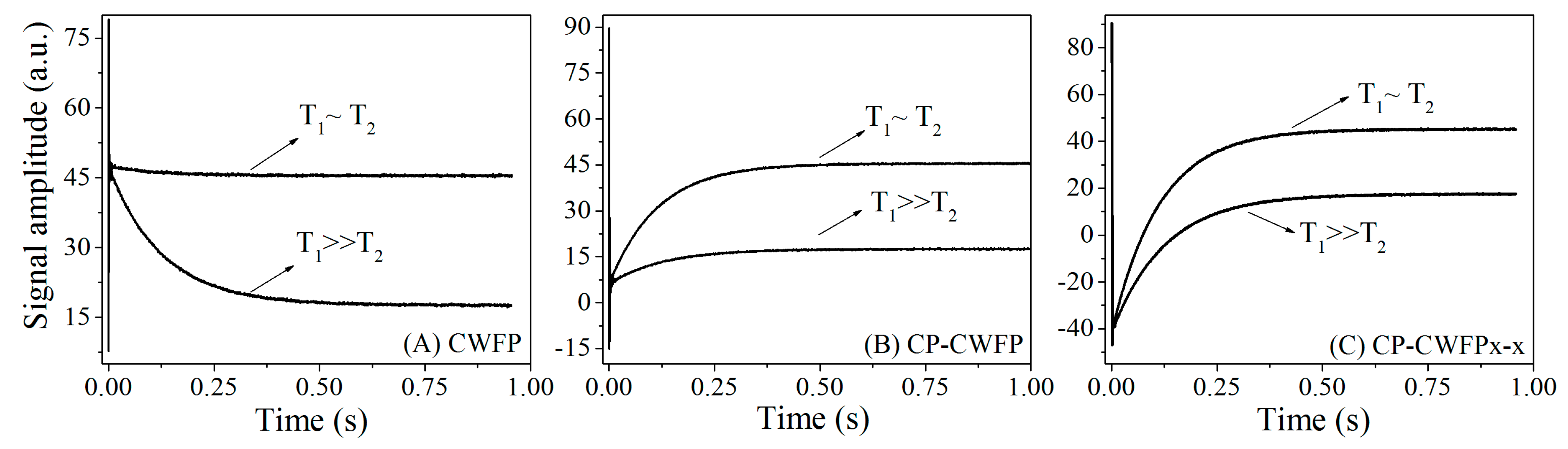
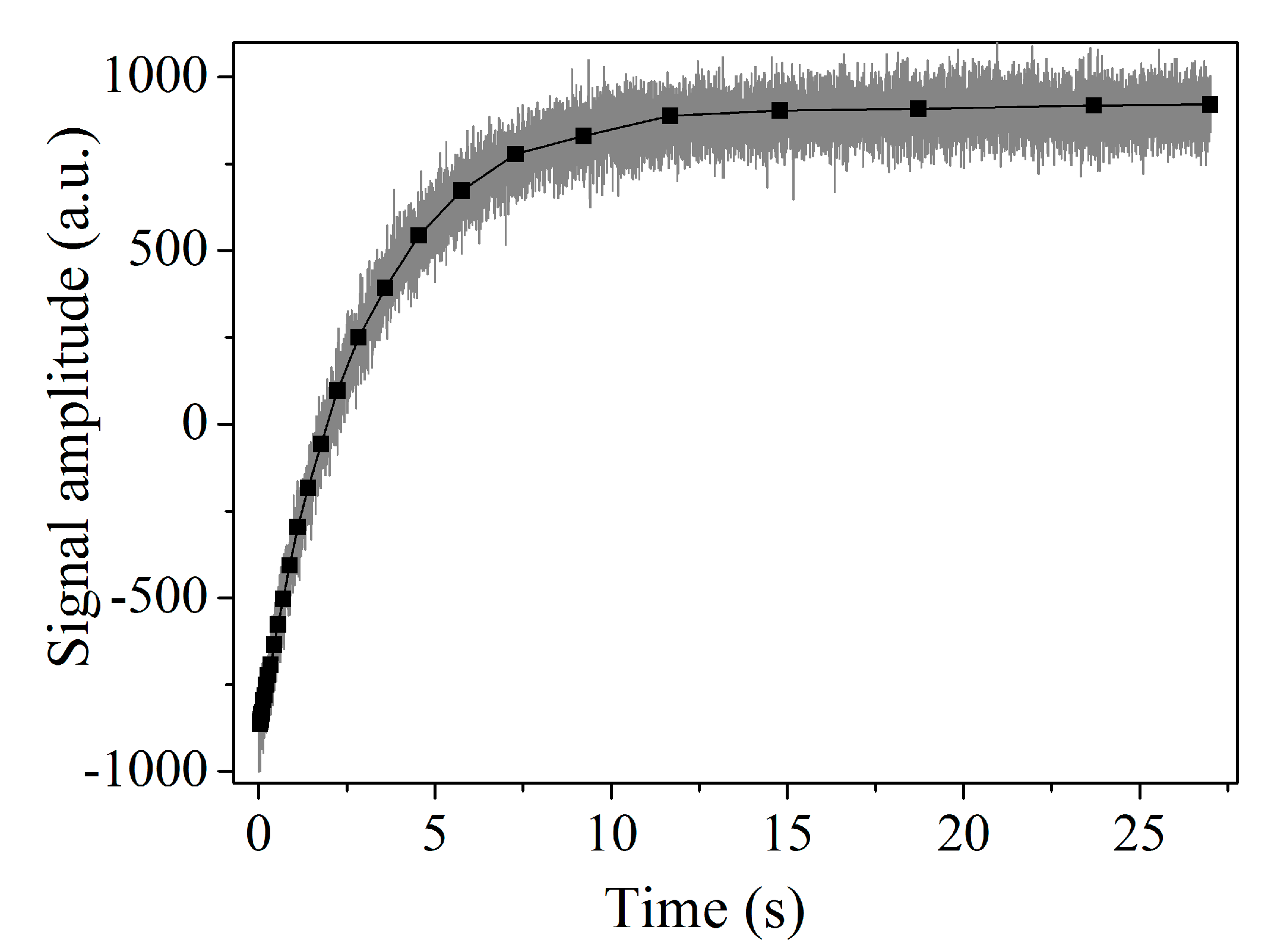
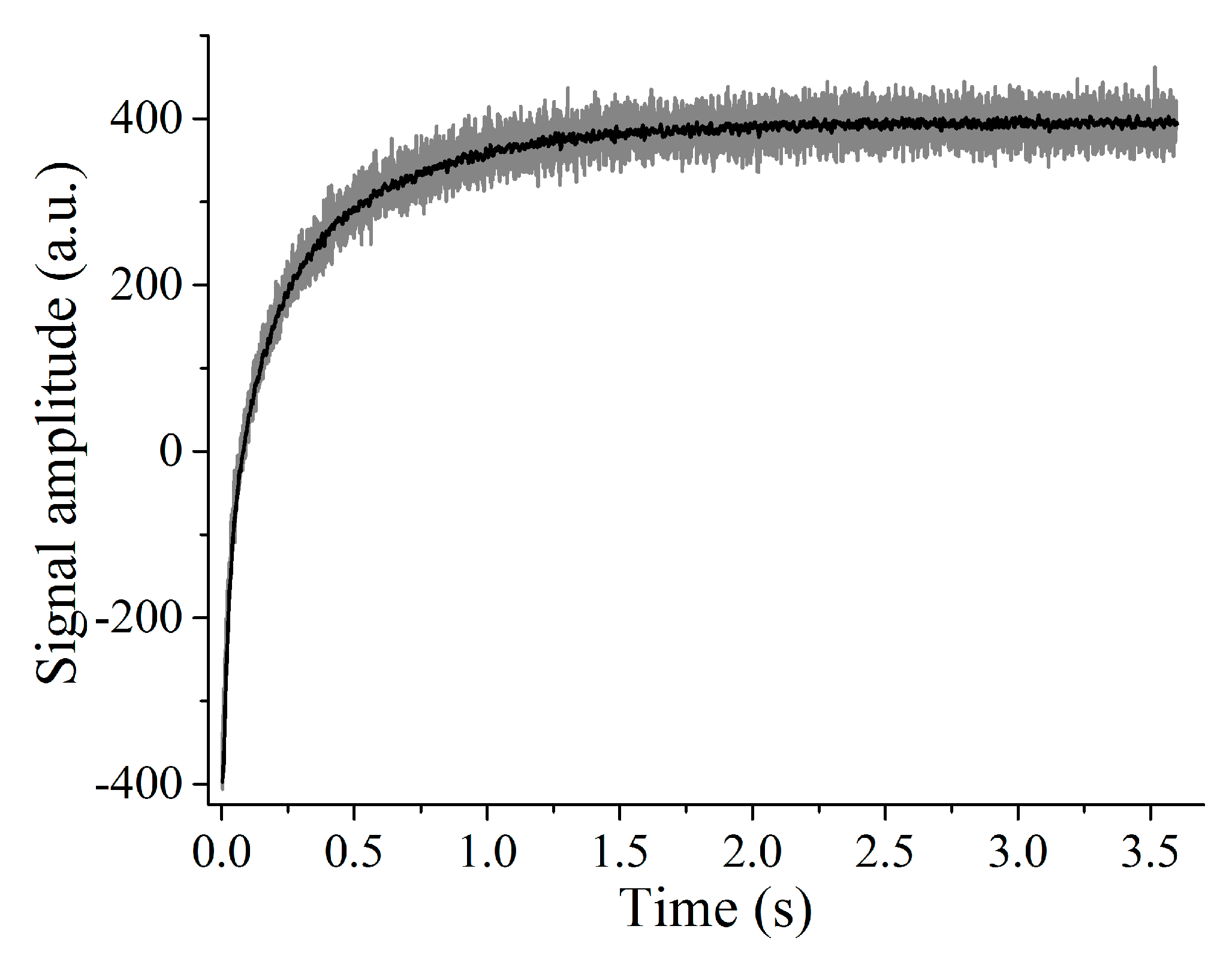
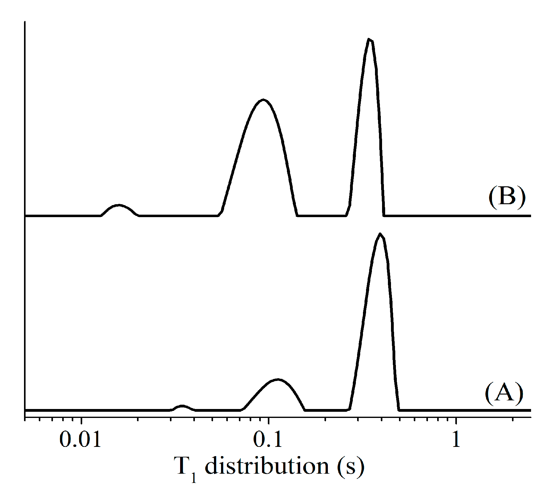
4.1. Fast and Simultaneous T₁ and T₂ Measurements

In 1977, Kronenbitter and Schwenk [30] proposed the use of the transient time T* (Equation (4)) of the SSFP signal to measure T₁ and T₂ using two experiments. In the first experiment, the T₁/T₂ ratio was determined by measuring the amplitude of the SSFP signals as a function of the flip angle θ. The second experiment involved measuring the transient time T* at the optimum flip angle, yielding the T₁ + T₂ value. These results were used for the determination of both relaxation times.

Exploring the same dependence on the CWFP regime, Venâncio et al. [9] demonstrated that it is not necessary to use these two experiments to measure T₁ and T₂ when θ = 90°. They proposed a fast method to measure both relaxation times in a single CWFP experiment using the evolution of the magnitude of the CWFP from the first pulse to the steady state (Figure 8A). In this figure, the initial part of the signal (dark grey region) is characterized by a strong oscillation of the amplitude following odd and even pulses [9]. The amplitude of this signal decays with T₂*. When the oscillation ends, the signal was named a quasi-stationary state (QSS) (transition between dark and light grays regions). From the QSS point, the signal decays slowly with a time constant T* (light grey region), given by Equation (5), to reach the constant steady state amplitude |M_ss| (white region). For a CP-CWFP signal, the first oscillating signal (Figure 8B, dark grey) decays to a minimum signal (QSS). From this point, the signal also increases with T* (light grey) and reaches a constant steady state amplitude |M_ss| (white region) [27].

For θ = 90° and $\mathrm{\Phi }=\left(2n+1\right)\pi$, the transient time T* for the CWFP and CP-CWFP sequences in Equation (4) is only dependent on the relaxation times according to Equation (5):

$$T^{*}=\frac{2T_1{T}_2}{T_1+T_2}$$

(5)

A simple rearrangement of Equations (3) and (5), results in:

$$\frac{T_1}{T_2}=\frac{M_0-\left|M_{ss}\right|}{\left|M_{ss}\right|}$$

(6)

or the proper relaxations times:

$$T_1=\frac{T^{*}/2}{\left|M_{ss}\right|/M_0}\mathrm{and}{T}_2=\frac{T^{*}/2}{1-\left|M_{ss}\right|/M_0}$$

(7)

Therefore, both relaxation times can be calculated in a single-scan CWFP or CP-CWFP experiment using the magnitude of M₀ (intensity after the first pulse), magnitude at steady state |M_ss|, and T*, using Equation (7). The T* value is obtained by exponential fitting of the T* decay (light grey region in Figure 8). The obtained relaxation time values are equivalent to those obtained by inversion recovery (T1) and CPMG (T2) pulse sequences [37,38]. The major source of error in CWFP and CP-CWFP experiments is the |M₀| value, which is strongly dependent on the spectrometer dead time. Normally, the dead time has to be shorter than 10 μs.

The difference between CWFP and CP-CWFP sequences is the dynamic range (DR) of the T* signal that depends on the T₁/T₂ ratio. Figure 9 provides a comparison of the CWFP (Figure 9A) and CP-CWFP (Figure 9B) transient regimes for samples with T₁ ≈ T₂ and T₁ >> T₂. The T₁ ≈ T₂ and T₁ >> T₂ signals were acquired using CuSO₄ (T₁ ≈ j T₂), and MnSO₄ solution (T₁ = 4T₂), in a 20 MHz spectrometer. The DR for CWFP is the greatest for T₁ >> T₂ and narrowest for T₁ = T₂ (Figure 9A). Conversely, the DR of the CP-CWFP signal is the largest for the sample with T₁ = T₂, and the narrowest for T₁ >> T₂ (Figure 9B).

The dependence of DR of T* as a function of the relaxation times ratio was solved using the CP-CWFP with phase alternation, CP-CWFPx-x [24]. Figure 9C shows the CP-CWFPx-x signal for the sample with T₁ ≈ T₂ and T₁ >> T₂. This figure shows that the T* dynamic range is independent of T₁/T₂ ratio. Furthermore, the CP-CWFPx-x pulse sequence can be performed on resonance and therefore is the best CWFP sequence for measuring both relaxation times in a single experiment.

We demonstrated that the CP-CWFPx-x sequence can be used to measure T₁ in a single shot experiment using a low flip angle (5° to 10°), even in a spectrometer with a long dead time [23]. Using these small flip angles, the T* is strongly dependent on T₁ (Equation (4)). Figure 10 provides a comparison between the CP-CWFPx-x with low flip angle (CWFP-T₁) transition time T* signal, obtained with a single shot experiment, and inversion-recovery (IR) data obtained with 32 experiments. Although the SNR of CWFP-T₁ is much lower than obtained with IR, the T₁ values were similar.

We demonstrated that several post-acquisition digital filters (low pass, linear and logarithm compression, Savitzky–Golay, and Wavelet filters) can be used to enhance SNR in CWFP-T₁ signals without significant deviation of the T₁ values [39]. Figure 11 shows a SNR enhancement of one order of magnitude on CWFP-T₁ signal using second-order, a 41-points window, and a Savistiky–Golay (SG) filter. Therefore, filtered CWFP-T₁ can be a fast T₁ method, providing an alternative to CPMG for low-field NMR relaxation measurements.

4.2. Analysis of Products Using Transient Cwfp Signals

4.2.1. Agri-Food Products

Transient CWFP/CP-CWFP signals have been used to analyze agriculture and food products as a useful alternative to CPMG. The first application of CWFP transient signals, using 90° pulses, was to measure the fat content in beef samples. The measurement was based on the |M_ss|/M₀ ratio and the univariate statistic that shows a better correlation (r = 0.9) than T₂ (r = −0.25) to beef fat intramuscular content [26]. The full transient signals of beef samples were also analyzed using multivariate (chemometric) analysis. The multivariate analyses of CWFP have been used to classify beef samples based on animal sex or breed [26,40], to predict water loss during beef cooking, and fat and moisture contents [41]. More recently, we showed that CWFP-T₁ can be a simple method to measure fat content in beef [39]. Figure 12 shows the relaxation profile of two beef samples with 20% and 62% fat contents. The peak between 300 and 400 ms was assigned to meat and fat, and the signal at 100 ms to fat only. Therefore, samples with higher fat contents show a large 100 ms peak. The ratio of the area of these two peaks has been used to measure fat content in beef with higher precision than standard CWFP sequences [39].

The CWFP signals have been used to study the oilseed quality in static and flowing modes. CWFP and CP-CWFP signals have been used to measure oil viscosity and fatty acid composition using multivariate statistics [42,43].

4.2.2. Polymers

Transient CWFP signals were used to simultaneously measure the T₁ and T₂ relaxation times during fast polymerization reaction (10 min) of commercial epoxy resin [44]. The advantage of CWFP to measure T₁ and T₂ over conventional methods is that both relaxation times can be measured in a single reaction. The standard T₁ and T₂ methods (inversion-recovery and CPMG) require the use of two separated reaction samples that are not ideal, as the two reactions did not have the exact same rates. Rodrigues et al. [28,29] applied CWFP sequences to real-time monitoring of the polymerization crosslinking reaction of acrylamide-based hydrogels. The CP-CWFP results showed high sensitivity and time resolution when monitoring important parameters of radical polymerization. Rodrigues et al. [29] used CP-CWFP to study the polymerization of acrylamide using a redox-pair initiator system. They observed that T₁ was more sensitive than T₂ when monitoring the reaction, confirming it is a good probe to monitor monomer conversion in real time in an automated non-destructive fashion.

Koch et al. used the CP-CWFPx-x sequence to study the coagulation of chitosan (CS) in aqueous solution as a function of pH using T₁ and T₂ values [45]. They observed that the relaxation profile was dependent on CS concentration. The main relaxation differences were observed for the sample with the highest CS concentration of 2.2 g/L. At this concentration, both T₁ and T₂ were sensitive to the coagulation process at pH between 6 and 7. However, T₁ increases with pH and T₂ shows a remarkable decrease. This relaxation results suggest that CS is forming a supramolecular structure (gel) that entraps the water in confined regions, reducing water mobility.

4.2.3. Paramagnetic Complexes

CWFP sequences have also been used in the study of paramagnetic ions complexes. T₁ and T₂ relaxation profiles were used to study Ethylenediamine tetraacetic acid-paramagnetic (Cu²⁺, Fe³⁺, and Mn²⁺) ion complexes as function of pH. Figure 13 shows the T₁ (stars) and T₂ (open circle) profiles of the EDTA-Cu²⁺ complex measured with CWFP and CP-CWFP sequences (Figure 13a), and with IR and CPMG (Figure 13b). These results show the similarity between the relaxation profiles measured by classical and CWFP methods. The dotted line in Figure 13a is the relaxation profile of T₁ ≈ T₂ for the Cu²⁺ solution without EDTA. This relaxation profile is completely different from complex relaxation profiles.

Figure 13a demonstrates that the relaxation profiles show similar variations in the absorbance measured in 730 nm. The relaxation profiles can also be measured in a colorless complex, such as EDTA-Mn²⁺, which is not detected by spectrophotometry [46]. Spectrophotometry is a standard method used to study this complex. The CP-CWFPx-x sequence has been used in the complexation of biopolymers chitosan (CS) with paramagnetic ions (Cu²⁺, Fe^3, and Mn²⁺) as a function of pH [46]. The results indicated that CS strongly interacts with these ions and the complex CS-ion can be easily removed from the solution by centrifugation.

5. Conclusions

Given these results, CWFP sequences are a fast, simple, efficient, and robust method to enhance SNR. CWFP can be used in static and flowing quantitative analyses, to measure T₁ and T₂ in single shot experiments, and to measure T₁ in a single shot sequence in spectrometers with long dead time. Therefore, CWFP sequences can be used to increase the applications of TD-NMR in academia and industry.

References

1. Carr, H.Y. Steady-State Free Precession in Nuclear Magnetic Resonance. Phys. Rev. 1958, 112, 1693–1701. [Google Scholar] [CrossRef]
2. Ernst, R.R.; Anderson, W.A. Application of Fourier Transform Spectroscopy to Magnetic Resonance. Rev. Sci. Instrum. 1966, 37, 93–102. [Google Scholar] [CrossRef]
3. Freeman, R.; Hill, H.D.W. Phase and intensity anomalies in fourier transform NMR. J. Magn. Reson. 1969 1971, 4, 366–383. [Google Scholar] [CrossRef]
4. Schwenk, A. NMR pulse technique with high sensitivity for slowly relaxing systems. J. Magn. Reson. 1969 1971, 5, 376–389. [Google Scholar] [CrossRef]
5. Dos Santos, P.M.; de Souza, A.A.; Colnago, L.A. Fast Acquisition of 13C NMR Spectra using the Steady-state Free Precession Sequence. Appl. Magn. Reson. 2011, 40, 331. [Google Scholar] [CrossRef]
6. Moraes, T.B.; Santos, P.M.; Magon, C.J.; Colnago, L.A. Suppression of spectral anomalies in SSFP-NMR signal by the Krylov Basis Diagonalization Method. J. Magn. Reson. 2014, 243, 74–80. [Google Scholar] [CrossRef] [PubMed] [Green Version]
7. Bangerter, N.K.; Hargreaves, B.A.; Vasanawala, S.S.; Pauly, J.M.; Gold, G.E.; Nishimura, D.G. Analysis of multiple-acquisition SSFP. Magn. Reson. Med. 2004, 51, 1038–1047. [Google Scholar] [CrossRef] [Green Version]
8. Miller, K.L. FMRI using balanced steady-state free precession (SSFP). NeuroImage 2012, 62, 713–719. [Google Scholar] [CrossRef] [Green Version]
9. Venâncio, T.; Engelsberg, M.; Azeredo, R.B.V.; Alem, N.E.R.; Colnago, L.A. Fast and simultaneous measurement of longitudinal and transverse NMR relaxation times in a single continuous wave free precession experiment. J. Magn. Reson. 2005, 173, 34–39. [Google Scholar] [CrossRef]
10. Freed, D.E.; Scheven, U.M.; Zielinski, L.J.; Sen, P.N.; Hürlimann, M.D. Steady-state free precession experiments and exact treatment of diffusion in a uniform gradient. J. Chem. Phys. 2001, 115, 4249–4258. [Google Scholar] [CrossRef]
11. Azeredo, R.B.d.V.; Engelsberg, M.; Colnago, L.A. Flow sensitivity and coherence in steady-state free spin precession. Phys. Rev. E 2001, 64, 016309. [Google Scholar] [CrossRef]
12. Bagueira de Vasconcelos Azeredo, R.; Colnago, L.A.; Engelsberg, M. Quantitative Analysis Using Steady-State Free Precession Nuclear Magnetic Resonance. Anal. Chem. 2000, 72, 2401–2405. [Google Scholar] [CrossRef]
13. Azeredo, R.B.V.; Colnago, L.A.; Souza, A.A.; Engelsberg, M. Continuous wave free precession: Practical analytical tool for low-resolution nuclear magnetic resonance measurements. Anal. Chim. Acta 2003, 478, 313–320. [Google Scholar] [CrossRef]
14. Hills, B.P. Applications of Low-Field NMR to Food Science. Annu. Rep. NMR Spectrosc. 2006, 58, 177–230. [Google Scholar] [CrossRef]
15. Marigheto, N.; Venturi, L.; Hills, B. Two-dimensional NMR relaxation studies of apple quality. Postharvest Biol. Technol. 2008, 48, 331–340. [Google Scholar] [CrossRef]
16. Van Duynhoven, J.; Voda, A.; Witek, M.; Van As, H.; Webb, G. Time-Domain NMR Applied to Food Products. Annu. Rep. NMR Spectrosc. 2010, 69, 145–197. [Google Scholar] [CrossRef]
17. Zalesskiy, S.S.; Danieli, E.; Blümich, B.; Ananikov, V.P. Miniaturization of NMR Systems: Desktop Spectrometers, Microcoil Spectroscopy, and “NMR on a Chip” for Chemistry, Biochemistry, and Industry. Chem. Rev. 2014, 114, 5641–5694. [Google Scholar] [CrossRef]
18. Maiwald, M.; Klas, M.; Zientek, N.; Kern, S. Process control with compact NMR. TrAC Trends Anal. Chem. 2016, 83, 39–52. [Google Scholar] [CrossRef]
19. Stueber, D.; Jehle, S. Quantitative Component Analysis of Solid Mixtures by Analyzing Time Domain 1H and 19F T1 Saturation Recovery Curves (qSRC). J. Pharm. Sci. 2017, 106, 1828–1838. [Google Scholar] [CrossRef]
20. Ge, X.; Chen, H.; Fan, Y.; Liu, J.; Cai, J.; Liu, J. An improved pulse sequence and inversion algorithm of T 2 spectrum. Comput. Phys. Commun. 2017, 212, 82–89. [Google Scholar] [CrossRef]
21. Kirtil, E.; Cikrikci, S.; McCarthy, M.J.; Oztop, M.H. Recent Advances in Time Domain NMR & MRI Sensors and Their Food Applications. Curr. Opin. Food Sci. 2017, 17, 9–15. [Google Scholar] [CrossRef]
22. Rondeau-Mouro, C. 2D TD-NMR Analysis of Complex Food Products. In Mordern Magnetic Resonance; Springer: Berlin, Germany, 2017; pp. 1–20. [Google Scholar] [CrossRef]
23. Moraes, T.B.; Monaretto, T.; Colnago, L.A. Rapid and simple determination of T1 relaxation times in time-domain NMR by Continuous Wave Free Precession sequence. J. Magn. Reson. 2016, 270, 1–6. [Google Scholar] [CrossRef]
24. Monaretto, T.; Andrade, F.D.; Moraes, T.B.; Souza, A.A.; deAzevedo, E.R.; Colnago, L.A. On resonance phase alternated CWFP sequences for rapid and simultaneous measurement of relaxation times. J. Magn. Reson. 2015, 259, 174–178. [Google Scholar] [CrossRef]
25. Carosio, M.G.A.; Fernandes, D.F.; Andrade, F.D.; Moraes, T.B.; Tosin, G.; Colnago, L.A. Measuring thermal properties of oilseeds using time domain nuclear magnetic resonance spectroscopy|Request PDF. J. Food Eng. 2015, 173, 143–149. [Google Scholar] [CrossRef]
26. Pereira, F.M.V.; Bertelli Pflanzer, S.; Gomig, T.; Lugnani Gomes, C.; de Felício, P.E.; Alberto Colnago, L. Fast determination of beef quality parameters with time-domain nuclear magnetic resonance spectroscopy and chemometrics. Talanta 2013, 108, 88–91. [Google Scholar] [CrossRef] [Green Version]
27. Andrade, F.D.d.; Marchi Netto, A.; Colnago, L.A. Use of Carr–Purcell pulse sequence with low refocusing flip angle to measure T1 and T2 in a single experiment. J. Magn. Reson. 2012, 214, 184–188. [Google Scholar] [CrossRef] [PubMed]
28. Rodrigues, E.J.R.; Sebastião, P.J.O.; Tavares, M.I.B. 1H time domain NMR real time monitoring of polyacrylamide hydrogels synthesis. Polym. Test. 2017, 60, 396–404. [Google Scholar] [CrossRef]
29. Rodrigues, E.J.d.R.; Neto, R.P.C.; Sebastião, P.J.O.; Tavares, M.I.B. Real-time monitoring by proton relaxometry of radical polymerization reactions of acrylamide in aqueous solution. Polym. Int. 2018, 67, 675–683. [Google Scholar] [CrossRef]
30. Kronenbitter, J.; Schwenk, A. A new technique for measuring the relaxation times T1 and T2 and the equilibrium magnetization M0 of slowly relaxing systems with weak NMR signals. J. Magn. Reson. 1969 1977, 25, 147–165. [Google Scholar] [CrossRef]
31. Webb, A. Increasing the Sensitivity of Magnetic Resonance Spectroscopy and Imaging. Anal. Chem. 2012, 84, 9–16. [Google Scholar] [CrossRef]
32. Colnago, L.A.; Engelsberg, M.; Souza, A.A.; Barbosa, L.L. High-Throughput, Non-Destructive Determination of Oil Content in Intact Seeds by Continuous Wave-Free Precession NMR. Anal. Chem. 2007, 79, 1271–1274. [Google Scholar] [CrossRef]
33. Pusiol, D. Apparatus and Method for Real Time and Real Flow-Rate Measurement of Multi-Phase Fluids. U.S. Patent 20060020403A1, 26 January 2006. [Google Scholar]
34. Colnago, L.A.; Azeredo, R.B.V.; Coelho, I.; Tavares, M.I.B.; Engelsberg, M. Analysis of the Photopolymerization Rate of Methacrylate Blends by Continuous Wave Free Precession NMR. Ann. Magn. Reson. 2003, 2, 125–127. [Google Scholar]
35. Venâncio, T.; Engelsberg, M.; Azeredo, R.B.V.; Colnago, L.A. Thermal diffusivity and nuclear spin relaxation: A continuous wave free precession NMR study. J. Magn. Reson. 2006, 181, 29–34. [Google Scholar] [CrossRef]
36. Duarte, C.J.; Colnago, L.A.; de Vasconcellos Azeredo, R.B.; Venâncio, T. Solvent Suppression in High-Resolution 1H NMR Spectroscopy Using Conventional and Phase Alternated Continuous Wave Free Precession. Appl. Magn. Reson. 2013, 44, 1265–1280. [Google Scholar] [CrossRef]
37. Meiboom, S.; Gill, D. Modified Spin-Echo Method for Measuring Nuclear Relaxation Times. Rev. Sci. Instrum. 1958, 29, 688–691. [Google Scholar] [CrossRef]
38. Kingsley, P.B. Methods of measuring spin-lattice (T1) relaxation times: An annotated bibliography. Concepts Magn. Reson. 1999, 11, 243–276. [Google Scholar] [CrossRef]
39. Monaretto, T.; Souza, A.; Moraes, T.B.; Bertucci-Neto, V.; Rondeau-Mouro, C.; Colnago, L.A. Enhancing signal-to-noise ratio and resolution in low-field NMR relaxation measurements using post-acquisition digital filters. Magn. Reson. Chem. 2018. [Google Scholar] [CrossRef]
40. Santos, P.M.; Corrêa, C.C.; Forato, L.A.; Tullio, R.R.; Cruz, G.M.; Colnago, L.A. A fast and non-destructive method to discriminate beef samples using TD-NMR. Food Control 2014, 38, 204–208. [Google Scholar] [CrossRef]
41. Corrêa, C.C.; Forato, L.A.; Colnago, L.A. High-throughput non-destructive nuclear magnetic resonance method to measure intramuscular fat content in beef. Anal. Bioanal. Chem. 2009, 393, 1357–1360. [Google Scholar] [CrossRef]
42. Constantino, A.F.; Lacerda, V., Jr.; Santos, R.B.d.; Greco, S.J.; Silva, R.C.; Neto, Á.; Barbosa, L.L.; Castro, E.V.R.d.; Freitas, J.C.C. Análise do teor e da qualidade dos lipídeos presentes em sementes de oleaginosas por rmn de baixo campo. Quím. Nova 2014, 37, 10–17. [Google Scholar] [CrossRef] [Green Version]
43. Colnago, L.A.; Azeredo, R.B.V.; Marchi Netto, A.; Andrade, F.D.; Venâncio, T. Rapid analyses of oil and fat content in agri-food products using continuous wave free precession time domain NMR. Magn. Reson. Chem. 2011, 49, S113–S120. [Google Scholar] [CrossRef]
44. Venâncio, T.; Colnago, L.A. Simultaneous measurements of T1 and T2 during fast polymerization reaction using continuous wave-free precession NMR method. Magn. Reson. Chem. 2012, 50, 534–538. [Google Scholar] [CrossRef]
45. Kock, F.V.C.; Colnago, L.A. Rapid method for monitoring chitosan coagulation using low-field NMR relaxometry. Carbohydr. Polym. 2016, 150, 1–4. [Google Scholar] [CrossRef]
46. Kock, F.V.C.; Colnago, L.A. Rapid and simultaneous relaxometric methods to study paramagnetic ion complexes in solution: An alternative to spectrophotometry. Microchem. J. 2015, 122, 144–148. [Google Scholar] [CrossRef]
Figure 1. Nuclear magnetic resonance (NMR) signals simulated numerically using θ = 90°, T1 = 200 ms, T2 = 150 ms, T2* = 0.5 ms and several Tp values. (A) Tp = 5T1, (B) Tp = T2, (C) Tp = 2T2*, in (D) and (E) Tp = 0.3 ms < T2*. The frequency offset is (AD) 5.0 kHz and (E) 3.3333 kHz. Grey bars indicate the position of the applied pulses.
Applsci 09 01312 g001
Figure 2. (A) Continuous Wave Free Precession (CWFP) and (B) Carr-Purcell Continuous Wave Free Precession (CP-CWFP) pulse sequences with phases (ϕ), flip angle (θ = θ1 = 90°) and time between pulses (Tp) shorter than the relaxation time T2* (Tp < T2*). (A) ϕ1 = ϕ2 is the original CWFP sequence without phase alternation and ϕ1 = −ϕ2 is the 180° phase alternation (CWFPx-x). (B) ϕ = ϕ1 = ϕ2 is the original CP-CWFP pulse sequence and (ϕ = ϕ1 = −ϕ2) is the 180° phase alternation CP-CWFPx-x. Adapted from Publication [24], Copyright (2015), with permission from Elsevier.
Applsci 09 01312 g002
Figure 3. Simulated magnitude profiles of CWFP signals. (A) CWFP and CP-CWFP profiles and (B) CWFPx-x and CP-CWFPx-x profiles. Solid lines represent the profiles for T p = 300 μs and dashed lines represented T p = 200 μs. Adapted from Publication [24], Copyright (2015), with permission from Elsevier.
Applsci 09 01312 g003
Figure 4. (A) Free induction decay (FID) and spin echo (SE) signals for a corn seed obtained in 15 s with a spin-echo sequence with τe = 3.5 ms, 16 scans. (B) CWFP signal for the same sample and the same acquisition time of 15 s (16,666 acquisition windows of 3Tp), using 90° pulses, Tp = 0.3 ms, and Φ = 5π. Adapted from Publication [13], Copyright (2003), with permission from Elsevier.
Applsci 09 01312 g004
Figure 5. (A) Magnitude of CWFP signal in arbitrary unit (au) as a function of oil concentration of the sunflower oil dissolved in carbon tetrachloride, r = 0.997. (B) Magnitude of CWFP signal as a function of hydrogen content in various solvents: (1) chloroform, (2) 1,1,1 trichloroethane, (3) 1,2 dichloroethane, (4) benzene, (5) cyclohexane, and (6) hexane; r = 0.998. Adapted from Publication [12], Copyright (2000), with permission from ACS Publications.
Applsci 09 01312 g005
Figure 6. (A) CWFP signal amplitude corresponding to 48 macadamia nut fragments with oil masses ranging from 0.1 to 0.7 g. (B) Oil mass as a function of CWFP peak amplitude for macadamia nut fragments with oil masses ranging from 0.1 to 0.7 g. A total of 96 peaks were obtained in a time of 14 s. The linear regression determination coefficient was R2 = 0.95. Adapted from Publication [32], Copyright (2007), with permission from ACS Publications.
Applsci 09 01312 g006
Figure 7. Amplitude of CWFP signal of the irradiated methacrylates samples with phenyl-propanedione (PPD, a), monoacylphosphine oxide (MAPO, b) and canphorquinone (c) photoinitiators.
Applsci 09 01312 g007
Figure 8. Numerically simulated signals showing the evolution of the (A) CWFP and (B) CP-CWFP signal magnitudes from the first pulse to the stationary state (|Mss|) using T1 = 150 ms, T2 = 50 ms, Tp = 0.3 ms, and T2* = 20 ms. When the oscillation ends, the signal was named a quasi-stationary state (QSS) (transition between dark and light grays regions). The background color indicates the first transient oscillating signal (dark grey), the slowly signal decay with time constant T* (light grey), given by Equation (5), until it reaches the constant steady state amplitude |Mss| (white region).
Applsci 09 01312 g008
Figure 9. Experimental (A) CWFP, (B) CP-CWFP, and (C) CP-CWFPx-x signal for solution of CuSO4 10 mM (T1 = T2) and MnSO4 1 mM solution (T1 >>T2).
Applsci 09 01312 g009
Figure 10. Comparison of Inversion recovery (IR) (black points) and Continuous Wave Free Precession- T 1 (CWFP- T 1 ) (grey line) normalized signals of water sample. Adapted from Publication [23], Copyright (2016), with permission from Elsevier.
Applsci 09 01312 g010
Figure 11. Original (gray) and denoised (black) continuous wave free precession (CWFP- T 1 ) signals using a second-order Savitzky–Golay filter with 41-data-point windows of a MnSO4 aqueous solution. The signal to noise ratio (SNR) of the original and smoothed data signals are 39 and 374, respectively.
Applsci 09 01312 g011
Figure 12. T1 distribution time of obtained by the inverse Laplace transform of a CWFP-T1 signal acquisition of beef samples with different fat contents: (A) 20% and (B) 62%. Adapted from Publication [39], Copyright (2014), with permission from Wiley.
Applsci 09 01312 g012
Figure 13. (a) Variation in maximum absorbance at 730 nm (■), T1 (☆) and T2 (○) measured simultaneously with CP-CWFP pulse sequence for the aqueous solution of complex Cu(II)- Ethylenediamine tetraacetic acid and T2 measured with CPMG (□) to the aqueous solution of Cu2+, in function of pH. In all experiments the Cu2+ concentration was 3.3 × 10⁻³ mol/L. The solid line for EDTA complexes is the sixth-order polynomial fitting of the data. The dashed line for Cu2+ solution is a sigmoidal fit. (a) Variation in T1 (☆) and T2 (○) of the same solution in (a), obtained with standard inversion-recovery (IR) and Carr–Purcell–Meiboom–Gill (CPMG) pulse sequences, respectively. Adapted from Publication [46], Copyright (2015), with permission from Elsevier.
Applsci 09 01312 g013