Bacterial Foraging-Based Algorithm for Optimizing the Power Generation of an Isolated Microgrid

Abstract

An Isolated Microgrid (IMG) is an electrical distribution network combined with modern information technologies aiming at reducing costs and pollution to the environment. In this article, we implement the Bacterial Foraging Optimization Algorithm (BFOA) to optimize an IMG model, which includes renewable energy sources, such as wind and solar, as well as a conventional generation unit based on diesel fuel. Two novel versions of the BFOA were implemented and tested: Two-Swim Modified BFOA (TS-MBFOA), and Normalized TS-MBFOA (NTS-MBFOA). In a first experiment, the TS-MBFOA parameters were calibrated through a set of 87 independent runs. In a second experiment, 30 independent runs of both TS-MBFOA and NTS-MBFOA were conducted to compare their performance on minimizing the IMG using the best parameter tuning. Results showed that TS-MBFOA obtained better numerical solutions compared to NTS-MBFOA and LSHADE-CV, an Evolutionary Algorithm, found in the literature. However, the best solution found by NTS-MBFOA is better from a mechatronic point of view because it favors the lifetime of the IMG, resulting in economic savings in the long term.

1. Introduction

Currently, one of the most critical issues is the efficient use of available energy sources. Therefore, in rural or remote geographic locations, the generation and distribution of energy is a significant challenge for many areas of engineering such as control, power electronics or planning, among others. In recent years, microgrids (MGs) have been a reliable solution for the power supply in separate areas, provided that there is adequate operational planning of the MG energy sources [1].

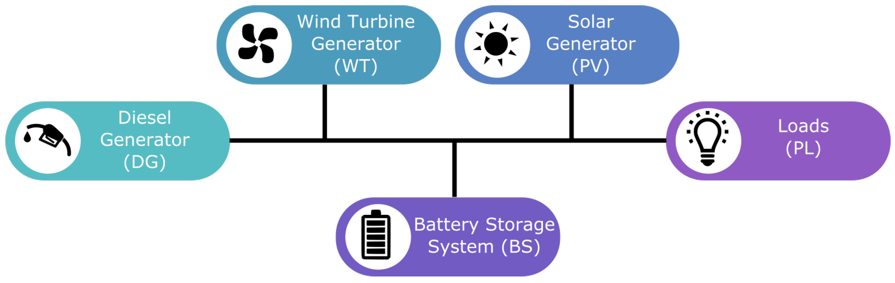
In general, an MG is composed of energy storage systems (ESS),hybrid power generation systems (HPGS) from renewable energy sources (RES) and conventional generation systems (CGS); with all elements working in a coordinated way for the power generation. It is important to highlight that CGSs have a high operating cost due to the materials and transportation logistics. Moreover, ESSs are integrated by costly devices requiring a safe manner operation, thus guaranteeing a long service life. Finally, uncertainty in the appropriate operation of the RES due to the origin of wind and sunlight must take into account. These theoretical considerations are some of the reasons why optimal management of power generation resources for the appropriate operation of the MG is required.

In isolated microgrids (IMGs), a hybrid power generation system (HPGS) is responsible for the generation of reliable energy. This is done by integrating into the IMG at least one of the RES, CGS, and ESS systems such as a wind turbine generator, solar generator, diesel generator, or battery storage systems. However, due to the RES generation intermittency, the ESS become the main factor in the steady performance of the IMGs [2,3,4]. When a steady state is reached, the best performance of the whole system is obtained. HPGSs have been studied by several authors [5,6,7], describing conditions of remote localities having variable demand and power dispatch by generators minimizing the cost of generation, while maintaining a balance between the generation of energy and the load.

Usually, the power supply to the load in an IMG can be calculated as an economic dispatch function for generators at a large-scale power level [8]. This cost function should be minimized, subject to constraints related to the generator’s capacity and the energy balance between generation and load demand. The load demand must be computed for a 24 h period in an IMG, and several scenarios can be presented in the HPGS such as: (1) RESs cannot produce energy for 24 h; (2) all the RES in the IMG can always dispatch energy, but not the total demand capacity of the load; (3) the main costs are the fuel costs and the generation of the diesel generator; and (4) the operation cost of the HPGSs are non-linear, generally due to the cost of the diesel generator.

On the other hand, there is a kind of problems, specifically in real-world applications, where it is impossible to find an optimal solution using a viable amount of resources employing traditional techniques such as numerical methods or graphic analysis. These cases correspond to the hard optimization category and have a similar nature to the NP (nondeterministic polynomial time) decision problems since they can not be solved in an optimal way or up to a guaranteed point using deterministic methods in polynomial time.

Metaheuristics are an alternative to find feasible and optimal solutions to NP problems, where any problem modeled as a constrained numerical optimization problem (CNOP) can have at least one optimal feasible solution. A CNOP also known as a general problem of non-linear programming can be defined as: minimize $f\left(\overrightarrow{x}\right)$ subject to: $g_i\left(\overrightarrow{x}\right)\le 0$, $i=1,\cdots ,m$ or $h_j\left(\overrightarrow{x}\right)=0$, $j=1,\cdots ,p$. Here, $\overrightarrow{x}\in {\mathbb{R}}^n$ such that $n\ge 1$, is the solution vector $\overrightarrow{x}={[x_1,x_2,\cdots ,x_n]}^T$, where each $x_i$, $i=1,\cdots ,n$ is delimited by the lower and upper limit $L_i\le x_i\le U_i$; m is the number of inequality constraints and p is the number of equality constraints (in both cases, the constraints can be linear or non-linear). If we denote by F the feasible region (where all the solutions that satisfy the problem are found) and by S the entire search space, then $F\subseteq S$.

Metaheuristics are well-known algorithms, most of them are inspired by nature, that have successfully solved CNOPs. Metaheuristics are divided into two broad groups: (1) evolutionary algorithms (EAs), whose operation is based on emulating the process of natural evolution and survival of the fittest [9], and (2) swarm intelligence algorithms (SIAs) that base their operation on social and cooperative behaviors of simple organisms such as insects, birds, and bacteria [10].

From the initial ideas of Bremermann [11], in 2002 Passino proposed a novel SIA called Bacterial Foraging Optimization Algorithm (BFOA) [12], based on E.Coli bacteria foraging. In BFOA, each bacterium E. Coli tries to maximize the energy obtained per unit of time spent on the foraging process, while avoiding harmful substances. Moreover, bacteria can communicate with each other by segregating certain substances. There are four main processes in BFOA: (1) chemotaxis (swim-tumble movements), (2) swarming (communication between bacteria), (3) reproduction (cloning of the best bacteria), and (4) elimination-dispersal (replacement of the worst bacteria). Bacteria are potential solutions to the problem and their location represents the values of the problem decision variables. Bacteria can move (generate new solutions) through the chemotaxis cycle; additionally, a movement through the attraction of solutions in promising areas of the search space is generated (as it allows the reproduction of the best solutions). Finally, those bacteria located in areas of low quality are deleted.

In 2009, a simplified BFOA version was proposed, called modified bacterial foraging optimization algorithm (MBFOA) [13], which implements fewer parameters with respect to the original BFOA. MBFOA includes a mechanism for the management of constraints based on feasibility rules, consisting of (a) between two feasible solutions, that with the best value in the objective function is selected, (b) between a feasible solution and a non-feasible solution, the feasible one is selected, and (c) between two non-feasible solutions, the one with the smallest amount of constraint violations is selected [14]. MBFOA has been used to solve a number of problems of a different nature. For example, solving a set of chemical and mechanical engineering design problems, obtaining competitive results [13], and the solution of a bi-objective mechanical design problem with constraints [15].

In 2016, a recent algorithm based on MBFOA, called two-swim MBFOA (TS-MBFOA) [16], was proposed. This version includes an operation similar to the mutation operator, used in EAs, as a swimming operator within the chemotaxis process. It also implements a random swim in the chemotaxis process, along with a skew mechanism for the initial population based on the variables range. TS-MBFOA has been used to solve real-world problems of mechatronic design and also in the nutrition field by generating successful healthy menus [17].

There is a number of proposals in the specialized literature using metaheuristics algorithms to optimize particular mathematical models minimizing or maximizing an MG. Some of the EAs employed are Differential Evolution and Genetic Algorithms. SIAs employed are limited to particle swarm optimization (PSO) and BFOA. Other paradigms such as artificial neural networks, harmony search, and hybridizations between harmony search and differential evolution have also been used [18,19,20]. A common factor in this works is the management of constraints using the penalty technique, which implies adding more parameters to be defined by the end user.

In

Table 1. Algorithms used for smartgrid optimization.

Author	Algorithm	Type of Electrical Distribution Network	Objective	Experimental Scenario
Hernández-Ocaña et al.	TS-MBFOA/NTS-MBFOA	Isolated Micro grid (IMG)	Operation cost, balance between energy generation and its demand by the load	Home area
Ahmad et al. (2018) [21]	BFOA/Tabu Search	Smart Grid	Waiting time and electricity cost	Single home with different Operational time Interval
Hasan et al. (2018) [22]	BFOA/Strawberry Algorithm	Smart Grid	Electricity cost and Peak to Average Ratio	Home Energy Management System (Single home)
Saadia et al. (2018) [23]	BFOA	Smart Grid/Pigeon Inspired Optimization	Electricity cost and Peak to Average Ratio	Home Energy Management System (Single home)
Wang et al. (2015) [24]	Genetic Algorithm	Smart Micro-Grid	Operation cost	The building micro-grid system with distributed generation, energy storage device, electric vehicle and various load resources
Ma et al. (2015) [25]	PSO	Islanded Micro-Grid	Overall generating cost	Islanded microgrid with renewable energy source, the diesel generator and battery storage system
Wang et al. (2015) [26]	Game theory	Smart Grid	Efficiency in the power system and energy loss	The model was simulated and analyzed in modified IEEE 37-bus feeder system with DGs connected
Zhu et al. (2018) [27]	PSO	Battery Energy Storage	Optimization of both the placement and controller parameters for Battery Energy Storage Systems to improve power system oscillation damping	New England 39-bus system and a Nordic test system

, main proposals based on BFOA were grouped according to particular characteristics. Moreover, other proposals were added—each proposal derived in several contributions. In the first row, representing this work, BFOA is implemented in order to optimize a mathematical model minimizing an IMG, including renewable energy sources such as wind and solar, as well as a conventional generation unit based on diesel fuel. Two novel versions of the BFOA are implemented and tested: TS-MBFOA, and a new proposal called NTS-MBFOA. Results showed that TS-MBFOA obtained better numerical solutions compared to NTS-MBFOA and compared to LSHADE-CV, an EA found in the literature solving the same problem. However, the best solution found by NTS-MBFOA is better from a mechatronic point of view because it favors the lifetime of the IMG and therefore resulting in economic savings in the long term.

In the second row of Table 1, Ahmad and others [21] proposed the bacterial foraging tabu search (BFTS) technique, a hybridization of BFOA and tabu search (TS) using different operational time interval (OTI) to schedule appliances while balancing user comfort (UC). His goal was to reduce both the waiting time and electricity cost simultaneously. Real-time pricing (RTP) scheme was used to get the total cost of electricity consumed. For simulations, they studied an average size modern home with 11 appliances. The simulation results of BFTS-based scheduled clearly shows that the proposed technique is better as compared to BFOA, TS, and unscheduled electricity consumption. The electricity cost and waiting time were minimized thus increasing UC.

In the third row of Table 1, Hasan and others [22] implemented two algorithms aimed at minimizing electricity cost and peak to average ratio (PAR) in a smartgrid by using BFOA and strawberry algorithm (SBA). Real-time pricing (RTP) pricing scheme was used to calculate the electricity cost. A single home with three types of appliances; fixed, shiftable and elastic appliances composed the simulated model. Authors found that these optimization schemes reduce the total electricity cost and peak to the average ratio by shifting the load from on-peak hours to off-peak hours. BFOA performed better than SBA regarding electricity cost minimization. However, the authors concluded that trade-off always exists between cost and user comfort.

In the fourth row of Table 1, Saadia and others [23] gained electricity cost reduction up to 40% in a home energy management system (HEMS) with a single home using BFOA and pigeon inspired optimization (PIO). Cost, PAR and waiting time of the appliances were calculated on the bases of a 120 h time slot. Two types of appliances were used: interruptible and non-interruptible. Critical peak pricing (CPP) was used as a pricing signal to calculate the electricity bills. Simulation results showed that PIO was identified as the best technique as it performs well in reducing cost. PIO gives 37% more waiting time than BFOA; it has 60% less cost by BFOA and PAR is 3% less by BFOA.

In the fifth row of Table 1, Wang and others [24] implemented a genetic algorithm to optimize a micro-grid operation considering distributed generation, environmental factors and demand response (DR). Experiments were conducted on a smart micro-grid from Tianjin, China. The building micro-grid system mainly includes distributed generation, energy storage device, electric vehicle, and various load resources. Two prices mechanisms were used, fixed price and DR prices. The main finding of this model is to optimize the cost in the context of considering demand response and system operation without reducing user comfort. Also, the authors found that the natural gas price dramatically influences both the operation cost of the micro-grid and demand response.

In the sixth row of Table 1, Ma and others [25] focus on minimizing the overall system generating cost, including the depreciation cost, the operation cost, the pollutant emission cost, and economic subsidies available for renewable energy source (RES) over the entire dispatch period of an IMG. For experimentation, they use an actual IMG in Dongao Island, China. Authors applied a modified PSO algorithm to solve this optimization problem. Results showed that this algorithm was able to minimize both the fuel consumption cost and pollution emission cost.

In the seventh row of Table 1, Wang and others [26] proposed a distributed locational marginal pricing (DLMP)-based unified energy management system (uEMS) model, which considers both increasing profit benefits for distribution generations (DGs) and increasing stability of the distributed power system (DPS). The model contains two parts: (1) a game theory-based loss reduction allocation (LRA); and (2) a load feedback control (LFC) with price elasticity. Simulation results based on a modified IEEE 37-bus system show that uEMS can lead to a more fairly competitive environment for DGs, where the model can increase DGs’ benefits, reduce system losses, and improve stability.

In the last row of Table 1, Zhu and others [27] aimed to find the optimal placement and control parameter settings of multiple battery energy storage System (BESS) units to improve oscillation damping in a power transmission system. They formulated a mixed-integer optimization problem and solved it using PSO. Experiments were conducted on two power systems, the New England 39-bus system, and a Nordic test system. This optimization design can be adapted to seasonal load changes and the minimum number of BESS units to be placed. The superiority of the proposed model was validated with another typical type of controllers in the existing literature.

On the other hand, Aziz and others [28] investigated the techno-economic and environmental performance of a hybrid energy system (HES) under the load following (LF) and cycle charging (CC) strategies using HOMER software as a tool for optimization analysis. Experiments were conducted in a photovoltaic (PV)–diesel–battery configuration. Results show that variations in critical parameters, such as battery minimum state of charge, time step, solar radiation, diesel price, and load growth have considerable effects on the performance of the proposed system.

In summary, the problem of optimal management of energy sources in an IMG can be solved as a dispatch control problem, which deals with the energy flow management from the various sources to load for cost minimization.

This document is organized as follows: Section 2 presents the mathematical modeling of the Isolated Microgrid proposed. Section 3 and Section 4 briefly describe TS-MBFOA and the normalized version called NTS-MBFOA. In Section 5, results obtained and the discussion of these are presented. Finally, in Section 6, the conclusions and future works are presented.

2. Description of the Isolated MicroGrid

An IMG is composed of a set of AC loads and an HPGS. In this work, the HPGS is integrated by a solar photovoltaic generator (PV), a wind turbine generator (WT), a diesel generator (DG) and a battery storage system (BS), as shown in Figure 1.

The aim of the optimal management of energy sources in an IMG is to assign the load demands among its distributed generation units securely and reliably, to minimize the overall system generating cost, subject to a set of constraints. Thus, it is essential to compute the operation cost of each of such generation units. In this work, the cost function and data for the BS, PV and WT generators were taken from [29] (2014 prices). In that work, the authors computed the corresponding cost function of the BS, PV, and WT considering the rate of return of the initial investment using a factor of capital recovery in a regular series of equal annual payments. Figure 2 depicts the overall optimization process proposed.

2.1. DG Generation Cost

The mathematical relationship associated with this kind of systems is related to the generator power. Without loss of generality, we established the cost function as:

$$F_i\left(P_i\right)={\alpha }_i+{\beta }_i{P}_i+{\gamma }_i{P}_i^2$$

(1)

where $F_i$ and $P_i$ are the i-th generation source and its output power, respectively. Also, $\alpha$, $\beta$ and $\gamma$ are the cost coefficients. Therefore, in this work the cost function for the DG systems is given by:

$$F_1\left(P_1\right)=1488+0.3P_1+0.000435P_1^2$$

(2)

2.2. BS Generation Cost

The general cost function, proposed in [29], is given by:

$$F\left(P\right)=a{I}^{p}P+G^{E}P$$

(3)

where P is the generator output power, a is the rate of return of the initial investment, $I^p$ is the inversion cost per installed unit and $G^E$ is the operation and maintenance costs per unit of generated power.

Also, the rate of return of the initial investment is computed by:

$$a=\frac{r}{1-{(1+r)}^{-N}}$$

(4)

where r the interest rate (we set a value of $0.09$ for the base case) and N the useful life (we propose 20 years), respectively.

In this work, we set a 2 kWh battery storage bank as the ESS system of the IMG. Therefore, the inversion cost per storage unit installed is established as $[I^p=1000$$/kW]. Also, the operation and maintenance costs per unit is given by $[G^E=$¢1.6/kW]. Finally, the cost function is given by:

$$F_2\left(P_2\right)=119P_2$$

(5)

2.3. PV Generation Cost

The PV generation cost was computed using a inversion cost per installed unit of $[I^p=5000$$/kW] and the operation and maintenance costs per unit given by $[G^E=$¢1.6/kW]. Therefore, the PV generation cost is computed by:

$$F_3\left(P_3\right)=545.016P_3$$

(6)

2.4. WT Generation Cost

To compute the cost function of the WT generator we use an inversion cost per installed unit given by $[I^p=5000$$/kW], and an operation and maintenance costs per unit given by $[G^E=$¢1.6/kW]. Thus, the cost function is computed by:

$$F_4\left(P_4\right)=152.616P_4$$

(7)

2.5. Optimization Strategy

In order to obtain an optimal power generation in an IMG, an economic dispatch problem must be solved. In this problem, the output power of each one of the IMG’s sources must be computed at every hour of the day, so that the generation cost is the lowest possible. In this study, the vector of design variables is related to the sources, therefore:

$$\overrightarrow{p}=\left[P_1,P_2,P_3,P_4\right]$$

(8)

where $P_i$ with $i=1,\cdots ,4$ is the output power of the i-th generation source.

2.6. Objective Function

The classical economic dispatch problem is established with:

$$minF=\sum _{i=1}^n{F}_i\left(P_i\right)$$

(9)

subject to the following constraints:

$$\begin{array}{c}\hfill \sum _{i=1}^n{P}_i=P_L\end{array}$$

(10)

$$\begin{array}{c}\hfill P_i^{min}\le P_i\le P_i^{max}\end{array}$$

(11)

where n is the number of generation sources, $P_i^{min}$ and $P_i^{max}$ are the minimum and maximum values of the output power of the i-th generation source, $P_L$ is the total load demanded by the system, and $F_i$ is the generation cost of the i-th generation source.

In this work, the objective function at $\tau$-hour is given by:

$$\begin{array}{c}\hfill F(\overrightarrow{p^{\tau }})={\omega }_1{C}_f{F}_1\left(P_1\left(\tau \right)\right)+{\omega }_2{F}_2\left(P_2\left(\tau \right)\right)\\ \hfill -{\omega }_3{F}_3\left(P_3\left(\tau \right)\right)-{\omega }_4{F}_4\left(P_4\left(\tau \right)\right)\end{array}$$

(12)

where ${\omega }_1$, ${\omega }_2$, ${\omega }_3$ and ${\omega }_4$ are the weights related with each one of the sources generation. These weights were fixed to $0.25$ while the fuel cost was set to USD $\$1$.

Finally, considering that the generation cost must be computed at every hour of the day, the total objective function for all the day is:

$$\mathrm{\Phi }=\sum _{\tau =1}^{24}F\left(\overrightarrow{p}\left(\tau \right)\right)$$

(13)

2.7. Design Constraints

In order to produce a proper management of the power generation in the IMG, we considered some design constraints.

• Power Balance: The sum of the generation power of all sources must be equal to the total load demanded by the system:

  $$P_1+P_2+P_3+P_4=P_L$$

  (14)
• BS Model: The output power of the solar PV generator and the load demanded at time t by the system, determine the state of charge (SOC) of the battery storage system BS. On the other hand, the SOC of the BS system at hour t, SOC(t), is related to the previous hour SOC, SOC($t-1$) [6]:

  $$SOC\left(t\right)=SOC(t-1)-{\alpha }_D{P}_2\left(t\right)+{\alpha }_C{P}_3\left(t\right)+{\alpha }_C{P}_4\left(t\right)$$

  (15)

  where ${\alpha }_D={\eta }_D/B_C^{max}$ and ${\alpha }_C={\eta }_C/B_C^{max}$, in which ${\eta }_D$ and ${\eta }_D$ are the battery charging efficiency and the battery discharging efficiency, respectively. Also, $B_C^{max}$ is the maximum battery capacity.
  Using Equation (15), a general mathematical equation by the battery dynamics can be established as:

  $$\begin{array}{c}\hfill SOC\left(t\right)=SOC\left(0\right)-{\alpha }_D\sum _{\tau =1}^t{P}_2\left(\tau \right)+{\alpha }_C\sum _{\tau =1}^t{P}_3\left(\tau \right)\\ \hfill +{\alpha }_C\sum _{\tau =1}^t{P}_4\left(\tau \right)\end{array}$$

  (16)

  where $SOC\left(0\right)$ is the initial state of charge of the battery, ${\alpha }_C{\sum }_{\tau =1}^t{P}_3\left(\tau \right)+{\alpha }_C{\sum }_{\tau =1}^t{P}_4\left(\tau \right)$ is the input power by the battery and ${\alpha }_D{\sum }_{\tau =1}^t{P}_2\left(\tau \right)$ is the power discharged by the battery at time t, respectively.
  Finally, at time t the state of charge of the battery must be between the minimum ($SO{C}^{min}$) and maximum ($SO{C}^{max}$) possible capacity:

  $$SO{C}^{min}\le SOC\left(t\right)\le SO{C}^{max}$$

  (17)

In this work, the BS parameters are shown in

Table 2. Energy Storage System parameters.

ESS Parameter	%
Round Trip efficiency	85
Charge efficiency	85
Discharge efficiency	100
Maximum state of charge	95
Minimum state of charge	40

.

2.8. Optimization Problem

We defined the mono-objective optimization problem associated with the optimal power generation as:

$$min\mathrm{\Phi }=\sum _{\tau =1}^{24}F\left(\overrightarrow{p}\left(\tau \right)\right)\overrightarrow{p}\left(\tau \right)\in {\mathbb{R}}^4$$

(18)

subject to the constraints:

$$\begin{array}{ccc}\hfill h_1\left(\overrightarrow{p}\left(\tau \right)\right)& =& P_1\left(\tau \right)+P_2\left(\tau \right)+P_3\left(\tau \right)+P_4\left(\tau \right)=P_L\hfill \\ \hfill g_1\left(\overrightarrow{p}\left(\tau \right)\right)& =& SO{C}^{min}-SOC\left(\tau \right)\le 0\hfill \\ \hfill g_2\left(\overrightarrow{p}\left(\tau \right)\right)& =& SOC\left(\tau \right)-SO{C}^{max}\le 0\hfill \end{array}$$

(19)

with the bounds:

$$\begin{array}{ccc}\hfill 0& \le & P_1\left(\tau \right)\le D{G}_{nominal}\hfill \\ \hfill 0& \le & P_2\left(\tau \right)\le SOC\left(0\right)\times B_{cmax}-SO{C}^{min}\times B_{cmx}\hfill \\ \hfill 0& \le & P_3\left(\tau \right)\le P_{pv}\left(\tau \right)\hfill \\ \hfill 0& \le & P_4\left(\tau \right)\le P_{wind}\left(\tau \right)\hfill \end{array}$$

(20)

where $D{G}_{nominal}$ is the nominal capacity of the DG system and $B_{cmax}$ is the maximum capacity of the battery system; with proposed values of 5000 kW and 2000 kW, respectively. Values of $P_{pv}$ and $P_{wind}$ were taken from [30]. Indeed, values of $P_{pv}\left(\tau \right)$ and $P_{wind}\left(\tau \right)$ (where $P_{pv}$ is the photovoltaic output power and $P_{wind}$ is the wind output power) are based on studies conducted on real data. For the photovoltaic resource, two-day solar irradiation data collected in Celestún (México) was used. For the wind resource, data collected in Celestún (México), Ambewela (Sri Lanka), and Madrid (Spain) for several heights was used. In this study, these ranks are used as input values for the TS-MBFOA and NTS-MBFOA at each run to find the minimum value optimizing the IMG.

Table 3. Starting conditions (in Watts and percentages) of the resources included in the IMG. $L_P$ = Load power, $P_1$ = Diesel power, $P_2$ = ESS, $P_3$ = Solar power and $P_4$ = Wind power.

Time	${\mathit{L}}_{\mathit{P}}$	${\mathit{P}}_{\mathbf{1}}$	${\mathit{P}}_{\mathbf{2}}$	${\mathit{P}}_{\mathbf{3}}$	${\mathit{P}}_{\mathbf{4}}$
	Watts	Watts	%	Watts	Watts
00:00	2500	5000	0.950	1	1
01:00	2500	5000	0.949	1	500
02:00	2850	5000	0.737	1	750
03:00	2950	5000	0.630	1	600
04:00	2850	5000	0.482	1	1000
05:00	2500	5000	0.629	1	700
06:00	2150	5000	0.653	1	350
07:00	2250	5000	0.480	266	1
08:00	2300	5000	0.480	70	1
09:00	2320	5000	0.480	560	1
10:00	2350	5000	0.551	700	1
11:00	2950	5000	0.656	126	600
12:00	2250	5000	0.585	840	1700
13:00	2320	5000	0.950	840	2500
14:00	2350	5000	0.950	700	3000
15:00	2350	5000	0.950	560	5000
16:00	2450	5000	0.950	406	7000
17:00	3150	5000	0.950	63	7000
18:00	3310	5000	0.950	1	4000
19:00	4250	5000	0.950	1	1000
20:00	4250	5000	0.525	1	500
21:00	3000	5000	0.525	1	550
22:00	2950	5000	0.592	1	6500
23:00	2650	5000	0.950	1	5700

summarizes the initial power in Watts (W) and percentages (for the ESS) of each resource in the IMG per hour.

3. Two-Swim Modified Bacterial Foraging Optimization Algorithm (TS- MBFOA)

TS-MBFOA is an algorithm derived from MBFOA proposed to solve CNOPs [16]. In this metaheuristic, a bacterium i represents a potential solution to the CNOP (i.e., a n-dimensional real-value vector identified as $\overrightarrow{x}$), and it is defined as ${\theta }^i(j,G)$, into a population of bacteria ($S_b$), where j is the chemotaxis loop ($N_c$). G is the generational loop that ends up reaching a maximum number of generations ($GMAX$) or using a number of evaluations, defined by the user, calculated as:

$$GMAX=\frac{\mathit{Number}\mathit{of}\mathit{evaluations}}{S_b\times N_c}.$$

(21)

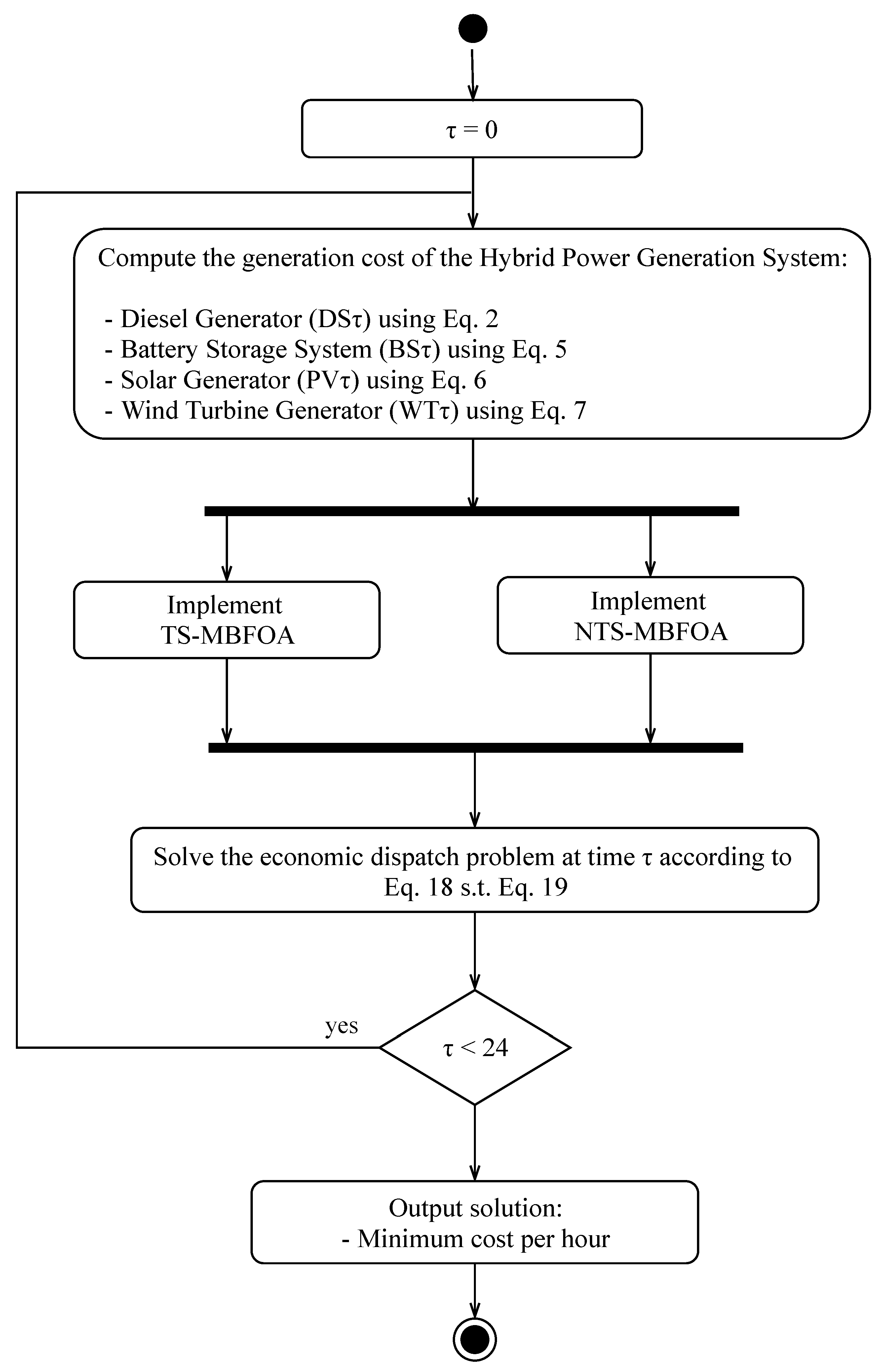
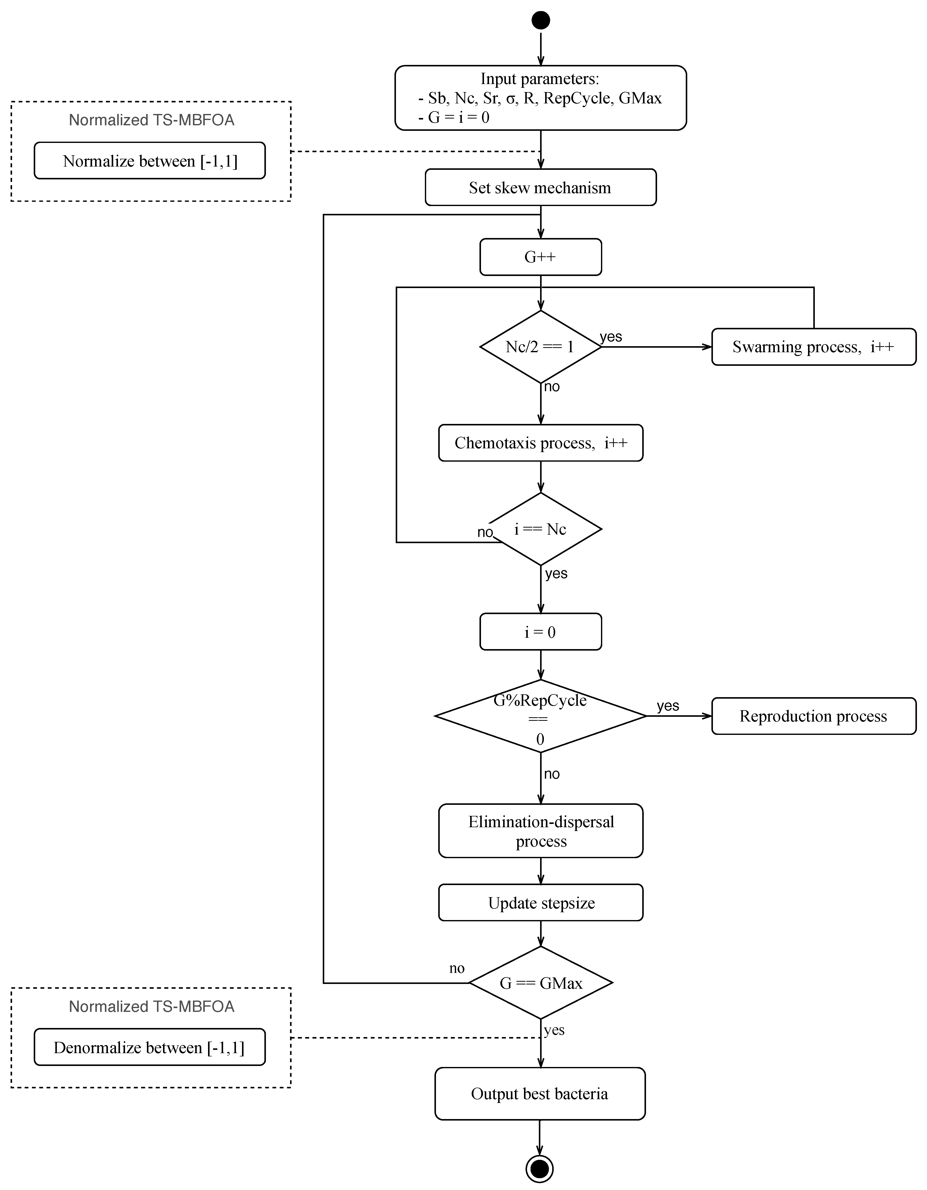
A generation includes the following processes: (1) a chemotaxis process with $N_c$ loops; (2) a swarming towards the best bacterium of the swarm ${\theta }^B\left(G\right)$; (3) a reproduction process, if the frequency parameter $RepCycle$ (defined by the user) allows it, with the best bacteria of the swarm $S_r$; and finally (4) an elimination-dispersal process that eliminates the worst bacterium of the swarm.

Chemotaxis: In this process, two swims are interleaved in each generation: either the exploitation swim or exploration swim is performed. The process starts with the exploitation swim (classical swim). Yet, a bacterium will not necessarily interleave exploration and exploitation swims, because if the new position of a given swim ${\theta }^i(j+1,G)$ has better fitness (based on the feasibility rules) than the original position ${\theta }^i(j,G)$, another swim at the same direction will take place in the next loop. Otherwise, a new tumble is computed. The process stops after $N_c$ attempts.

The exploration swim uses the mutation between bacteria and is calculated by:

$${\theta }^i(j+1,G)={\theta }^i(j,G)+\left(\sigma \right)({\theta }_1^r(j,G)-{\theta }_2^r(j,G))$$

(22)

where ${\theta }_1^r(j,G)$ and ${\theta }_2^r(j,G)$ are two different randomly selected bacteria from the population. Additionally, $\sigma$ is a parameter defined by the user used in the swarming operator, which defines the proximity of the new position of a bacterium with respect to the position of the best bacteria in the population ${\theta }^B\left(G\right)$. In this operator, $\sigma$ is a positive control parameter for scaling the different vectors in (0,1), i.e., scales of the area where a bacterium can move.

The exploitation swim is calculated as:

$${\theta }^i(j+1,G)={\theta }^i(j,G)+C(i,G)\varphi \left(i\right)$$

(23)

where $\varphi \left(i\right)$ is calculated with the original tumble operator of BFOA:

$$\varphi \left(i\right)=\frac{\Delta \left(i\right)}{\sqrt{\Delta {\left(i\right)}^T\Delta \left(i\right)}}$$

(24)

where $\Delta {\left(i\right)}^T$ is a random vector with elements within the range $[-1,1]$.

$C(i,G)$ is the random step size of each bacterium updated by:

$$C(i,G)=R*\mathrm{\Theta }\left(i\right)$$

(25)

where $\mathrm{\Theta }\left(i\right)$ is a randomly generated vector of size n with elements within the range of each decision variable: $[U_x,L_x]$, $x=1,\cdots ,n$, and R is a user-defined parameter for scaling the step size (this value must be close to zero, for example 5.00E-04). The initial $C(i,0)$ is generated using $\theta \left(i\right)$. This random step size allows bacteria to move in different directions within the search space and prevents premature convergence, as suggested in [31]. Step size R can be randomly, statically, and dynamically adjusted [32].

Swarming: At the half number of the chemotaxis process, the swarming operator is applied with (where $\sigma$ is a user-defined positive parameter between (0,1)):

$${\theta }^i(j+1,G)={\theta }^i(j,G)+\sigma ({\theta }^B\left(G\right)-{\theta }^i(j,G))$$

(26)

where ${\theta }^i(j+1,G)$ is the new position of the bacterium i, ${\theta }^B\left(G\right)$ is the current position of the best generational bacterium and $\sigma$, is a parameter called scaling factor, which regulates how close the bacterium i will be from the best bacterium ${\theta }^B$. In this proposal, if a solution violates the boundary of decision variables then a new solution of $x_i$ is randomly generated between the lower and upper limits $L_i\le x_i\le U_i$ of the decision variables. The swarming operator movement applies twice in a chemotaxis loop, while in the remaining steps the tumble-swim movement is carried out.

Reproduction: In this process, bacteria are ordered based on the handling constraint technique, duplicating the best bacteria $S_r$, and eliminating the same number of worst bacteria to maintain the size of the population. The process is carried out once every certain number of cycles which is a user-defined parameter $1\le RepCycle\le GMAX$, it aims to allow the diversity in the swarm.

Elimination-dispersal: Finally, the worst bacterium of the population ${\theta }^w(j,G)$ is eliminated based on the feasibility rules, and a new one is randomly generated.

The original proposal of TS-MBFOA includes a skew mechanism to generate the random initial population and a local search engine. However, in this study we did not include this mechanism in order to reduce computational cost. The pseudocode of TS-MBFOA is presented in Algorithm 1.

Algorithm 1: TS-MBFOA pseudocode. $S_b$ is the number of bacteria, $N_c$ is the number of chemotaxis cycles, $\sigma$ is the scaling factor, R is the stepsize, $S_r$ is the number of bacteria to reproduce, $Repcycle$ is the reproduction frequency and $GMAX$ is the number of generations.

4. Normalized Two-Swim Modified Bacterial Foraging Optimization Algorithm (NTS-MBFOA)

Normalization is the operation in which a set of values of a certain magnitude are transformed into another one, on a predetermined scale. In this work, normalization represents a change of magnitude at a fixed scale to map the search space of the TS-MBFOA to a range of $[-1,1]$, and so obtain a better performance of the algorithm solving the IMG problem [33]. We employ the following to normalize the bacterial population, as proposed in [34]:

$${\theta }_x^i(j,0)=\frac{{\theta }_x^i(j,0)}{U_x},x=1,\cdots ,n$$

(27)

where $x^i$ is a decision variable, ${\theta }_x^i(j,0)$ is the value to normalize the bacterium’s current position, and $U_x$ is the upper limit of the variable $x_i$.

Denormalization of results consists of the inverse operation, which is a simple multiplication as is defined in:

$${\theta }_x^i(j,G)={\theta }_x^i(j,G)\times U_x,x=1,\cdots ,n$$

(28)

The pseudocode of NTS-MBFOA is presented in Algorithm 2. The new bacterium generated in the elimination-dispersal process is also normalized using Equation (27). The best and worst bacterium are selected according to the feasibility rules of Deb [14], using the objective function value and the sum of violated constraints. In this algorithm, bacteria are ordered from best to worst. First, bacteria are denormalized and evaluated both in the objective function and the problem constraints. Subsequently, bacteria are ordered. The set of ordered bacteria is again normalized to continue with the following algorithm processes. Figure 3 describes the TS-MBFOA operation.

Algorithm 2: NTS-MBFOA pseudocode. $S_b$ is the number of bacteria, $N_c$ is the number of chemotaxis cycles, $\sigma$ is the scaling factor, R is the step size, $S_r$ is the number of bacteria to reproduce, $Repcycle$ is the reproduction frequency and $GMAX$ is the number of generations.

5. Results

We implemented TS-BFOA and NTS-MBFOA to solve the IMG problem on three computers with the following characteristics: a PC with 4 GB RAM, 2.3 Ghz processor; and two PCs with 8.0 GB RAM, 2.4 GHz processor. We use the Matlab R2018b development platform over a 64 bit Windows operating system.

5.1. First Experiment

First, we calibrate the parameters for TSM-BFOA and NTS-MBFOA via 87 independent runs with a diverse combination of parameters and 15,000 generations. The ranges tested for each parameter were: $S_b$ between [10, 200], $N_c$ between [5,100], $S_r$ between [1, $S_b/2$], $RepCycle$ between [10, 200], $R,B$ between [0,1] and $GMAX$ between [5000,15,000]. The best result obtained from all the independent runs was the value −564,959.112. During the calibration phase, we noticed that the higher the number of bacteria and chemotaxis cycles, the execution time of both algorithms increased from an order of seconds to minutes, due to the number of evaluations needed (number of times that a solution is evaluated in the objective function and constraints), which is calculated by $S_b\times N_c\times GMAX$. TS-MBFOA takes ∼14 min, on average, using the best combination of parameters. In the case of NTS-MBFOA, the algorithm takes ∼16 min on average. This time can be improved using a computer with a better processor.

We found that, by increasing the reproduction frequency ($RepCycle$) to values greater than 60, the results quality of the algorithm decreased, that is, the population of bacteria loses diversity. Therefore, a lower number of bacteria $S_r$ favors the performance of the algorithm.

Finally, values close to zero for the step size R and scaling factor B allow a better balance between exploitation and exploration of the search space and have a positive impact on the performance of the algorithm when generating higher quality solutions according to the objective function.

From these experiments, the best parameter calibration is presented in

Table 4. Parameters of TS-MBFOA and NTS-MBFOA.

Parameter	TS-MBFOA/NTS-MBFOA
$S_b$	10
$N_c$	8
$S_r$	5
R	$0.015$
$\sigma$	$0.040$
$RepCycle$	60
$GMAX$	15,000

.

5.2. Second Experiment

We ran independently both TS-MBFOA and NTS-MBFOA 30 times with the parameter configuration obtained in the previous experiment. The statistical results of both algorithms are shown in

Table 5. Basic Statistics of the results obtained by TS-MBFOA and NTS-MBFOA compared against an Evolutionary Algorithm. Std is the standard deviation.

Statistic	LSHADE-CV	TS-MBFOA	NTS-MBFOA
Best	−5.33E+05	−5.52E+05	−5.49E+05
Median	−5.32E+05	−4.98E+05	−4.92E+05
Average	−5.32E+05	−4.81E+05	−4.89E+05
Worst	−5.32E+05	−3.45E+05	−3.78E+05
Std.	8.73E+01	4.86E+04	4.40E+04
Evaluations	2.88E+05	1.20E+06	1.20E+06

. The standard deviation is calculated using the best solution found in each of the 30 independent runs, where the best solution is the sum of the 24 objective functions in a run.

TS-MBFOA obtained the best solution with a value of −551,960.121 followed by NTS-MBFOA with a value −549,369.785 in the objective function. Values are negative because they represent an economic saving when operating with RES, instead of using only the diesel generator and the ESS (battery). The more energy supplied by the RES and the less supplied by the DG and the ESS, the higher the savings.

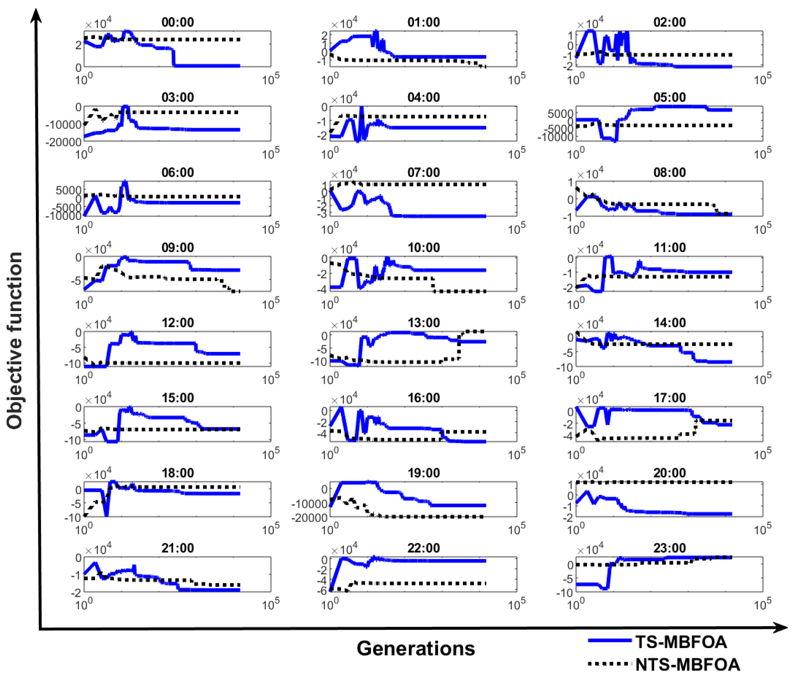
A convergence graph was generated for TS-MBFOA and NTS-MBFOA using the data of the independent run number 15 (representing the median). In Figure 4, we can observe the behavior of each algorithm during the 24 h, both algorithms starting with infeasible solutions. For the NTS-MBFOA, feasible solutions arise in the first ∼10 generations, except for hours 16:00, 17:00, and 23:00, where the algorithm requires more generations. For the TS-MBFOA, solutions are found beyond 200 generations. As can be observed in Figure 4, the NTS-MBFOA converges more quickly on feasible solutions, which indicates a lower computational cost than TS-BFOA.

With respect to the quality of the solutions found by the algorithms in each of the 24 h, the convergence graphs indicate that both algorithms behave differently along the day, but in hours 00:00, 02:00–04:00, 06:00–07:00, 13:00–14:00, 16:00–18:00 and 22:00–23:00 the TS-MBFOA algorithm generates better feasible solutions. In the rest of the hours, NTS-MBFOA generates a better solution to the objective function. In run number 15, the TS-MBFOA obtained a value of −525,869.49 in the objective function, in the case of NTS-MBFOA the value found was −422,989.41.

Results of bacterial foraging-based algorithms are better when compared against the LSHADE-CV algorithm. However, a higher number of evaluations is required. Parameters reported by the authors of LSHADE-CV algorithm are presented in

Table 6. Parameters of LSHADE-CV. D is the number of decision variables of the problem, in this case D = 4.

Parameter	LSHADE-CV
NP (Population)	90 (dynamic)
Generations	334
PCV	0.1
H	6
$N^{init}$	D × $r^{N^{init}}$
$N^{min}$	4
$r^{N^{init}}$	18

. LSHADE-CV dynamically tuned the parameters using operators such as parameter memory and linear population reduction [35]. The best numeric solution was −532,508.057. Besides, BFOAs obtained a better median, average, standard deviation and the worst value found is close to the average.

Analyzing the results of the TS-MBFOA and the NTS-MBFOA, we observed that NTS-MBFOA has a lower standard deviation than the TS-MBFOA because it finds the better among the worst results, that is, results closer to the average. To know if there is a significant difference between the NTS-MBFOA and TS-MBFOA algorithms, we conducted the non-parametric Wilcoxon Signed Rank Test, with a confidence level of 95% to the set of the 30 best solutions obtained of the 30 independent runs of each algorithm. The result obtained by this test was a p value of 0.00112, which implies that there is a significant difference between the results of both algorithms.

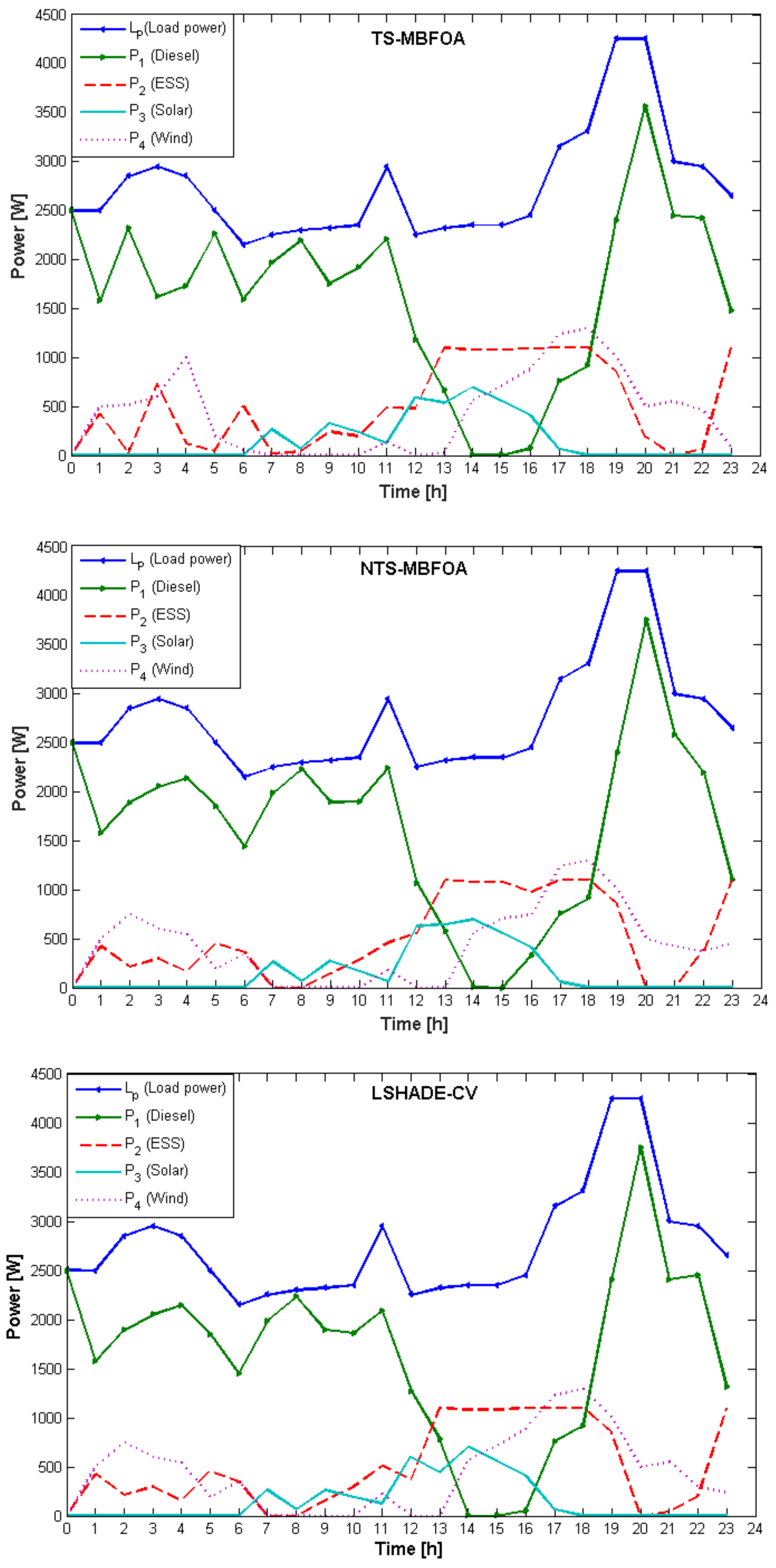
To analyze results from the mechatronic point of view, we used the values of the best solution generated by TS-MBFOA, NTS-MBFOA, and LSHADE-CV, respectively, for the IMG during the 24 h. Values presented in

Table 7. Details of the best solution found by the TS-MBFOA.

Time	$P1$ (Diesel)	$P2$ (ESS)	$P3$ (Solar)	$P4$ (Wind)	Load	Objective F.
00:00	2496.3651	1.6701	1	0.9649	2500	745.2825
01:00	1575.6793	423.8042	0.5166	500	2500	−6147.3127
02:00	2318.9864	15.5409	1	514.4727	2850	−18,540.63612
03:00	1620.3690	729.4394	0.1916	600	2950	−806.8983
04:00	1726.7810	122.2190	1	1000	2850	−34,196.74276
05:00	2260.0548	44.1808	0.9957	194.7687	2500	−5523.7952
06:00	1592.7925	505.2331	0.5558	51.4187	2150	13,392.21051
07:00	1962.2575	20.7425	266	1	2250	−35,095.00219
08:00	2190.8451	38.9401	70	0.2148	2300	−7697.4964
09:00	1752.4745	240.1307	327.14	0.2548	2320	−36,970.82458
10:00	1916.7460	195.5353	237.5564	0.1623	2350	−26,010.00763
11:00	2203.3221	487.8177	126	132.8602	2950	−7027.6669
12:00	1179.4551	480.6729	589.8720	7.61E-05	2250	−65,828.93738
13:00	665.9984	1094.7179	535.9387	23.3450	2320	−41,244.7373
14:00	0.0081	1079.7260	700	570.2659	2350	−85,010.15548
15:00	0.0038	1079.7280	560	710.2682	2350	−71,276.1857
16:00	71.2158	1092.9549	405.9995	879.8298	2450	−56,363.05636
17:00	755.8825	1099.9999	63	1231.1175	3150	−22,708.51646
18:00	915.8824	1100	0.9084	1293.2093	3310	−16,576.23946
19:00	2399.4340	850.26	0.3059	1000	4250	−12,090.66619
20:00	3562.3782	187.5911	0.0307	500	4250	−11,849.35186
21:00	2449	2.67E-14	1	550	3000	−20,281.31989
22:00	2422.4054	63.8122	0.1824	463.6	2950	−14,991.08009
23:00	1474.9268	1100	0.7396	74.3335	2650	30,139.01468

,

Table 8. Details of the best solution found by the NTS-MBFOA.

Time	$\mathit{P}\mathbf{1}$ (Diesel)	$\mathit{P}\mathbf{2}$ (ESS)	$\mathit{P}\mathbf{3}$ (Solar)	$\mathit{P}\mathbf{4}$ (Wind)	Load	Objective F.
00:00	2497.9398	0.9465	1	0.1135	2500	757.2053
01:00	1573.9146	425.4661	0.6192	500	2500	−6112.5895
02:00	1887.5926	212.4112	1	748.9960	2850	−21,861.4483
03:00	2050.6453	298.9427	0.4118	600	2950	−13,440.1448
04:00	2139.6755	165.0924	0.6572	544.5747	2850	−15,293.68
05:00	1850.0542	455.7456	1	193.2001	2500	6565.5218
06:00	1440.1282	362.7909	0.0617	347.0190	2150	−2118.2733
07:00	1983	9.74E-15	266	1	2250	−35,701.6365
08:00	2229	3.86E-12	70	1	2300	−8864.7210
09:00	1894.1196	147.9505	276.9766	0.9530	2320	−32,838.0707
10:00	1899.1742	280.8999	169.2419	0.6838	2350	−14,190.8007
11:00	2244.2556	458.7640	65.01756	181.9627	2950	−1433.49856
12:00	1069.9749	553.1234	626.9016	2.09E-11	2250	−68,753.9706
13:00	570.1086	1099.4087	645.9181	4.5644	2320	−55,393.8553
14:00	0.0040	1079.7278	700	570.2681	2350	−85,010.1842
15:00	1.18E-13	1079.7297	560	710.2702	2350	−71,276.2124
16:00	327.6886	975.1160	406	741.1953	2450	−54,549.0147
17:00	755.8823	1100	57.2461	1236.8715	3150	−22,144.0646
18:00	915.8823	1100	0.3844	1293.7331	3310	−16,524.8488
19:00	2399.9492	850.0232	0.0274	1000	4250	−12,059.4515
20:00	3749	5.47E-14	1	500	4250	−17,399.8776
21:00	2581.0778	0.5378	0.9855	417.3987	3000	−15,121.9325
22:00	2191.6068	383.0271	0.8398	374.5261	2950	−2318.6164
23:00	1099.3798	1100	0.3595	450.2606	2650	15,714.3807

and

Table 9. Details of the best solution found by LSHADE-CV.

Time	$\mathit{P}\mathbf{1}$ (Diesel)	$\mathit{P}\mathbf{2}$ (ESS)	$\mathit{P}\mathbf{3}$ (Solar)	$\mathit{P}\mathbf{4}$ (Wind)	Load	Objective F.
00:00	2496.2999	1.7	1	1	2500	744.7866
01:00	1573.6435	425.3572	0.9999	499.9992	2500	−6167.8006
02:00	1887.2143	211.7856	1	750	2850	−21,918.5478
03:00	2049.9383	299.063	0.9999	599.9985	2950	−13,517.0085
04:00	2145.3657	162.0959	0.9999	541.5383	2850	−15,310.5979
05:00	1850.8365	458.4619	1	189.7014826	2500	6780.1853
06:00	1448.8134	350.1865	1	350	2150	−2731.4501
07:00	1982.9999	1.59E-15	266	1	2250	−35,701.6365
08:00	2228.9999	3.15E-17	70	1	2300	−8864.721
09:00	1897.5368	160.1119	262.3511	2.56E-14	2320	−30,445.4635
10:00	1862.9841	298.6488	188.367	6.16E-17	2350	−16,260.0739
11:00	2086.0154	512.6329	126	225.351533	2950	−9881.8426
12:00	1272.2539	374.6484	603.0976	6.02E-14	2250	−70,753.5073
13:00	779.237	1100	440.7629	5.38E-14	2320	−27,202.5115
14:00	2.86E-12	1080	700	570.2702	2350	−85,010.2124
15:00	5.63E-13	1080	560	710.2702	2350	−71,276.2124
16:00	55.8823	1100	406	888.1176	2450	−56,471.1139
17:00	755.8823	1100	62.9915	1231.126	3150	−22,707.6927
18:00	915.8823	1100	1	1293.1176	3310	−16,585.2296
19:00	2398.1499	850.85	1	1000	4250	−12,168.4505
20:00	3748.9999	4.11E-16	1	500	4250	−17,399.8776
21:00	2405.6499	43.35	1	550	3000	−19,017.7949
22:00	2451.0823	205.8	1	292.1176	2950	−4318.2607
23:00	1307.8823	1100	1	241.1176	2650	23,676.9774

were used to generate the IMG behavior graphs shown in Figure 5, respectively. In these graphs, each resource is marked with different lines. In the case of the BFOAs, it is important to highlight that the conditions established for the use of solar and wind energy favor the high demand for diesel consumption (see Table 3).

Analyzing the behavior graphs of the TS-MBFOA and the NTS-MBFOA, we can observe that both algorithms produce similar results, i.e., both allow the consumption of solar and wind energy while decreasing the use of the diesel generator and the intervention of the battery (ESS).

Specifically, the use of solar power increases from 07:00 h onwards and decreases after 17:00 h, when the sun begins to hide. Concerning the wind power, both graphs show variations of peaks in the first hours, reaching a maximum production of energy close to 1250 watts between the 13:00 and 19:00 h. The ESS operates in a considerable and constant way between 13:00 h and 18:00 h. However, in the early hours of the day, the solution generated by TS-MBFOA presents several peaks (state transitions of the battery operation) that fall and rise abruptly, which decreases the battery’s lifetime.

The behavior of the solar and wind power, as well as ESS, tends to reduce the diesel demand from 12:00 h. Moreover, diesel is even not used for one hour, between 14:00 and 15:00 h, in both algorithms. However, when solar power is depleted, diesel power begins to rapidly increase. Analyzing the behavior of the use of diesel in the early hours of the day, it is evident that the NTS-MBFOA solution allows less diesel generator starts by having fewer peaks during the first hours of the day, which increases the lifetime of the diesel generator.

TS-MBFOA obtained a better solution in numbers, with $-551960.121$ in the objective function value, compared to NTS-MBFOA, that obtained a value of $-549,369.785$ in the objective function. The behavior of the graph lines, which correspond to the resources used in the IMG, favors the NTS-MBFOA because this solution increases the useful lifetime of the ESS and the DG, allowing economic savings on the long term.

Comparing the behavior graphs of the NTS-MBFOA and LSHADE-CV, we observe similar behavior in all the components of the IMG. Only from the hour 15:00 to 16:00 h it is evident how the EA delays the start of the diesel generator. On the other hand, from the hour 21:00 to 22:00 h, this algorithm starts the diesel generator slightly, something that does not happen in NTS-MBFOA. Since the graphs are very similar, we can take the numerical values as a point of comparison, where the best results of both algorithms were −549,369.785 and 532,508.057, respectively. We can conclude that both algorithms are competitive, but NTS-MBFOA obtains better results. However, the competitiveness of the evolutionary algorithm is evident, even with fewer generations than our proposal.

6. Conclusions

Two algorithms, TS-MBFOA and NTS-MBFOA, based on the foraging of the E. Coli bacteria were implemented to solve a CNOP minimizing an isolated microGrid (IMG). An IMG is an intelligent energy network that uses distributed generators allowing the exploitation of renewable energy sources, such as wind and solar, as well as fuels (e.g., diesel, petrol). The CNOP is based on a mathematical model, wherein the optimum values of a network of power generation devices are computed to supply a load during 24 h. In essence, every hour an optimization problem is solved, according to the conditions and operation restrictions of the network. As a result, we generate behavior graphs of the optimal powers, i.e., the sum of the 24 objective functions, which represents the best solution.

Two experiments were designed to monitor the behavior of the algorithms while minimizing the IMG. In the first experiment, 87 independent runs were conducted with different values to the parameters of the TS-MBFOA algorithm in order to obtain the best configuration of parameters that allows the optimal performance of the algorithm. As a result of this experiment, we obtained that the best performance of the algorithm was using a population of 10 bacteria, eight chemotaxis cycles, five bacteria to reproduce every 60 generations with a step size of 0.015 and a scaling factor of 0.040. We also noticed that, the higher the number of bacteria and chemotaxis cycles, the longer the execution time required by the algorithm.

In the second experiment, 30 independent runs of both TS-MBFOA and NTS-MBFOA were conducted, using the parameter tuning obtained in the previous experiment. The best solution obtained by TS-MBFOA was −551,960.121 and by NTS-MBFOA was −549,369.785, where a lower value is better, meaning economic savings. Both results are the sum of the 24 objective functions.

A non-parametric Wilcoxon signed rank test was conducted for the 30 best solutions of each of the algorithms, resulting in a significant difference between both algorithms.

Results obtained by TS-MBFOA and NTS-MBFOA were compared against the LSHADE-CV algorithm, where the best solution found by our proposals were better, although at a higher computational cost.

According to results, TS-MBFOA found a better numerical solution to the problem. From the mechatronic point of view, however, it is important to notice that NTS-MBFOA obtained a better result because it favors the useful life both of the diesel generator and the energy storage system (battery). This conclusion arises from a behavior analysis of each resource used by the IMG during the 24 h of a day.

As future work, more experiments will be conducted on TS-MBFOA and NTS-MBFOA to reduce the number of evaluations and find highly competitive solutions against other state-of-the-art algorithms. We are motivated in advance in the study of IMG for a real implementation in a low-consumption energy housing.

References

1. Bordons, C.; Torres, F.G.; Valverde, L. Gestión óptima de la energía en microrredes con generación renovable. Rev. Iberoam. Autom. Inf. Ind. RIAI 2015, 2, 117–132. [Google Scholar] [CrossRef]
2. Ross, M.; Hidalgo, R.; Abbey, C.; Joós, G. Energy storage system scheduling for an isolated microgrid. Renew. Power Gener. IET 2011, 5, 117–123. [Google Scholar] [CrossRef]
3. Carrasco, J.; Franquelo, L.; Bialasiewicz, J. Power electronic systems for the grid integration of renewable energy sources: A survey. IEEE Trans. Ind. Electron. 2006, 53, 1002–1016. [Google Scholar] [CrossRef]
4. Li, W.; Joos, G. Economic Dispatch Optimization of Microgrid Islanded Mode. In Proceedings of the IEEE Power Electronics Specialists Conference, Orlando, FL, USA, 17–21 June 2007; pp. 1280–1285. [Google Scholar]
5. Musseline, M.; Notton, G.; Louche, A. Design of hybrid-photovoltaic power generator with optimization of energy management. Sol. Energy 2005, 79, 33–46. [Google Scholar]
6. Tazvinga, H.; Xia, X.; Zhang, J. Minimum cost solution of photovoltaic-diesel-battery hybrid power systems for remote consumers. Sol. Energy 2013, 96, 292–299. [Google Scholar] [CrossRef]
7. Bekelea, G.; Boneya, G. Design of a Photovoltaic-wind hybrid power generation system for Ethiopian Remote Area. Energy Procedia 2012, 14, 1760–1765. [Google Scholar] [CrossRef]
8. Wood, A.; Wollenberg, B. Power Generation, Operation, and Control; John Wiley & Sons: Hoboken, NJ, USA, 2012. [Google Scholar]
9. Eiben, A.; Smith, J. Introduction to Evolutionary Computing; Natural Computing Series; Springer: Berlin/Heidelberg, Germany, 2003. [Google Scholar]
10. Engelbrecht, A. Fundamentals of Computational Swarm Intelligence; John Wiley & Sons: Hoboken, NJ, USA, 2005. [Google Scholar]
11. Bremermann, H. Chemotaxis and Optimization. J. Frankl. Inst. 1974, 297, 397–404. [Google Scholar] [CrossRef]
12. Passino, K. Biomimicry of bacterial foraging for distributed optimization and control. IEEE Control Syst. Mag. 2002, 22, 52–67. [Google Scholar]
13. Mezura-Montes, E.; Hernández-Ocaña, B. Modified Bacterial Foraging Optimization for Engineering Design. In Proceedings of the Artificial Neural Networks in Enginnering Conference (ANNIE’2009), St. Louis, MO, USA, 2–4 November 2009; Volume 19, pp. 357–364. [Google Scholar]
14. Deb, K. An Efficient Constraint Handling Method for Genetic Algorithms. Comput. Methods Appl. Mech. Eng. 2000, 186, 311–338. [Google Scholar] [CrossRef]
15. Mezura-Montes, E.; Portilla-Flores, E.; Hernández-Ocaña, B. Optimization of a Mechanical Design Problem with the Modified Bacterial Foraging Algorithm. In Proceedings of the XVII Argentine Congress on Computer Sciences, La Plata, Argentina, 9–13 October 2011. [Google Scholar]
16. Hernández-Ocaña, B.; Pozos-Parra, M.; Mezura-Montes, E.; Portilla-Flores, E.; Vega-Alvarado, E.; Calva-Yáñez, M.B. Two-Swim Operators in the Modified Bacterial Foraging Algorithm for the Optimal Synthesis of Four-Bar Mechanisms. Comput. Intell. Neurosci. 2016, 2016, 1–18. [Google Scholar] [CrossRef] [PubMed]
17. Hernández-Ocaña, B.; Chávez-Bosquez, O.; Hernández-Torruco, J.; Canul-Reich, J.; Pozos-Parra, P. Bacterial Foraging Optimization Algorithm for Menu Planning. IEEE Access 2018, 6, 8619–8629. [Google Scholar] [CrossRef]
18. Bharathi, C.; Rekha, D.; Vijayakumar, V. Genetic Algorithm Based Demand Side Management for Smart Grid. Wirel. Pers. Commun. 2017, 93, 481–502. [Google Scholar] [CrossRef]
19. Kazmi, S.; Javaid, N.; Mughal, M.J.; Akbar, M.; Ahmed, S.H.; Alrajeh, N. Towards optimization of metaheuristic algorithms for IoT enabled smart homes targeting balanced demand and supply of energy. IEEE Access 2018. [Google Scholar] [CrossRef]
20. Hutterer, S.; Auinger, F.; Affenzeller, M.; Steinmaurer, G. Overview: A Simulation Based Metaheuristic Optimization Approach to Optimal Power Dispatch Related to a Smart Electric Grid. In Life System Modeling and Intelligent Computing; Li, K., Fei, M., Jia, L., Irwin, G.W., Eds.; Springer: Berlin/Heidelberg, Germany, 2010; pp. 368–378. [Google Scholar]
21. Khan, A.J.; Javaid, N.; Iqbal, Z.; Anwar, N.; Saboor, A.; ul-Haq, I.; Qasim, U. A Hybrid Bacterial Foraging Tabu Search Heuristic Optimization for Demand Side Management in Smart Grid. In Proceedings of the 2018 32nd International Conference on Advanced Information Networking and Applications Workshops (WAINA), Krakow, Poland, 16–18 May 2018; pp. 550–558. [Google Scholar] [CrossRef]
22. Khan, H.N.; Iftikhar, H.; Asif, S.; Maroof, R.; Ambreen, K.; Javaid, N. Demand Side Management Using Strawberry Algorithm and Bacterial Foraging Optimization Algorithm in Smart Grid. In Advances in Network-Based Information Systems, NBiS 2017, Lecture Notes on Data Engineering and Communications Technologies; Barolli, L., Enokido, T., Takizawa, M., Eds.; Springer: Cham, Switzerland, 2018; Chapter 7. [Google Scholar]
23. Batool, S.; Khalid, A.; Amjad, Z.; Arshad, H.; Syeda, A.; Farooqi, M.; Javaid, N. Pigeon Inspired Optimization and Bacterial Foraging Optimization for Home Energy Management. In Proceedings of the International Conference on Broadband and Wireless Computing, Communication and Applications, Barcelona, Spain, 8–10 November 2017. [Google Scholar]
24. Wang, Y.; Huang, Y.; Wang, Y.; Li, F.; Zhang, Y.; Tian, C. Operation Optimization in a Smart Micro-Grid in the Presence of Distributed Generation and Demand Response. Sustainability 2018, 10, 847. [Google Scholar] [CrossRef]
25. Ma, Y.; Yang, P.; Zhao, Z.; Wang, Y. Optimal Economic Operation of Islanded Microgrid by Using a Modified PSO Algorithm. Math. Probl. Eng. 2015, 2015, 1–10. [Google Scholar] [CrossRef]
26. Wang, K.; Ouyang, Z.; Krishnan, R.; Shu, L.; He, L. A Game Theory-Based Energy Management System Using Price Elasticity for Smart Grids. IEEE Trans. Ind. Inform. 2015, 11, 1607–1616. [Google Scholar] [CrossRef]
27. Zhu, Y.; Liu, C.; Sun, K.; Shi, D.; Wang, Z. Optimization of Battery Energy Storage to Improve Power System Oscillation Damping. IEEE Trans. Sustain. Energy 2018. [Google Scholar] [CrossRef]
28. Aziz, A.S.; Tajuddin, M.F.N.; Adzman, M.R.; Ramli, M.A.M.; Mekhilef, S. Energy Management and Optimization of a PV/Diesel/Battery Hybrid Energy System Using a Combined Dispatch Strategy. Sustainability 2019, 11, 683. [Google Scholar] [CrossRef]
29. Ramabhotla, S.; Bayne, S.; Giesselmann, M. Economic Dispatch Optimization of Microgrid Islanded Mode. In Proceedings of the International Energy and Sustainability Conference (IESC 2014), Farmingdale, NY, USA, 23–24 October 2014; pp. 1–5. [Google Scholar]
30. Mikati, M.; Santos, M.; Armenta, C. Modeling and Simulation of a Hybrid Wind and Solar Power System for the Analysis of Electricity Grid Dependency. Rev. Iberoam. Autom. Inf. Ind. RIAI 2012, 9, 267–281. [Google Scholar] [CrossRef]
31. Kasaiezadeh, A.; Khajepour, A.; Waslander, S. Spiral bacterial foraging optimization method: Algorithm, evaluation and convergence analysis. Eng. Optim. 2014, 46, 439–464. [Google Scholar] [CrossRef]
32. Hernández-Ocaña, B.; Pozos-Parra, M.D.P.; Mezura-Montes, E. Stepsize Control on the Modified Bacterial Foraging Algorithm for Constrained Numerical Optimization. In Proceedings of the 2014 Conference on Genetic and Evolutionary Computation (GECCO ’14), Vancouver, BC, Canada, 12–16 July 2014; ACM: New York, NY, USA, 2014; pp. 25–32. [Google Scholar] [CrossRef]
33. Barba-Romero, S.; Jean-Charles, P. Decisiones Multicriterio. Fundamentos Teóricos y Utilización Práctica; Universidad de Alcalá: Madrid, Spain, 1997. [Google Scholar]
34. Torgerson, W.S. Theory and Methods of Scaling; John Wiley: New York, NY, USA, 1958. [Google Scholar]
35. Zapata Zapata, M. Control de Parámetros del Algoritmo Evolución Diferencial con Variantes Combinadas para la Solución de Problemas de Optimización en Mecatrónica. Master’s Thesis, Laboratorio Nacional de Informática Avanzada, Centro de Enseñanza LANIA, Xalapa, Veracruz, Mexico, 2017. [Google Scholar]
Figure 1. Hybrid power generation system components.
Applsci 09 01261 g001
Figure 2. Isolated microgrid optimization process.
Applsci 09 01261 g002
Figure 3. [Normalized] Two-Swim Modified BFOA.
Applsci 09 01261 g003
Figure 4. Convergence graph of TS-MBFOA and NTS-MBFOA in the independent run number 15.
Applsci 09 01261 g004
Figure 5. Visualization of the power supply during the 24 h of the day for the operation of the NIR-MG, obtained by the TS-MBFOA, NTS-MBFOA and LSHADE-CV.
Applsci 09 01261 g005