Article

Interaural Level Difference Optimization of Binaural Ambisonic Rendering

AudioLab, Communication Technologies Research Group, Department of Electronic Engineering, University of York, York YO10 5DD, UK
*
Author to whom correspondence should be addressed.
Appl. Sci. 2019, 9(6), 1226; https://doi.org/10.3390/app9061226
Submission received: 1 March 2019 / Revised: 15 March 2019 / Accepted: 15 March 2019 / Published: 23 March 2019
(This article belongs to the Special Issue Psychoacoustic Engineering and Applications)

Abstract

:

Featured Application

The methods presented in this paper improve high-frequency reproduction of binaural Ambisonic rendering.

Abstract

Ambisonics is a spatial audio technique appropriate for dynamic binaural rendering due to its sound field rotation and transformation capabilities, which has made it popular for virtual reality applications. An issue with low-order Ambisonics is that interaural level differences (ILDs) are often reproduced with lower values when compared to head-related impulse responses (HRIRs), which reduces lateralization and spaciousness. This paper introduces a method of Ambisonic ILD Optimization (AIO), a pre-processing technique to bring the ILDs produced by virtual loudspeaker binaural Ambisonic rendering closer to those of HRIRs. AIO is evaluated objectively for Ambisonic orders up to fifth order versus a reference dataset of HRIRs for all locations on the sphere via estimated ILD and spectral difference, and perceptually through listening tests using both simple and complex scenes. Results conclude AIO produces an overall improvement for all tested orders of Ambisonics, though the benefits are greatest at first and second order.

1. Introduction

The human auditory system can determine the direction and distance of incoming sounds using three primary binaural localization cues: interaural time difference (ITD), interaural level difference (ILD), and spectral cues. ITDs and ILDs are based on the difference in signals arriving at the left and right ears and help determine the horizontal direction of the sound. Spectral cues are caused by acoustic perturbations such as diffraction and reflections off and around the torso, head and pinnae, and help determine the vertical direction of the sound. Other factors that contribute to a realistic spatial audio experience are externalization and spaciousness. Lower interaural correlation has been shown as necessary to elicit the feeling of spaciousness [1]. Therefore, higher values of ITD and ILD will improve spaciousness.
When rendering binaural audio, recreating the spatial cues as realistically as possible will improve the plausibility and authenticity of the auditory experience [2,3]. Individualized HRIR measurements therefore produce more accurate localization cues and timbre than non-individualized HRIRs [4,5], such as those acquired from a dummy head. However, to render binaural audio at any position in space requires a highly dense set of HRIRs, which can be difficult to obtain through physical measurements. Additionally, rendering multiple sounds simultaneously or dynamically updating the sound scene to react to changes in head orientation requires computationally costly interpolation [6]. Therefore, other binaural rendering methods are necessary, such as spherical harmonic interpolation of HRIRs using Ambisonics.
Ambisonics is a spatial audio technique for recording, storing and reproducing two- or three-dimensional sound fields based on spherical harmonics, initially introduced by Gerzon in the 1970s [7,8] and first digitized by Malham and Myatt in the 1990s [9]. Binaural Ambisonic reproduction allows spatial audio rendering at any direction with as few as 4 convolutions per ear, and has gained popularity in recent years with virtual reality applications due to the rotational capabilities of spherical harmonics. Theoretically Ambisonics can reproduce the sound field perfectly in the center of a (virtual) loudspeaker array at frequencies up to what is commonly referred to as the ‘spatial aliasing frequency’ f a l i a s [10], which can be approximated [11,12] as
f a l i a s = M c 4 r ( M + 1 ) sin π 2 M + 2
where M is the order of Ambisonic reproduction, c is the speed of sound, approximated as 343 m/s at 20 C in air, and r is the radius of the listening environment (such as the radius of the human head, in the case of one listener situated in the center of the loudspeaker array). However, at frequencies above f a l i a s , reproduction can be inaccurate due to the limited spatial accuracy of recording and reproducing a physical sound field with a finite number of transducers, which causes localization blur and comb filtering spectral artefacts [13] as well as reduced values of ILD [14] which lead to poor lateralization and spaciousness. Increasing the Ambisonic order allows for exact sound field reproduction up to a higher f a l i a s [15,16], though this comes at the expense of more channels needed for storage, more microphone capsules for recording, and more loudspeakers for reproduction. Therefore, it is highly desirable to explore alternative methods of improving Ambisonic reproduction at low orders. Previous attempts to improve ILD reproduction of binaural Ambisonic rendering used additional loudspeakers at the lateral positions in the loudspeaker configuration [17]; however this caused localization issues and worse spectral reproduction due to increased comb filtering from the higher number of virtual loudspeakers [18].
When the soundfield is reconstructed accurately, an Ambisonic rendered HRIR will be equivalent to the original reference HRIR. Traditionally, binaural rendering of Ambisonics has involved decoding the Ambisonic sound field to a specified loudspeaker configuration, as one would for loudspeaker listening, followed by the additional step of binaural rendering through convolution of each loudspeaker’s signal with head-related impulse responses (HRIRs) corresponding to that loudspeaker’s position, and summing the resulting convolved loudspeaker feeds [19,20]. This is often referred to as the virtual loudspeaker approach. Some recent methods for binaural Ambisonic rendering have moved away from the virtual loudspeaker approach and instead focused on order truncation of an approximately spatially continuous spherical harmonic (SH) represented HRIR dataset [21,22]. However, this causes severe high-frequency roll-off at low truncation orders, which requires compensation through pre-processing techniques [23] such as equalization [24], time-alignment [25,26,27] and more recently magnitude least squares [28]. As this also requires a highly dense dataset of HRIRs measured at points on the sphere distributed by a regular (or at least semi-regular) quadrature such as the Lebedev grid [29], it is, therefore, considered infeasible for individualization at present, despite techniques such as reciprocity [30] and multiple swept sine [31] offering faster measurement times. Hence, this paper focuses on virtual loudspeaker binaural rendering of Ambisonic signals, for the methods presented to be directly applicable to individualized binaural Ambisonic rendering with the current physical measurement capabilities. Certain computational cost savings are employed over the traditional virtual loudspeaker approach, such as pre-encoding of the virtual loudspeaker HRIRs into the SH domain. This allows implementation of dual-band decoding and loudspeaker configurations with more loudspeakers than SH channels while minimizing the number of required convolutions.
This paper presents a method for addressing the inadequate ILD reproduction of low-order binaural Ambisonic rendering using virtual loudspeakers through a pre-processing stage of the HRIRs used in the binaural rendering of Ambisonic signals. The method augments the amplitude of HRIRs at frequencies above f a l i a s such that when used to render Ambisonic signals, the ILD reproduction is improved when compared to the original HRIRs in order to improve spectral reproduction and the effect of lateralization and spaciousness. The paper is laid out as follows. Section 2 details the virtual loudspeaker binaural Ambisonic rendering process and ILD estimation method before introducing the proposed technique of Ambisonic ILD Optimization (AIO). Section 3 presents an objective evaluation of AIO for Ambisonic orders { M = 1 , M = 2 , , M = 5 }, comparing a reference dataset of HRIRs to binaural Ambisonic renders both without and with AIO for all directions over the sphere. Objective metrics include accuracy of ILD reproduction, both over sound source location and frequency, and spectral difference. A perceptual evaluation is then presented in Section 4 through listening tests using both simple and complex acoustic scenes. Finally, results are discussed in Section 5 and the paper is concluded, along with proposed further work, in Section 6.

2. Methods

2.1. Binaural Rendering of Ambisonic Signals

A monophonic sound signal S can be encoded into Ambisonic format β with Ambisonic order M for a given location on the sphere of azimuth θ (for the region 180 < θ 180 ) and elevation ϕ (for the region 90 ϕ 90 ) by
β k = S Y m n σ
where k is the Ambisonic channel, of which the total number is calculated as K = ( M + 1 ) 2 , and Y m n σ are the three-dimensional full normalized (N3D) SH functions, defined as
Y m n σ ( θ , ϕ ) = ϵ m ( 2 m + 1 ) ( m n ) ! 4 π ( m + n ) ! P m n ( sin ϕ ) × cos ( n θ ) , if σ = + 1 sin ( n θ ) , if σ = 1
where σ = ± 1 , P m n ( sin ϕ ) are the associated Legendre functions [32] of order m and degree n and ϵ m = 2 δ n , 0 where δ n , 0 = 1 when n = 0 and δ n , 0 = 0 otherwise.
To accurately decode three-dimensional Ambisonic signals, a spherical array of loudspeakers distributed with at least semi-regularity is necessary with a number of loudspeakers L K . A re-encoding matrix C with K rows and L columns is calculated by encoding the position of each loudspeaker into SH coefficients using (3). A mode matching decoding matrix D is then calculated from the pseudo-inverse of C [14] such that
D = C T ( C C T ) 1
where transposition is notated by a superscript T . Decode matrices also follow with K rows and L columns.
Dual-band decoding is used in this study, which has been shown to produce perceptually optimal localization [33]. Pseudo-inverse mode matching decoding with basic channel weighting is used for frequencies up to f a l i a s , calculated using (1). Above f a l i a s , where the sound field is inadequately reconstructed, pseudo-inverse decoding with Max r E channel weighting is used, which aims to reproduce the magnitude of the energy vector as close to 1 as possible for all directions [14,34]. The low frequency decode matrix D b a s i c is generated as in (4), and the high-frequency matrix with Max r E channel weightings D M a x r E is calculated from D b a s i c by
D m M a x r E = D m b a s i c g m
where g m are the SH channel weightings calculated from differentiation of the energy vector r E with respect to g m ([35], p. 132), such to maximize the magnitude of r E . In practice, Max r E weighting reduces the amplitude of higher-order components, which changes the shape of the virtual polar patterns produced by the loudspeaker components, reducing out of phase sounds.
The HRIRs for each loudspeaker are encoded into the SH domain by multiplication of the decoding matrix D gain coefficients with the HRIRs for each loudspeaker, followed by summation of the resulting SH channels for each loudspeaker:
D S H = l = 1 L H l D l
to produce virtual loudspeaker binaural decoders (repeated for both left and right signals of the HRIRs and both basic and Max r E decoding matrices). Finally, the basic and Max r E decoders are combined through a linear-phase crossover network at a cutoff frequency f c = f a l i a s , with Chebyshev windowing [36] and a filter order of 128 to produce the dual-band decoder D S H .
Binaural Ambisonic rendering B is achieved through a summation of each SH channel of the encode β K convolved with each SH channel of the decoder D K S H :
B = k = 1 K β k D k S H
where ∗ denotes convolution (repeated for both left and right signals of the decoder).
The spherical coordinates of all loudspeaker configurations used in this paper, unless stated otherwise, are Lebedev configurations [29]. Lebedev grids are particularly suited to practical reproduction of Ambisonic signals due to their near-exact orthonormal properties with relatively low number of loudspeakers [37]. Additionally, with exception of the L = 38 grid, the L = 50 grid nests the lower-order Lebedev grids, making between-order comparisons over loudspeakers practically viable [38]. For each order of Ambisonics used in this paper { M = 1 , M = 2 , , M = 5 } (the exact vertices of which were obtained from [39]), the loudspeaker positions are illustrated in Figure 1. All HRIRs used in this paper, unless stated otherwise, are from the Bernschütz Neumann KU 100 dummy head HRIR database [40].

2.2. ILD Estimation

The ILD of an HRIR is estimated in this paper as follows. The HRIR is passed through a 128th order linear-phase high-pass filter at a cutoff frequency f c = 1.2 kHz and a −60 dB stop band frequency f s t o p = 500 Hz, followed by a fast Fourier transform (FFT) of window size two times the number of samples in the impulse response. A single value of ILD for the HRIR in dB is then estimated, as in [41], as the mean magnitude difference between the left and right frequency bins across 30 equivalent rectangular bandwidth (ERB) frequency bands between 20 Hz–20 kHz (equating to roughly 1/3 octave intervals) such that
ILD ( H ) = 20 log 10 | H l e f t | | H r i g h t |
where H l e f t and H r i g h t are the left and right signals of the HRIR, respectively.
Figure 2 illustrates the estimated ILD of binaural Ambisonic rendering and HRIRs on the horizontal plane, for { M = 1 , M = 2 , , M = 5 }, and M = 36 . Binaural Ambisonic renders were made using the method detailed in Section 2.1 and setting S = 1 in (2). The M = 36 renders used a 2702 pt. Lebedev loudspeaker configuration. This figure illustrates the reduced ILD reproduction of low-order Ambisonics and how this issue becomes less pronounced at higher orders of Ambisonics.

2.3. Ambisonic ILD Optimization

As shown in Figure 2, low orders of Ambisonics produce inaccurate ILDs. A brief explanation of the approach presented in this paper to optimize the ILD reproduction of binaural Ambisonic rendering is as follows. For each virtual loudspeaker in the Ambisonic loudspeaker configuration, the ILD of the HRIR is estimated. This is taken as the target ILD. An Ambisonic HRIR is then generated using the non-AIO processed HRIRs. The difference between the two ILD measurements is calculated, and the virtual loudspeaker HRIRs are augmented accordingly, such that where the Ambisonic rendered ILD was less than the target ILD, the difference in amplitude between the left and right signals of the virtual loudspeaker HRIR is increased, and where the Ambisonic rendered ILD was more than the target ILD, the difference in amplitude between the left and right signals of the virtual loudspeaker HRIR is decreased. Augmentation is only implemented for frequencies above f a l i a s . This process is repeated iteratively until the difference between Ambisonic rendered ILDs and target ILDs is minimized. The technique of AIO has been designed such that it can be applied to both non-individualized and individualized HRIRs, and can be used for any order of Ambisonics and any loudspeaker configuration.
The complete method of Ambisonic ILD Optimization is as follows. For each loudspeaker in the configuration, an Ambisonic HRIR is generated as in Section 2.1 by setting S = 1 in (2) and θ and ϕ as the respective azimuth and elevation values of the loudspeaker. The ILD is estimated for both the Ambisonic HRIR and the original HRIR of each loudspeaker using (8), and the difference in ILD between the Ambisonically rendered HRIRs and the original HRIR, Δ ILD , is calculated as
Δ ILD = | ILD ( H ) | | ILD ( H ^ ) |
where H refers to the original HRIR (and thus ILD ( H ) is the target ILD) and H ^ refers to the Ambisonic rendered HRIR. As ILD is calculated in dB, Δ ILD is then converted to a gain value by the inverse of the dB SPL calculation, such that
g Δ = 10 Δ ILD 20
where ILD augmentation is dependent on the loudspeaker being situated away from the median plane, thus
g Δ = 1 , if θ l = 0 or θ l = 180
This process is repeated for all loudspeakers in the configuration, and an array of g Δ values is produced with L length as G Δ = { g 1 Δ , g 2 Δ , , g L Δ } .
HRIRs with AIO ( H A I O ) are obtained by applying the gain g Δ to the contralateral signal of the HRIR for each loudspeaker, where values of g Δ > 1 produce an increase in ILD of unprocessed HRIRs (obtained when Δ ILD > 0 indicating the Ambisonic ILD is smaller than the HRIR ILD), and values of g Δ < 1 produce a reduction in ILD of the unprocessed HRIRs (obtained when Δ ILD < 0 indicating the Ambisonic ILD is greater than the HRIR ILD) as follows:
H l e f t A I O = H l e f t g Δ , if ILD ( H ) > 0 H r i g h t A I O = H r i g h t g Δ , if ILD ( H ) < 0
The ipsilateral signal of each HRIR remains unchanged ( H i p s A I O = H i p s ), as is the case for both signals of the HRIR if g Δ = 1 .
Each HRIR with AIO is then normalized to the same root-mean square (RMS) amplitude as the unprocessed HRIR. The RMS amplitude is calculated for both the left and right signals, and a single value for each HRIR is calculated as R M S ¯ = R M S l e f t + R M S r i g h t 2 . Each HRIR with AIO is then normalized as
H A I O × R M S ¯ ( H ) R M S ¯ ( H A I O )
The HRIRs with AIO are combined with the unprocessed HRIRs using the same linear-phase crossover network as used in the dual-band decode design in Section 2.1, such that the final pre-processed HRIRs are the same amount of samples and RMS amplitude as the unprocessed HRIRs, identical to the unprocessed HRIRs at low frequencies, but with AIO at frequencies above f a l i a s .
The complete pre-processed HRIRs are then switched into (6), and the process is repeated iteratively whereby the array of g Δ values is taken as the product of the g Δ values from each iteration i:
G Δ = i = 1 I G Δ ( i )
where i = i + 1 for each iteration. The iteration runs until G Δ ( i ) ¯ G Δ ( i 1 ) ¯ is satisfied to an accuracy of 5 significant figures, where the overline denotes arithmetic mean. This method ensures that the final AIO pre-processed HRIR dataset will be subject to the crossover filter only once, regardless of the number of iterations. Implementing the AIO pre-processing as an iterative process also allows the consideration that changes in ILD to one loudspeaker may influence the resulting ILD of other loudspeakers in the configuration.
Figure 3 presents the estimated ILD of binaural Ambisonic rendering and HRIRs on the horizontal plane, for { M = 1 , M = 2 , , M = 5 }, both without and with AIO. The M = 36 (without AIO) is included again for reference. The figure shows how horizontal ILD reproduction is greatly improved with the implementation of AIO, producing values of ILD closer to those of HRIRs for most angles around the horizontal plane. Though for the most part AIO produces an increase in reproduced ILD of binaural Ambisonic rendering, the example of M = 5 illustrates how AIO can also produce a reduction in ILD for some locations when necessary—see azimuth values between | 75 < θ < 105 | in Figure 3e.

3. Objective Evaluation
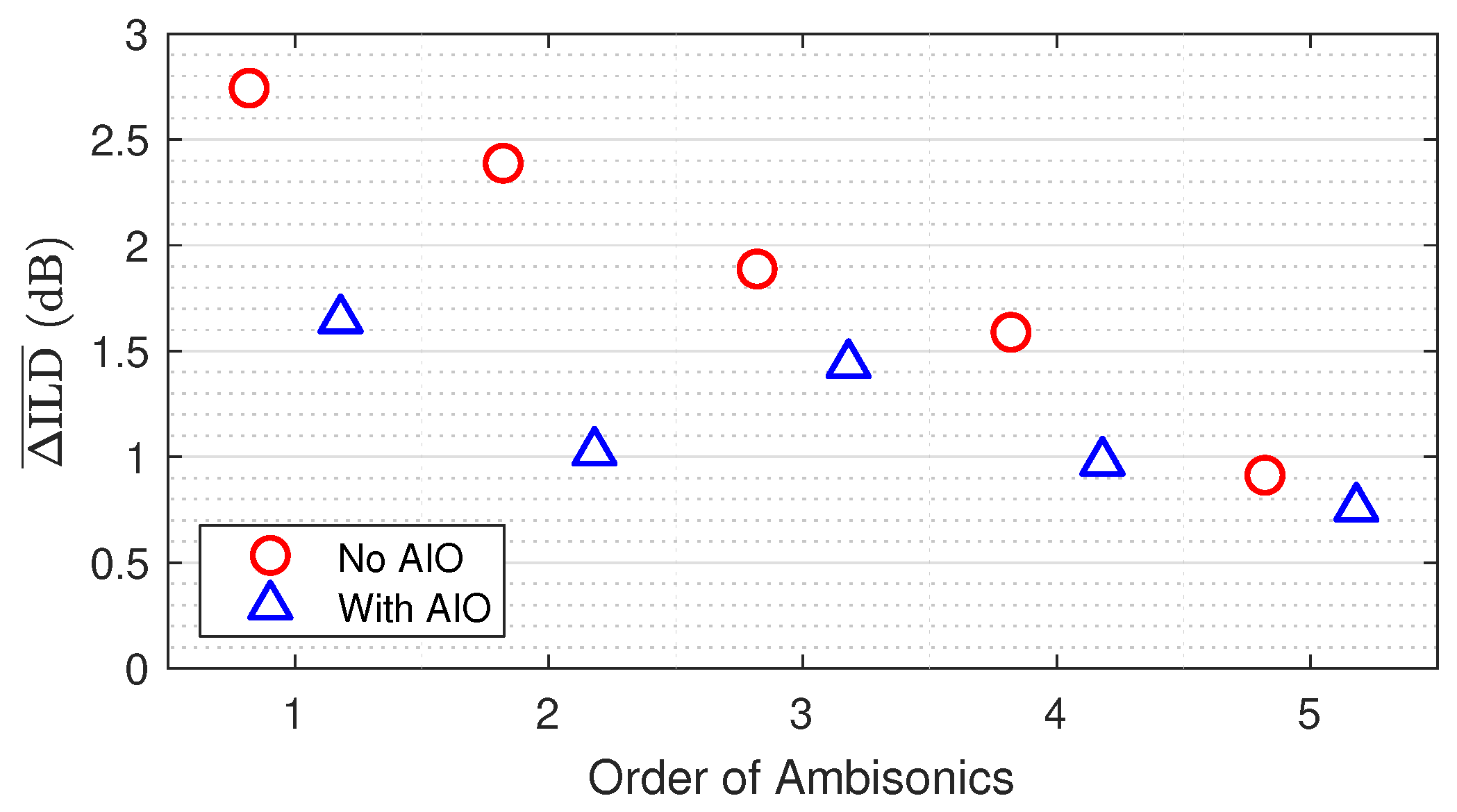
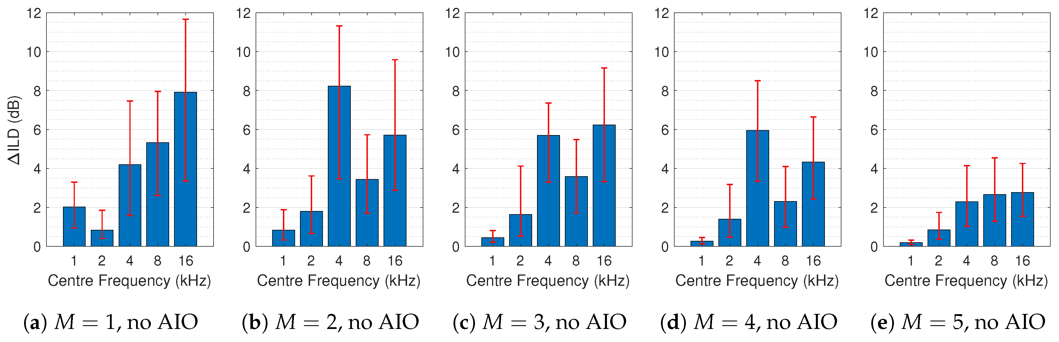
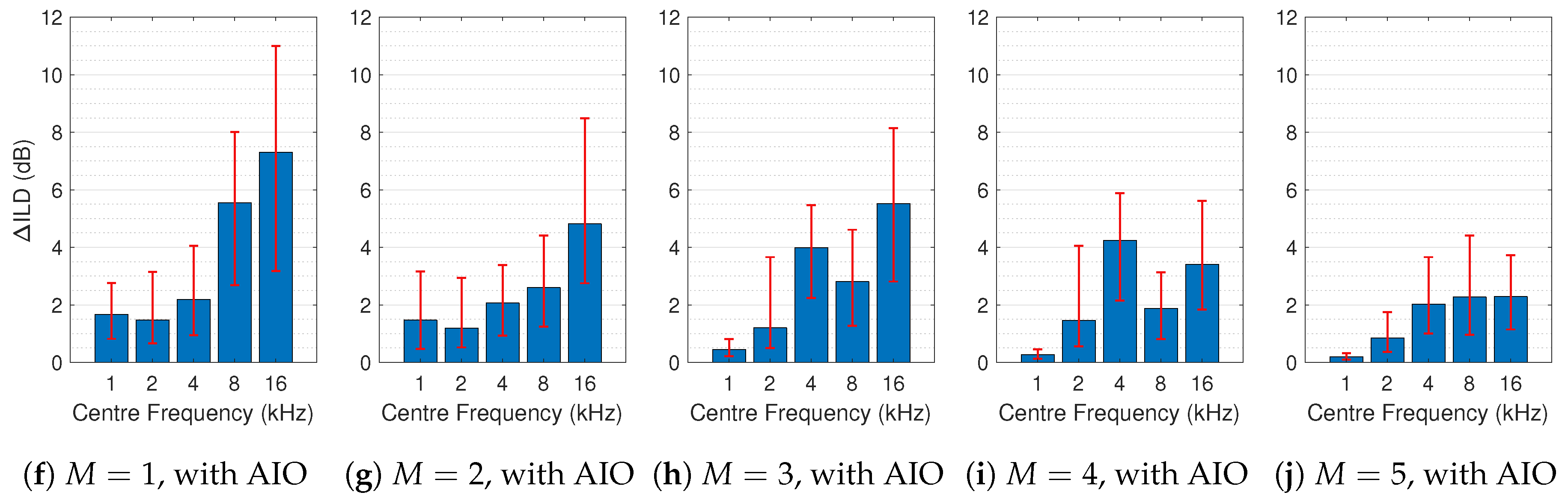
The effect of AIO has been evaluated both objectively and perceptually. Theoretically, perfect Ambisonic reproduction would produce binaural Ambisonic rendered HRIRs equivalent to non-Ambisonic rendered HRIRs. Objective evaluation therefore compared binaural Ambisonic rendered HRIRs, both without and with AIO, to a reference dataset of HRIRs. Evaluation metrics used were accuracy of rendered ILD, both over all directions on the sphere and over frequency, and spectral difference.
The high-resolution reference HRIR dataset used was chosen as the 2 Gauss-Legendre quadrature of the Bernschütz Neumann KU 100 HRIR database [40], which features measurements of 89 elevations at 180 different azimuth values in 2 increments, totaling 16,020 measurements. The reference dataset is herein referred to as H . Figure 4 plots the vertices of an 8 Gauss-Legendre quadrature with 23 elevations at 45 different azimuth values in 8 increments totaling 1035 points (a lower resolution than the 2 Gauss-Legendre quadrature used in the evaluation to aid visibility). Shading is based on the solid angle (denoted in this paper as Ω ) of each point, which is calculated from the area of the sphere for which a single point subtends [42], such that Ω = 1 . Figure 4 illustrates the clustering of points at the poles in Gauss-Legendre quadrature, and thus the need for solid-angle weighting in calculations when obtaining a single value over all locations on the sphere in this paper.
For each of the measurement locations { ϱ 1 , ϱ 2 , , ϱ 16,020 } of H , Ambisonic gains were encoded and decoded binaurally for Ambisonic orders { M = 1 , M = 2 , , M = 5 } to create corresponding datasets of Ambisonic rendered HRIRs H ^ , both standard binaural Ambisonic rendering ( H ^ s t d ) and binaural Ambisonic rendering with AIO pre-processed HRIRs ( H ^ A I O ).

3.1. Change in ILD

To assess the effect of AIO on binaural Ambisonic ILD reproduction, the ILD of all datasets: H , H ^ s t d and H ^ A I O was estimated for all measurement locations { ϱ 1 , ϱ 2 , , ϱ 16,020 } and orders of Ambisonics { M = 1 , M = 2 , , M = 5 } according to (8). The absolute difference between the estimated ILD values for each measurement location was then calculated as
Δ ILD ϱ = | ILD ( H ϱ ) ILD ( H ^ ϱ ) |
Figure 5 shows Δ ILD for all measurement locations over the left hemisphere, both without (top) and with (bottom) AIO, for orders of Ambisonics { M = 1 , M = 2 , , M = 5 }. Smaller values of Δ ILD indicate ILD rendering closer to the HRIR. It is clear that ILD is improved for most locations on the sphere, for all tested orders of Ambisonics, though the effect is most pronounced at first and second order.
A single value of Δ ILD for all locations on the sphere, Δ ILD ¯ , was calculated from the solid-angle weighted sum of all Δ ILD values as
Δ ILD ¯ = ϱ = 1 16020 Ω ϱ Δ ILD ϱ
Values of Δ ILD ¯ for orders of Ambisonics { M = 1 , M = 2 , , M = 5 } are presented in Figure 6. This shows that with AIO, ILD is reproduced with greater accuracy for all tested orders of Ambisonics; indeed, a greater accuracy than M + 1 without AIO for all tested orders apart from the M = 4 instance. The improvement is greatest at orders M = 1 and M = 2 though, where Ambisonic ILD reproduction is inherently the least accurate.
To look closer at Δ ILD between binaural Ambisonic rendering and HRIRs, a second ILD calculation was made to observe how Δ ILD changes with frequency. Instead of producing one value of ILD for all frequencies using 30 ERB bands as in (8), ILD was calculated separately for 5 frequency bands with center frequencies of 1 kHz, 2 kHz, 4 kHz, 8 kHz and 16 kHz. Figure 7 illustrates the median value of Δ ILD over all measurement locations { ϱ 1 , ϱ 2 , , ϱ 16,020 } between H and H ^ for Ambisonic orders { M = 1 , M = 2 , , M = 5 }, both without (top) and with (bottom) AIO, across 5 frequency bands. 25% and 75% percentile bars are included to demonstrate the divergence from the median. Observations of the graph show that in general, Δ ILD between binaural Ambisonic rendering and HRIRs increases with frequency, and AIO improves ILD reproduction over all frequency bands fairly evenly.

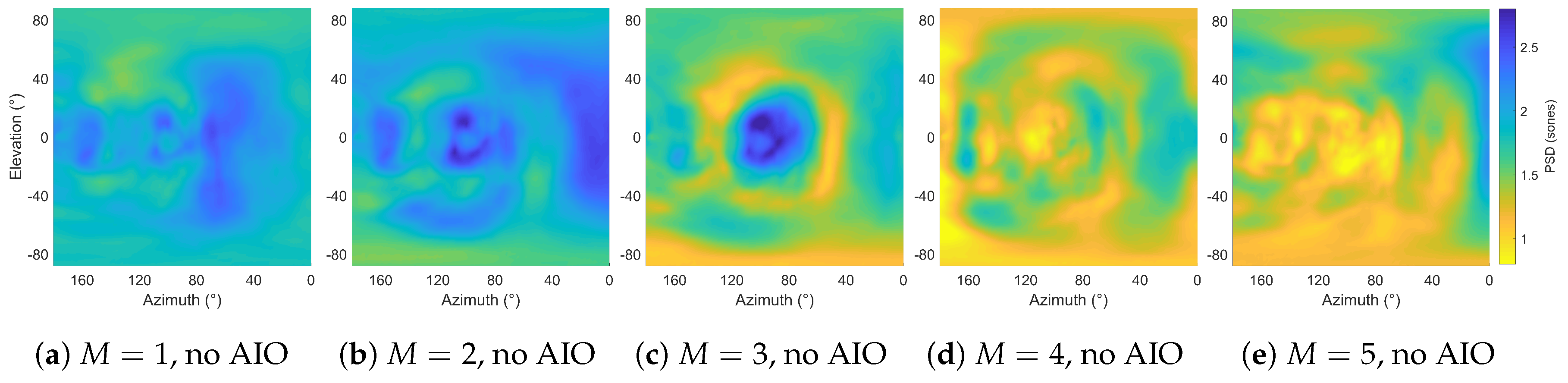
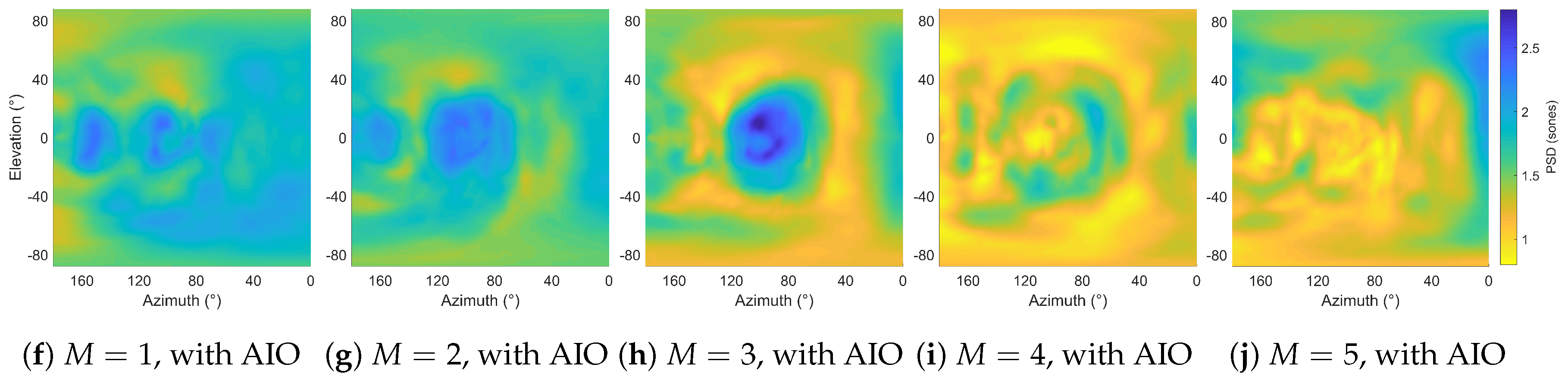
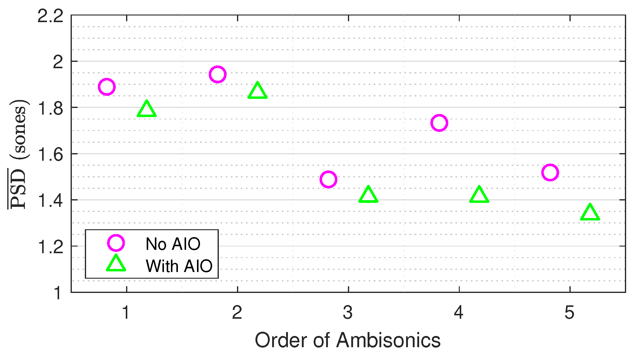
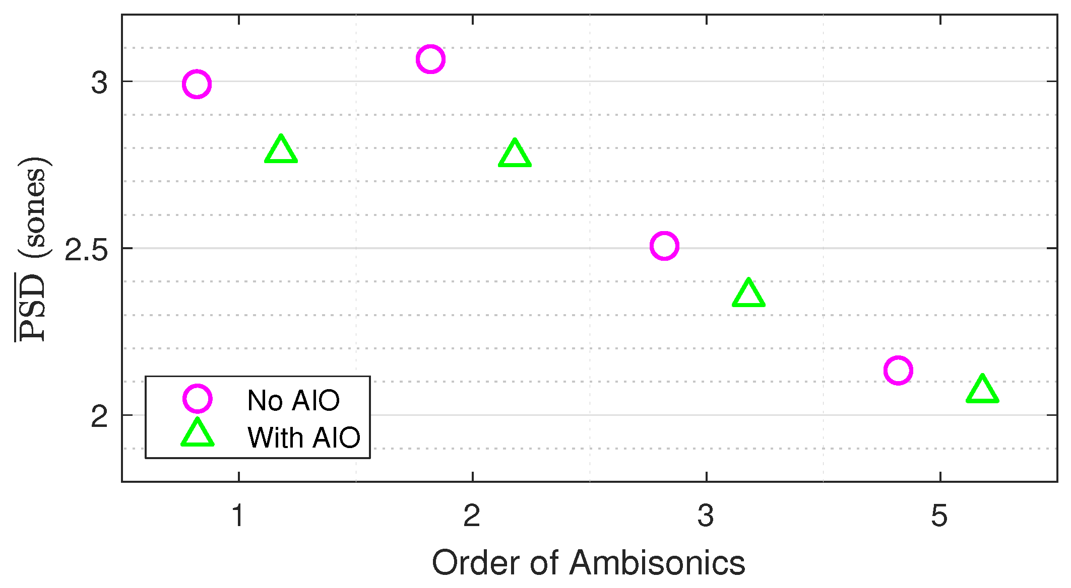
3.2. Spectral Difference

To assess the effect of AIO on spectral reproduction of Ambisonic signals, a perceptual FFT-based spectral difference (PSD) model was used that takes into account various features of human auditory perception [43]. The PSD model weights input signals using ISO 226 equal loudness contours [44] to account for the frequency-varying sensitivity of human hearing, with a sone scale to account for the loudness-varying sensitivity of human hearing, and ERB weightings to address how the linearly spaced samples of an FFT do not fairly represent the approximately logarithmic sensitivity of the inner ear. For each measurement location, PSD was taken as the absolute mean of the left and right calculations:
PSD = | PSD l e f t + PSD r i g h t 2 |
PSD between H and H ^ was calculated for all measurement locations { ϱ 1 , ϱ 2 , , ϱ 16,020 }, for Ambisonic orders { M = 1 , M = 2 , , M = 5 }, both without and with AIO. Figure 8 shows PSD values for Ambisonic orders { M = 1 , M = 2 , , M = 5 } over all locations on the left hemisphere, both without (top) and with (bottom) AIO. A small improvement in most measurement locations can be observed. Binaural Ambisonic rendering is known to produce differences in spectral reproduction accuracy between front and side, something which is illustrated in Figure 8 (especially for M = 2 and M = 3 , Figure 8b,c, respectively). While the implementation of AIO does reduce this to some extent, it is still evident.
A single value of PSD for all locations on the sphere, PSD ¯ , was obtained as the solid-angle weighted sum of all PSD values by
PSD ¯ = ϱ = 1 16020 Ω ϱ PSD ϱ
The PSD ¯ values for Ambisonic orders { M = 1 , M = 2 , , M = 5 }, without and with AIO, are presented in Figure 9. Here AIO is shown to produce an overall improvement in PSD for all tested orders of Ambisonics.

3.3. Generalizability

To demonstrate the robust applicability of AIO, additional simulations were run using both different loudspeaker configurations and a different HRIR dataset. In both sets of simulations, the effect of AIO was assessed as in Section 3.2, with PSD calculations comparing Ambisonic renders to the original HRIRs for all available measurement locations according to (17) and single values of PSD ¯ then calculated from (18).
The first looked at different loudspeaker configurations. For all other aspects of this paper, AIO has been applied to Lebedev loudspeaker configurations. Here, another common Ambisonic loudspeaker configuration was used: spherical T-designs [45]. For each Ambisonic order { M = 1 , M = 2 , , M = 5 }, T-designs corresponding to { L = 8 , L = 12 , L = 24 , L = 48 , L = 70 } were used respectively, fulfilling the orthonormality requirement T 2 M + 1 [46]. The PSD ¯ results, calculated from 16,020 locations on the sphere, are shown in Figure 10. This illustrates how AIO produces an overall improvement in PSD, regardless of the type of loudspeaker configuration.
Secondly, to assess how AIO works when using other HRIR datasets, renders were made for { M = 1 , M = 2 , M = 3 , M = 5 } using individualized HRIRs from human subject H20 of the SADIE II database [47], using the corresponding Lebedev loudspeaker configurations as before. The omission of M = 4 was due to a lack of necessary measurements. The PSD ¯ results, calculated from 2114 locations on the sphere, are shown in Figure 11. This illustrates how, again, AIO produces an overall improvement in PSD for all tested orders of Ambisonics, regardless of the HRIR database or subject used.
The tests on generalizability show that AIO improves the spectral reproduction of binaural Ambisonic rendering for all virtual loudspeaker configurations, regardless of Ambisonic order or HRIR dataset. However, the magnitude of improvement has been shown to vary with loudspeaker configuration, as shown by the differences between Figure 9 and Figure 10. A trend appears to exist between loudspeaker configurations regardless of HRIR dataset, as shown by the similarities between Figure 9 and Figure 11.

4. Perceptual Evaluation

To assess the perceptual effect of AIO in binaural Ambisonic rendering, two listening tests were conducted, corresponding to simple acoustic scenes and complex acoustic scenes. In this paper, a simple scene refers to a sound scene with a single point source at a fixed location and distance, and a complex scene refers to a sound scene with multiple sources of varying source widths, locations, and distances. Simple scenes are appropriate for evaluating the finer perceptual differences between audio systems in highly controlled listening scenarios, whereas complex scenes are appropriate for simulating a listening scenario closer to real-life. As the objective evaluation showed AIO to produce the most notable effects for low-order Ambisonics (in particular, M = 1 and M = 2 ), the perceptual evaluation focused on low-order ( M < 5 ) rendering.
Listening tests were conducted on 18 participants aged between 23 to 71. The demographic followed 14 male, 3 female, 1 non-binary. All reported normal hearing as in accordance with ISO Standard 389 [48] and prior critical listening experience, which was deemed sufficient if the participant had education or employment in audio or music engineering.

4.1. Test Methodologies

Tests were conducted in a quiet room using an Apple MacBook Pro with a Fireface 400 audio interface, which has software-controlled input and output levels. All binaural renders were static (fixed head orientation) to ensure consistency in the experience between participants. A single set of Sennheiser HD 650 circum-aural headphones was used for all tests, which were equalized using a Neumann KU 100 dummy head from 11 measurements using the exponential swept sine impulse response technique [49] with re-fitting of the headphones between each measurement. Equalization filters were calculated from the RMS average of the 11 measured headphone transfer functions (HpTFs) using Kirkeby and Nelson’s least-mean-square regularization method [50], which has been shown to produce perceptually superior equalization when compared to other currently available methods [51]. One octave smoothing was implemented using the complex smoothing approach of [52], and the range of inversion was 5 Hz–4 kHz. In-band and out-band regularization of 25 dB and −2 dB respectively was used, to avoid sharp peaks in the inverse filter which are more noticeable than notches [53]. The RMS HpTF and inverse filter of the left HD 650 headphone, along with a resulting convolved response, are shown in Figure 12.

4.1.1. Simple Scenes

The first listening test assessed the perceptual effect of AIO in binaural Ambisonic rendering for simple scenes. The base stimulus was a one second burst of monophonic pink noise at a sample rate of 48 kHz, windowed by onset and offset half-Hanning ramps of 5 ms, with half a second of silence between each burst. Test sound locations ψ were chosen as the central points of the faces of a dodecahedron, to avoid test sound locations coinciding with loudspeaker locations. To reduce the total number of trials, symmetry was assumed leaving only locations in the left hemisphere or on the median plane. Table 1 displays the spherical coordinates of each test sound location.
The simple-scenes listening test followed the multiple stimulus with hidden reference and anchors (MUSHRA) paradigm, ITU-R BS.1534-3 [54]. The reference was a direct HRIR convolution, the medium anchor was a low-pass filtered version of the reference with an f c = 7 kHz, and the low anchor was the monophonic base stimulus low-pass filtered at an f c = 3.5 kHz. The other 6 stimuli were binaural Ambisonic renders for three Ambisonic orders { M = 1 , M = 2 , M = 3 }, without and with AIO, totaling 9 test stimuli per trial. For each trial, the listener was asked to rate the 9 stimuli with a score between 0 and 100 in terms of overall perceived similarity to the reference, in accordance with the Spatial Audio Quality Inventory (SAQI) [55] whereby increased similarity would be rated higher. Each trial was repeated once, giving a total of 16 trials. Stimuli and trial ordering was randomized and presented double blind.

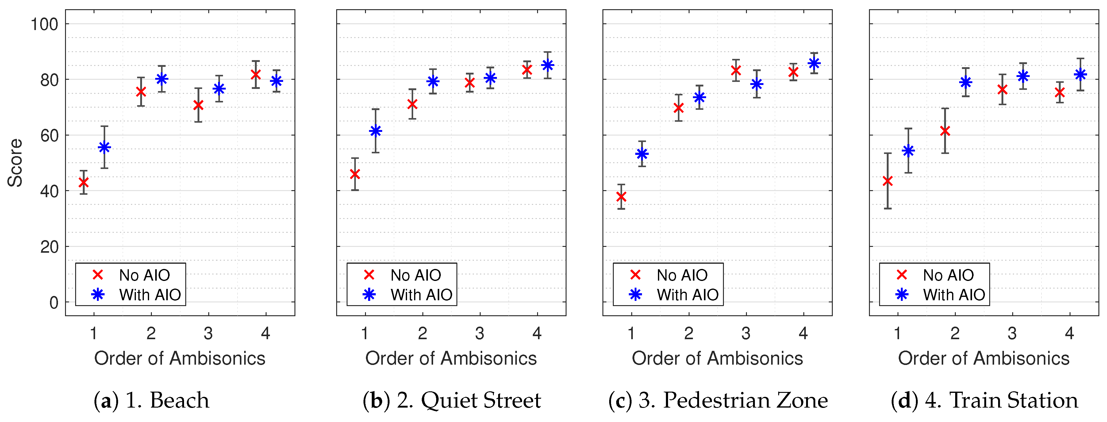
4.1.2. Complex Scenes

The second listening test used four complex scenes, which were 3–5 second excerpts of soundscape recordings from the open source EigenScape database of fourth-order Ambisonic recordings made using an mh acoustics em32 EigenMike at various locations in northern England [56]. The initial format of recordings follows Schmidt semi-normalized (SN3D) normalization, which therefore was converted to N3D normalization by
β k N 3 D = 2 m + 1 β k S N 3 D
The soundscapes used in this listening test, along with a description of the specific excerpt used are as follows:
  • Beach (waves breaking against the shore)
  • Quiet Street (a single car drives past with birdsong)
  • Pedestrian Zone (pedestrians walking around and talking)
  • Train Station (travel announcement on the station platform)
The composition of scenes featured mainly horizontal sounds, though elevated sources were present such as the birdsong in scene 2 and travel announcement in scene 4, as well as the room reverberation in scene 3 and 4 due to the recordings having been made indoors.
The complex-scenes listening test loosely followed the MUSHRA paradigm [54]; however, due to the nature of the stimuli no ideal reference was available. Partly for this reason, the M = 4 renders were included in the complex-scenes test which are the highest available Ambisonic order of EigenMike recordings. Lower-order renders were obtained by simply discarding the higher-order channels. An M = 0 render was used as an anchor, and test stimuli were binaural Ambisonic renders for orders { M = 1 , M = 2 , , M = 4 }, without and with AIO, totaling 9 test stimuli per trial. For each trial, participants were asked to rate each stimuli with a score between 0 and 100 on plausibility and spaciousness, whereby natural, wide, full and externalized stimuli would be rated higher, and boxed in, lacking lateralization, internalized stimuli would be rated lower. Each trial was repeated once, giving a total of 8 trials. Stimuli and trial ordering was again randomized and presented double blind.

4.2. Results

Results were post-screened for unreliable participants based on the following criteria. For simple scenes: rating the hidden reference lower than 90% for >15% of trials or rating the mid-anchor higher than 90% for >15% of trials, and for complex scenes: rating the anchor higher than 90% for >15% of trials. Based on these criteria, one participant’s results were excluded from analysis. The raw results from both listening tests were tested for normality using the Kolmogorov-Smirnov test, which showed all data as non-normally distributed. Therefore, all statistical analysis was conducted using non-parametric methods.

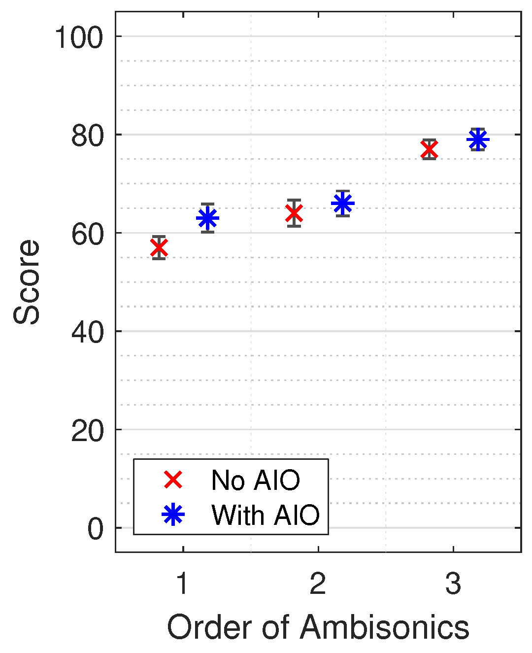
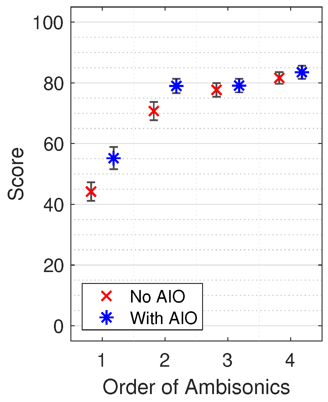
4.2.1. Simple Scenes

The median scores of the simple-scenes test, conducted to determine whether AIO improves the overall perceived similarity between binaural Ambisonic rendering and HRIR convolution, are shown in Figure 13 for each order of Ambisonics across all participants and test sound locations, with non-parametric 95% confidence intervals (CI) [57] (reference and anchor scores are omitted). The different conditions of the test were tested for statistical significance using a Friedman’s analysis of variance (ANOVA) test, which showed statistical significance ( χ 2 ( 5 ) = 203.71 , p < 0.01 ). From the figure, AIO is shown to produce an increase in overall perceived similarity for all tested orders of Ambisonics. To test whether this improvement is statistically significant, Wilcoxon signed-rank tests were conducted for each Ambisonic order, and Table 2 presents the significance results. For M = 1 and M = 2 , AIO produced a statistically significant improvement in overall perceived similarity between binaural Ambisonic rendering and HRIR convolution. Though an improvement can be observed for M = 3 , it was not statistically significant at a confidence of 95%.
To assess whether the perceptual effect of AIO varied with test sound location, a Friedman’s ANOVA was conducted, which showed high statistical significance ( χ 2 ( 7 ) = 39.61 , p < 0.01 ). Figure 14 illustrates the median scores with non-parametric 95% CI for each individual test sound location ψ across all participants. Post-hoc Wilcoxon signed-rank tests were conducted to determine which test sound locations produced a significant improvement in overall perceived similarity for AIO, the results of which are shown in Table 3. It is clear that results varied for test sound location differently for each tested Ambisonic order. Additionally, some participants noted minor listening fatigue in the simple scenes due to repeated pink noise bursts, so future tests should look at addressing this.

4.2.2. Complex Scenes

The median scores of the complex-scenes test, conducted to determine whether AIO improves plausibility and spaciousness of binaural Ambisonic rendering, are shown in Figure 15 for each condition across all participants and test sound locations, with non-parametric 95% CI [57]. A Friedman’s ANOVA confirmed that the test conditions produced statistically significantly different results ( χ 2 ( 7 ) = 264.4 , p < 0.01 ). An observation of Figure 15 indicates that ratings increase with Ambisonic order, tapering off as order increases, and AIO improves the ratings for all tested orders, though the improvement is greatest at M = 1 and M = 2 . To test whether this improvement for each order is statistically significant, Wilcoxon signed-rank tests were conducted. Table 4 presents the significance results. For M = 1 and M = 2 , AIO produces a statistically significant improvement. Though improvements are still observed for M = 3 and M = 4 , they are not statistically significant at 95% confidence ( p = 0.1 and p = 0.07 , respectively).
Figure 16 shows the median scores with non-parametric 95% CI across all participants for each individual soundscape. AIO produced a higher median score than without AIO for all soundscapes and tested orders, apart from the conditions of M = 4 soundscape 1 and M = 3 soundscape 3. To observe whether soundscape type had a statistically significant effect on results, a Friedman’s ANOVA was conducted, which showed no significance ( χ 2 ( 3 ) = 1.9 , p = 0.59 ).

5. Discussion

The evaluation showed that AIO successfully improves the ILD reproduction of virtual loudspeaker binaural Ambisonic rendering, when compared to HRIRs. In most cases this comes in the form of an increase in ILD, but not all - some places show AIO reduces ILD of the Ambisonic rendering. The evaluation of the AIO algorithm in ILD reproduction for all directions over the sphere showed that AIO improves ILD reproduction for all tested Ambisonic orders. Though AIO improved ILD reproduction even at M = 5 , the greatest benefits were obtained where ILD is inherently reproduced the worst: at M = 1 and M = 2 .
Where AIO produced greater improvements in ILD reproduction, more substantial improvements were also observed in PSD and listening test results. M = 2 produced the largest improvement in ILD reproduction over the sphere, and this was followed by the biggest improvement in PSD. With AIO, M = 2 had ILD reproduction better than M = 3 , and PSD and listening test results were close to M = 3 .
In general, Δ ILD between HRIRs and binaural Ambisonic rendering has been shown to increase with frequency, as illustrated in Figure 7. This is likely caused by Ambisonic spatial aliasing, which increases with frequency once above f a l i a s . Implementing AIO reduces Δ ILD relatively evenly over all frequency bands, which is likely a result of the AIO algorithm only producing a single gain value for all frequencies. Therefore, implementing frequency specific ILD optimization in a future development, for example, could possibly produce further improvements.
Concerning the listening test results, AIO produced notable improvements for M = 1 and M = 2 , and small (but generally not statistically significant) improvements for M = 3 and M = 4 . However, in the simple-scenes test, sound source location was found to be a significant influence on results. In the complex-scenes listening test, the type of soundscape did not affect results with statistical significance. An interesting overall observation is the stark differences between simple and complex-scene results. There was a much greater difference observed in scores between Ambisonic orders in complex scenes, and AIO produced more significant improvements here. Pink noise, used in the simple-scenes tests, focuses the listener on timbre, whereas recorded soundscapes of complex acoustic scenes have more of a focus on lateralization and spaciousness due to the numerous simultaneous sources. Further investigation is warranted to conclude the reason for the variation in results between the two tests.
Some further observations were made during this study. Despite the iterative pre-processing stage, the ILD augmentation gains for M = 1 plateaued, causing the Ambisonic reproduced ILDs to not quite reach those of the HRIR targets (see Figure 3a). This is due to the normalization of HRIRs post-AIO processing using (13), which normalizes the processed HRIR to the same RMS as the unprocessed HRIR. With this normalization, the contralateral signal of the HRIRs with AIO processing for M = 1 had a very low amplitude (they were essentially muted). Therefore, a further increase in ILD did not produce any change in results. Some preliminary experimentation found that if the normalization was changed such that HRIRs with AIO were normalized with respect to the RMS amplitude of the Ambisonically reproduced HRIR, AIO HRIRs could then become much louder than unprocessed (median plane) HRIRs, which can produce Ambisonic ILDs much greater. However, this comes at the expense of spectral quality on the median plane. As median plane accuracy is of great importance [58], the initial normalization method was retained.
Though most simulations in this paper concerned Lebedev loudspeaker configurations and a single HRIR dataset, additional simulations on generalizability of the results revealed that AIO is applicable for all HRIR datasets and loudspeaker configurations. Therefore, a general statement can be suggested that for virtual loudspeaker binaural Ambisonic rendering, AIO offers a clear improvement for first and second order Ambisonics.

6. Conclusions and Future Work

ILD reproduction of binaural Ambisonic rendering has been shown as inaccurate at low orders of Ambisonics. This paper has presented a method for Ambisonic interaural level difference optimization, aiming to improve the ILD reproduction of low-order binaural Ambisonic rendering using virtual loudspeakers. This has been achieved through an iterative pre-processing stage whereby the ILD of the HRIRs for binaural rendering are measured and then augmented accordingly at frequencies above f a l i a s by applying a gain to the contralateral signal of the HRIR such that when used for binaural Ambisonic rendering, the resulting rendered ILD matches that of the original HRIR more closely.
The effect of AIO has been evaluated both objectively and perceptually. Objective evaluation compared binaural Ambisonic rendering, both without and with AIO, to HRIR references for Ambisonic orders { M = 1 , M = 2 , , M = 5 } in three ways: change in ILD, both over direction and over frequency, and spectral difference over all directions on the sphere. In all three, AIO was shown to produce overall improvements, with greater improvements in ILD reproduction being shown to produce the most significant improvements in spectral reproduction. Perceptual evaluation in the form of listening tests using both simple and complex acoustic scenes largely corroborated the results of the objective evaluation. General findings showed AIO is most effective at M = 1 and M = 2 where Ambisonic ILD reproduction is inherently the least accurate. Implementing AIO produces an improvement in lateralization, which helps to reduce the perceptual differences between orders. As AIO pre-processing of HRIRs can be implemented offline, it is hence recommended for improving lateralization and spaciousness for all orders of Ambisonics, without producing a reduction in timbral quality.
Future work will look at adapting the AIO algorithm to implement frequency-dependent gains for each loudspeaker instead of a single gain as is the current case. Planned subsequent work will also look at integrating the presented AIO method with other pre-processing techniques for improving high-frequency reproduction of binaural Ambisonic rendering using virtual loudspeakers, such as diffuse-field equalization [59], direction-bias equalization [58] and time-alignment [25,26,27]. Preliminary tests have shown that combining AIO with these equalization methods can produce even greater improvements to high-frequency reproduction, and possibly allow for the perceptual experience of a higher Ambisonic order without an increase in convolutions. Finally, comparisons with other state-of-the-art pre-processing techniques such as magnitude least squares [28] will be made, both objectively and perceptually.

Author Contributions

Conceptualization, T.M. and G.K.; Methodology, T.M.; Software, T.M.; Validation, T.M., D.T.M. and G.K.; Formal Analysis, T.M.; Investigation, T.M.; Resources, T.M.; Data Curation, T.M.; Writing—Original Draft Preparation, T.M.; Writing—Review & Editing, T.M., D.T.M. and G.K.; Visualization, T.M.; Supervision, D.T.M. and G.K.; Project Administration, T.M.; Funding Acquisition, G.K.

Funding

This research was supported by a Google Faculty Research Award and the Engineering and Physical Sciences Research Council (EP/M001210/1).

Conflicts of Interest

The authors declare no conflict of interest. The founding sponsors had no role in the design of the study; in the collection, analyses, or interpretation of data; in the writing of the manuscript, and in the decision to publish the results.

References

  1. Blauert, J. Spatial Hearing: The Psychophysics of Human Sound Localization; MIT Press: Cambridge, MA, USA, 1997. [Google Scholar]
  2. Lindau, A.; Weinzierl, S. Assessing the plausibility of virtual acoustic environments. Acta Acust. United Acust. 2012, 98, 804–810. [Google Scholar] [CrossRef]
  3. Brinkmann, F.; Lindau, A.; Weinzierl, S. On the authenticity of individual dynamic binaural synthesis. J. Acoust. Soc. Am. 2017, 142, 1784–1795. [Google Scholar] [CrossRef] [Green Version]
  4. Wenzel, E.; Arruda, M.; Kistler, D.; Wightman, F.L. Localization using nonindividualized head-related transfer functions. J. Acoust. Soc. Am. 1993, 94, 111–123. [Google Scholar] [CrossRef] [PubMed]
  5. Møller, H.; Sørensen, M.F.; Jensen, C.B.; Hammershøi, D. Binaural technique: Do we need individual recordings? J. Audio Eng. Soc. 1996, 44, 451–469. [Google Scholar]
  6. Lindau, A.; Maempel, H.; Weinzierl, S. Minimum BRIR grid resolution for dynamic binaural synthesis. In Proceedings of the Acoustics 08 Paris, Paris, France, 30 June–4 July 2008; pp. 3851–3856. [Google Scholar]
  7. Gerzon, M.A. Periphony: With-height sound reproduction. J. Audio Eng. Soc. 1973, 21, 2–10. [Google Scholar]
  8. Gerzon, M.A. Criteria for evaluating surround-sound systems. J. Audio Eng. Soc. 1977, 25, 400–408. [Google Scholar]
  9. Malham, D.; Myatt, A. 3-D sound spatialization using Ambisonic techniques. Comput. Music J. 1995, 19, 58–70. [Google Scholar] [CrossRef]
  10. Poletti, M. The Design of Encoding Functions for Stereophonic and Polyphonic Sound Systems. J. Audio Eng. Soc. 1996, 44, 948–963. [Google Scholar]
  11. Moreau, S.; Daniel, J.; Bertet, S. 3D Sound Field Recording With Higher Order Ambisonics-Objective Measurements and Validation of a 4th Order Spherical Microphone. In Proceedings of the 120th Convention of the Audio Engineering Society, Paris, France, 20–23 May 2006. [Google Scholar]
  12. Bertet, S.; Daniel, J.; Parizet, E.; Warusfel, O. Investigation on localisation accuracy for first and higher order Ambisonics reproduced sound sources. Acta Acust. United Acust. 2013, 99, 642–657. [Google Scholar] [CrossRef]
  13. Jot, J.M.; Larcher, V.; Pernaux, J.M. A comparative study of 3-D audio encoding and rendering techniques. In Proceedings of the AES 16th International Conference: Spatial Sound Reproduction, Rovaniemi, Finland, 10–12 April 1999; pp. 281–300. [Google Scholar]
  14. Daniel, J.; Rault, J.B.; Polack, J.D. Ambisonics encoding of other audio formats for multiple listening conditions. In Proceedings of the 105th Convention of the Audio Engineering Society, San Francisco, CA, USA, 26–29 September 1998. [Google Scholar]
  15. Bamford, J.S.; Vanderkooy, J. Ambisonic Sound for Us. In Proceedings of the 99th Convention of the Audio Engineering Society, New York, NY, USA, 6–9 October 1995. [Google Scholar]
  16. Malham, D.G. Higher order Ambisonic systems for the spatialisation of sound. Proc. ICMC 1999, 1999, 484–487. [Google Scholar]
  17. Collins, T. Binaural Ambisonic decoding with enhanced lateral localization. In Proceedings of the 134th Convention of the Audio Engineering Society, Rome, Italy, 4–7 May 2013. [Google Scholar]
  18. Yao, S.N.; Collins, T.; Jančovič, P. Timbral and spatial fidelity improvement in ambisonics. Appl. Acoust. 2015, 93, 1–8. [Google Scholar] [CrossRef]
  19. Jot, J.M.; Wardle, S.; Larcher, V. Approaches to binaural synthesis. In Proceedings of the 105th Convention of the Audio Engineering Society, San Francisco, CA, USA, 26–29 September 1998. [Google Scholar]
  20. Noisternig, M.; Sontacchi, A.; Musil, T.; Höldrich, R. A 3D ambisonic based binaural sound reproduction system. In Proceedings of the AES 24th International Conference on Multichannel Audio, Banff, AB, Canada, 26–28 June 2003. [Google Scholar]
  21. Avni, A.; Ahrens, J.; Geier, M.; Spors, S.; Wierstorf, H.; Rafaely, B. Spatial perception of sound fields recorded by spherical microphone arrays with varying spatial resolution. J. Acoust. Soc. Am. 2013, 133, 2711–2721. [Google Scholar] [CrossRef] [PubMed]
  22. Bernschütz, B.; Vázquez Giner, A.; Pörschmann, C.; Arend, J. Binaural reproduction of plane waves with reduced modal order. Acta Acust. United Acust. 2014, 100, 972–983. [Google Scholar] [CrossRef]
  23. Brinkmann, F.; Weinzierl, S. Comparison of head-related transfer functions pre-processing techniques for spherical harmonics decomposition. In Proceedings of the AES Conference on Audio for Virtual and Augmented Reality, Redmond, WA, USA, 20–22 August 2018. [Google Scholar]
  24. Ben-Hur, Z.; Brinkmann, F.; Sheaffer, J.; Weinzierl, S.; Rafaely, B. Spectral equalization in binaural signals represented by order-truncated spherical harmonics. J. Acoust. Soc. Am. 2017, 141, 4087–4096. [Google Scholar] [CrossRef] [PubMed]
  25. Evans, M.J.; Angus, J.A.S.; Tew, A.I. Analyzing head-related transfer function measurements using surface spherical harmonics. J. Acoust. Soc. Am. 1998, 104, 2400–2411. [Google Scholar] [CrossRef]
  26. Richter, J.G.; Pollow, M.; Wefers, F.; Fels, J. Spherical harmonics based HRTF datasets: Implementation and evaluation for real-time auralization. Acta Acust. United Acust. 2014, 100, 667–675. [Google Scholar] [CrossRef]
  27. Zaunschirm, M.; Schörkhuber, C.; Höldrich, R. Binaural rendering of Ambisonic signals by HRIR time alignment and a diffuseness constraint. J. Acoust. Soc. Am. 2018, 143, 3616–3627. [Google Scholar] [CrossRef] [PubMed]
  28. Schörkhuber, C.; Zaunschirm, M.; Höldrich, R. Binaural rendering of Ambisonic signals via Magnitude Least Squares. In Proceedings of the DAGA 2018: 44. Deutsche Jahrestagung für Akustik, Munich, Germany, 19–22 March 2018; pp. 339–342. [Google Scholar]
  29. Lebedev, V.I. Quadratures on a sphere. USSR Comput. Math. Math. Phys. 1976, 16, 10–24. [Google Scholar] [CrossRef]
  30. Zotkin, D.N.; Duraiswami, R.; Grassi, E.; Gumerov, N.A. Fast head-related transfer function measurement via reciprocity. J. Acoust. Soc. Am. 2006, 120, 2202–2215. [Google Scholar] [CrossRef] [PubMed]
  31. Majdak, P.; Balazs, P.; Laback, B. Multiple exponential sweep method for fast measurement of head-related transfer functions. J. Audio Eng. Soc. 2007, 55, 623–636. [Google Scholar]
  32. Abramowitz, M.; Stegun, I. Handbook of Mathematical Functions, 10th ed.; Dover Publications: Washington, DC, USA, 1972. [Google Scholar]
  33. Heller, A.J.; Lee, R.; Benjamin, E.M. Is my decoder ambisonic? In Proceedings of the 125th Convention of the Audio Engineering Society, San Francisco, CA, USA, 2–5 October 2008. [Google Scholar]
  34. Gerzon, M.A.; Barton, G.J. Ambisonic decoders for HDTV. In Proceedings of the 92nd Convention of the Audio Engineering Society, Vienna, Austria, 24–27 March 1992. [Google Scholar]
  35. Daniel, J. Représentation de Champs Acoustiques, Application à la Transmission et à la Reproduction De Scènes Sonores Complexes Dans un Contexte Multimédia. Ph.D. Thesis, l’Université Pierre et Marie Curie, Paris, France, 2000. [Google Scholar]
  36. Harris, F.J. Multirate Signal Processing for Communication Systems; Prentice Hall PTR: Upper Saddle River, NJ, USA, 2004. [Google Scholar]
  37. Lecomte, P.; Gauthier, P.A.; Langrenne, C.; Berry, A.; Garcia, A. A fifty-node Lebedev grid and its applications to Ambisonics. J. Audio Eng. Soc. 2016, 64, 868–881. [Google Scholar] [CrossRef]
  38. Thresh, L.; Armstrong, C.; Kearney, G. A direct comparison of localisation performance when using first, third and fifth order Ambisonics for real loudspeaker and virtual loudspeaker rendering. In Proceedings of the Audio Engineering Society Convention 143, New York, NY, USA, 18–20 October 2017. [Google Scholar]
  39. Burkardt, J. SPHERE_LEBEDEV_RULE—Quadrature Rules for the Unit Sphere. Available online: http://people.sc.fsu.edu/~jburkardt/datasets/sphere_lebedev_rule/sphere_lebedev_rule.html (accessed on 15 February 2019).
  40. Bernschütz, B. A spherical far field HRIR/HRTF compilation of the Neumann KU 100. In Proceedings of the Fortschritte der Akustik—AIA-DAGA 2013, Merano, Italy, 18–21 March 2013; pp. 592–595. [Google Scholar]
  41. Watanabe, K.; Ozawa, K.; Iwaya, Y.; Suzuki, Y.; Aso, K. Estimation of interaural level difference based on anthropometry and its effect on sound localization. J. Acoust. Soc. Am. 2007, 122, 2832–2841. [Google Scholar] [CrossRef] [PubMed]
  42. Oosterom, A.V.; Strackee, J. The solid angle of a plane triangle. IEEE Trans. Biomed. Eng. 1983, BME-30, 125–126. [Google Scholar] [CrossRef]
  43. Armstrong, C.; McKenzie, T.; Murphy, D.; Kearney, G. A perceptual spectral difference model for binaural signals. In Proceedings of the AES 145th Convention, New York, NY, USA, 17–20 October 2018. [Google Scholar]
  44. ISO 226:2003. Normal Equal-Loudness-Level Contours; International Organization for Standardization: Geneva, Switzerland, 2003. [Google Scholar]
  45. Hardin, R.H.; Sloane, N.J.A. McLaren’s Improved Snub Cube and Other New Spherical Designs in Three Dimensions. Discret. Comput. Geom. 1996, 15, 429–441. [Google Scholar] [CrossRef]
  46. Zotter, F.; Frank, M.; Sontacchi, A. The virtual T-Design Ambisonics-rig using VBAP. In Proceedings of the 1st EAA-EuroRegio, Ljubljana, Slovenia, 15–18 September 2010. [Google Scholar]
  47. Armstrong, C.; Thresh, L.; Murphy, D.; Kearney, G. A perceptual evaluation of individual and non-individual HRTFs: A case study of the SADIE II database. Appl. Sci. 2018, 8, 2029. [Google Scholar] [CrossRef]
  48. ISO 389. Acoustics-Reference Zero for the Calibration of Audiometric Equipment; International Organization for Standardization: Geneva, Switzerland, 2016. [Google Scholar]
  49. Farina, A. Simultaneous measurement of impulse response and distortion with a swept-sine technique. In Proceedings of the 108th Convention of the Audio Engineering Society, Paris, France, 19–22 February 2000. [Google Scholar]
  50. Kirkeby, O.; Nelson, P.A. Digital filter design for inversion problems in sound reproduction. J. Audio Eng. Soc. 1999, 47, 583–595. [Google Scholar]
  51. Schärer, Z.; Lindau, A. Evaluation of equalization methods for binaural signals. In Proceedings of the 126th Convention of the Audio Engineering Society, Munich, Germany, 7–10 May 2009. [Google Scholar]
  52. Hatziantoniou, P.D.; Mourjopoulos, J.N. Generalized fractional-octave smoothing of audio and acoustic responses. J. Audio Eng. Soc. 2000, 48, 259–280. [Google Scholar]
  53. Bücklein, R. The audibility of frequency response irregularities. J. Audio Eng. Soc. 1981, 29, 126–131. [Google Scholar]
  54. ITU-R-BS.1534-3. Method for the Subjective Assessment of Intermediate Quality Level of Audio Systems; BS Series Broadcasting Service (Sound); International Telecommunication Union Radiocommunication Assembly: Geneva, Switzerland, 2015. [Google Scholar]
  55. Lindau, A.; Erbes, V.; Lepa, S.; Maempel, H.J.; Brinkman, F.; Weinzierl, S. A spatial audio quality inventory (SAQI). Acta Acust. United Acust. 2014, 100, 984–994. [Google Scholar] [CrossRef]
  56. Green, M.; Murphy, D. EigenScape: A database of spatial acoustic scene recordings. Appl. Sci. 2017, 7, 1204. [Google Scholar] [CrossRef]
  57. Mcgill, R.; Tukey, J.W.; Larsen, W.A. Variations of Box Plots. Am. Stat. 1978, 32, 12–16. [Google Scholar]
  58. McKenzie, T.; Murphy, D.; Kearney, G. Directional bias equalisation of first-order binaural Ambisonic rendering. In Proceedings of the AES Conference on Audio for Virtual and Augmented Reality, Redmond, WA, USA, 20–22 August 2018. [Google Scholar]
  59. McKenzie, T.; Murphy, D.; Kearney, G. Diffuse-field equalisation of binaural ambisonic rendering. Appl. Sci. 2018, 8, 1956. [Google Scholar] [CrossRef]
Figure 1. Loudspeaker layouts of the Lebedev configurations used in this paper with corresponding order of Ambisonics.
Applsci 09 01226 g001
Figure 2. Estimated horizontal plane interaural level difference (ILDs) of head-related impulse responses (HRIRs) and binaural Ambisonic rendering for Ambisonic orders { M = 1 , M = 2 , , M = 5 and M = 36 }.
Applsci 09 01226 g002
Figure 3. Estimated horizontal plane ILDs of HRIRs and binaural Ambisonic rendering, without and with Ambisonic ILD optimisation (AIO) for Ambisonic orders { M = 1 , M = 2 , , M = 5 and M = 36 }.
Applsci 09 01226 g003
Figure 4. Voronoi sphere plot of an 8 Gauss-Legendre grid.
Applsci 09 01226 g004
Figure 5. Δ ILD between HRIRs and binaural Ambisonic rendering (Ambisonic orders { M = 1 , M = 2 , , M = 5 }) for all directions over the left hemisphere, without and with AIO.
Applsci 09 01226 g005
Figure 6. Solid-angle weighted value of Δ ILD for Ambisonic orders { M = 1 , M = 2 , , M = 5 }, without and with AIO.
Applsci 09 01226 g006
Figure 7. Median values of Δ ILD between HRIRs and binaural Ambisonic rendering (Ambisonic orders { M = 1 , M = 2 , , M = 5 }) for five frequency bands over all directions on the sphere, with 25% and 75% percentile bars.
Applsci 09 01226 g007aApplsci 09 01226 g007b
Figure 8. Perceptual spectral difference between HRIRs and binaural Ambisonic rendering (Ambisonic orders { M = 1 , M = 2 , , M = 5 }) for all directions over the left hemisphere, without and with AIO (mean of left and right PSD values).
Applsci 09 01226 g008aApplsci 09 01226 g008b
Figure 9. PSD ¯ for Ambisonic orders { M = 1 , M = 2 , , M = 5 }, without and with AIO.
Applsci 09 01226 g009
Figure 10. PSD ¯ for Ambisonic orders { M = 1 , M = 2 , , M = 5 }, without and with AIO computed using T-design loudspeaker configurations.
Applsci 09 01226 g010
Figure 11. PSD ¯ for Ambisonic orders { M = 1 , M = 2 , M = 3 , M = 5 }, without and with AIO computed using individualized HRIRs from the SADIE II database (subject H20).
Applsci 09 01226 g011
Figure 12. RMS of 11 measured HpTFs recorded of the Sennheiser HD 650 headphones with the Neumann KU 100 dummy head, with inverse filter and resulting convolved response (left ear).
Applsci 09 01226 g012
Figure 13. Median simple-scene scores with non-parametric 95% CI across all participants and test sound locations ( ψ ), reference and anchor results omitted. Score indicates overall perceived similarity between binaural Ambisonic rendering and HRIR convolution.
Applsci 09 01226 g013
Figure 14. Median simple-scene scores with non-parametric 95% CI across all participants for each test sound location ( ψ ), reference and anchor results omitted. Score indicates overall perceived similarity between binaural Ambisonic rendering and HRIR convolution.
Applsci 09 01226 g014
Figure 15. Median complex-scene scores with non-parametric 95% CI across all participants and soundscapes, M = 0 results omitted. Score indicates perceived plausibility and spaciousness.
Applsci 09 01226 g015
Figure 16. Median complex-scene scores with non-parametric 95% CI across all participants for each soundscape, M = 0 results omitted. Score indicates perceived plausibility and spaciousness.
Applsci 09 01226 g016
Table 1. Spherical coordinates of test sound locations.
ψ 12345678
θ ( )180501180180621300
ϕ ( )64461600−16−46−64
Table 2. Significance results of the simple-scene test of the three tested Ambisonic orders over all test sound locations using Wilcoxon signed-rank test (1 indicates statistical significance at p < 0.05 ; * indicates p < 0.01 ). Values indicate whether AIO produced a statistically significant improvement to binaural Ambisonic rendering.
M123
h1 *10
Table 3. Significance results of the simple-scene test of the three tested Ambisonic orders for each test sound location using Wilcoxon signed-rank test (1 indicates statistical significance at p < 0.05 ; * indicates p < 0.01 ). Values indicate whether AIO produced a statistically significant improvement to binaural Ambisonic rendering.
ψ 12345678
h ( M = 1 )1 *0001 *100
h ( M = 2 )1001 *0000
h ( M = 3 )00000010
Table 4. Significance results of the complex-scene test of the four tested Ambisonic orders over all soundscapes using Wilcoxon signed-rank test (1 indicates statistical significance at p < 0.05 ; * indicates p < 0.01 ). Values indicate whether AIO produced a statistically significant improvement to binaural Ambisonic rendering.
M1234
h1 *1 *00

