Impedance Measurement and Detection Frequency Bandwidth, a Valid Island Detection Proposal for Voltage Controlled Inverters

Abstract

Anti-islanding detection methods have been part of a secure operation for distributed energy resource inverters, avoiding the creation of non-intentional energization when the mains are lost. These detection mechanisms were conceived historically for current-controlled inverters. New control possibilities have broken ground, and current- or voltage-controlled inverters are a reality; however, special attention must be paid to detection strategies when applied to the latter ones. This paper addresses two topics: it exposes the lack of effectiveness of those detection algorithms based on the voltage/frequency displacement concept under voltage-controlled inverters and evaluates the applicability limits of the others based on the impedance measurement (IM). The IM is presented as a valid mechanism to achieve the islanding detection, but the exploration of its limits drives the concept of detection frequency bandwidth (DFBW), introduced in this paper. The DFBW is suggested as a practical approach to select the proper injection frequency to measure. Therefore, an improved strategy based on the IM and DFBW is proposed to allow achieving the detection towards (non-)resonant loads considering low computational burden. The results were experimentally validated in a 90-kVA four-wire voltage-controlled inverter, offering detection times of less than 100 ms in any case.

1. Introduction

Utility deregulation has sped up the possibilities for distributed energy resources (DER). The high penetration level of DERs is not only a well-consolidated reality today, but is also experiencing a steady rise thanks to a global environmental awareness of clean energies. A clear picture of this fact is their percentage share of the energy mix [1]. Although most DER inverters were conceived of in the past to behave as CC-VSI (current-controlled voltage source inverters), this situation is evolving. New control techniques, the use of information technologies, and the progress of power electronics have boosted alternative options for either grid-connected or grid-disconnected operation. Other behaviors like voltage-controlled (VC)-VSI inverters enhance grid flexibility services such as power sharing or non-zero voltage crossing between operation modes [2,3,4]. Currently, it is possible to distinguish between three main types of grid integration inverters [5]:

-

Grid supply inverters (GSI) are unidirectional CC-VSI when grid-connected, and their aim is to deliver the maximum power to the mains by means of maximum power point tracking (MPPT) algorithms [6]. They are the most common inverters installed in grid-connected systems, but always require a voltage master source for the energy exchange. As the situation of always delivering its maximum power is excessively rigid, some regulations like VDE 4105 [7] (Verband der Elektrotechnik, Elektronik und Informationstechnik) permit the grid-operator to manage the exchanged power by modifying the present AC system frequency.

-

Grid constitution inverters (GCI) are ideal VC-VSIs and act as the voltage reference source for GSIs in grid-disconnected operation. In grid-connected operation, it can be used as a passive back-up system, with no exchange of power, prepared to act in case of a black-out. In other words, during grid-connected operation, it acts as a mirror of the mains. However, this means that most of the time, a GCI is just wasting its internal losses.

-

Grid support and constitution inverters (GSCI) [8,9,10] are non-ideal VC-VSIs based on the AC droop control. They can respond in both operation modes (grid-connected and grid-disconnected) as voltage source, minimizing the impact on the transference in between modes. A GSCI manages the exchange power by establishing a delta of the amplitude and phase with respect to the mains in grid-connected mode. In grid-disconnected mode, they continue operating as VC-VSI, self-generating the amplitude and phase with the so-called secondary control.

Any of the previously listed inverter types (GSI, GCI, or GSCI) can still be operating in grid-connected mode when an unintentional grid disconnection occurs, a situation called islanding in the literature. Islanding situations put the involved installation (inverter included) in a vulnerable position in terms of safety because of the possibility of the inverter holding the energization of a grid section, so much so that anti-islanding (AI) regulations can be found such as VDE 4105, IEEE 1547, or IEC 61727 [7,11,12], facing how to respond to this situation. These regulations define the threshold times to detect the islanding occurrence in order to stop feeding the fault and the times for considering a stable recovery of the mains to proceed with a following reconnection. The corresponding detection times are summarized in

Table 1. Summary of islanding threshold detection times.

Standard	Voltage Threshold	Time	Frequency Threshold	Time
	(%)	(s)	(Hz)	(s)
VDE ${}^a$ 4105	$U<80$	0.20	$f<47.5$	0.20
	$80\le U\le 115$	5.00	$47.5\le f\le 51.5$	5.00
	$U>115$	0.20	$f>51.5$	0.2
IEEE ${}^b$ 1547			$f{}^1<59.3$	0.16
	$U<50$	0.16	$59.3\le f{}^1\le 60.5$	2.00
	$50\le U<88$	2.00	$f{}^1>60.5$	0.16
	$88\le U\le 110$	2.00	$f{}^2<57.0$	0.16
	$110<U<120$	1.00	$57.0\le f{}^2<59.8$	0.16–300 ${}^3$
	$U>120$	0.16	$59.8\le f{}^2\le 60.5$	2.00
			$f{}^2>60.5$	0.16
IEC ${}^c$ 61727	$U<50$	0.10
	$50\le U<85$	2.00	$f<49.0$	0.20
	$85\le U\le 110$	2.00	$49.0\le f\le 51.0$	2.00
	$110<U<135$	2.00	$f>51.0$	0.20
	$U>135$	0.05

${}^1$ DER size $\le 30$ kW; ${}^2$ DER size $>30$ kW; ${}^3$ adjustable. ${}^a$ Verband der Elektrotechnik, Elektronik und Informationstechnik. ${}^b$ Institute of Electrical and Electronics Engineers. ${}^c$ Intenrnational Electrotechnical Comission.

.

Putting AI detection methods (AIDM) into historical context, they appeared when the renewable integration did not consider islanded mode feeding options. Therefore, it is no wonder that AI standards were targeted for CC-VSIs, being the control type most widely used in the case of conventional photovoltaic farms or wind farms. However, new grid integration roles have emerged, demanding more VC-VSIs. In the next few years, electrical distribution grids are expected to be smarter due to the current changing energy scenario. New concepts related to efficiency, reliability, robustness, management, and business are finding their way, such as microgrids [13,14], smart-grids [15], energy hubs [16], power routers [17], or virtual power plants [18]. In the mentioned new framework, GSIs will start to coexist in the grid with other devices such as GCIs and GSCIs. Hence, VC-VSIs will be required, and their implications for AI detection need to be analyzed and incorporated.

The present paper aims to face the challenge of using AIDM with VC-VSI, mainly focusing on GSCI, because of their future expected participation in DER integration. To the best knowledge of the authors, this has resulted in it being difficult to find works dealing with the interactions between AIDM and VC-VSIs. In fact, recent literature shows the same trend as in the past [19,20,21,22,23,24]. These authors devoted efforts to enhance previously-existing AIDM, analyzing the effect under different grid faults or considering the criticality of the loads, but regularly assuming the inverter as a CC-VSI. The only exceptions found are not always focused on power electronics. Some authors as in [25,26] mentioned AIDM for diesel generators, but this AIDM is based on remote strategies, in which the AI detector is not part of the generator itself. The present authors have published some preliminary papers in line with the challenge of AIDM for VC-VSI in [27,28].

This paper addresses two main contributions. Firstly, we explore the lack of effectiveness of islanding detection methods based on voltage and frequency displacements applied to VC-VSI, paying special attention to GSCI. In this sense, the conventional definition of resonant load present in the literature should be reconsidered. In this work, it is redefined from a zero power flow point of view, extending its applicability to any kind of inverter (whether it be VC or CC).

Secondly, and according to the first part of the paper, IM strategies are chosen to overcome island detection in any inverter type, but their limitations are analyzed. One of the main contributions of the present article resides in the use of a new concept called DFBW (detection frequency bandwidth), which facilitates judging the performance of islanding detection depending on the local load type and the strength of the mains. For this purpose, an AIDM for VC-VSI based on the IM variation concept is applied. This method considers selecting appropriately a perturbation frequency according to the DFBW. The used AI method is based on [29], but it has been modified to lessen the computational burden, being another of the key contributions. The final AI method proposed is validated in an experimental setup considering a three-phase four-wire 90-kVA GSCI, obtaining detection times of 100 ms in compliance with VDE 4105, IEEE 1547, or IEC 61727 [7,11,12].

Thus, the paper is structured as follows. Section 2 introduces both VC-VSI and CC-VSI and extends the concept of (non-)resonant load to (non)zero power flow for generalization. Then, Section 3 summarizes the main AIDMs present in the literature. In Section 4, the main AIDM limitations when applied to VC-VSI are explored. This leads to Section 5, in which the proposed solution based on IM is presented. This proposal is evaluated experimentally in Section 6. Finally, Section 7 points out the derived conclusions.

2. Control Fundamentals

Firstly, before presenting the interactions between AI mechanisms and VSIs, it is significant to address its possible voltage and current source behaviors, referred to as VC-VSI and CC-VSI, respectively. The strict concept of resonant load detailed in the AI regulations is extended to (non)zero power flow ((N)ZPF) for generalization.

2.1. Control Type for VSI

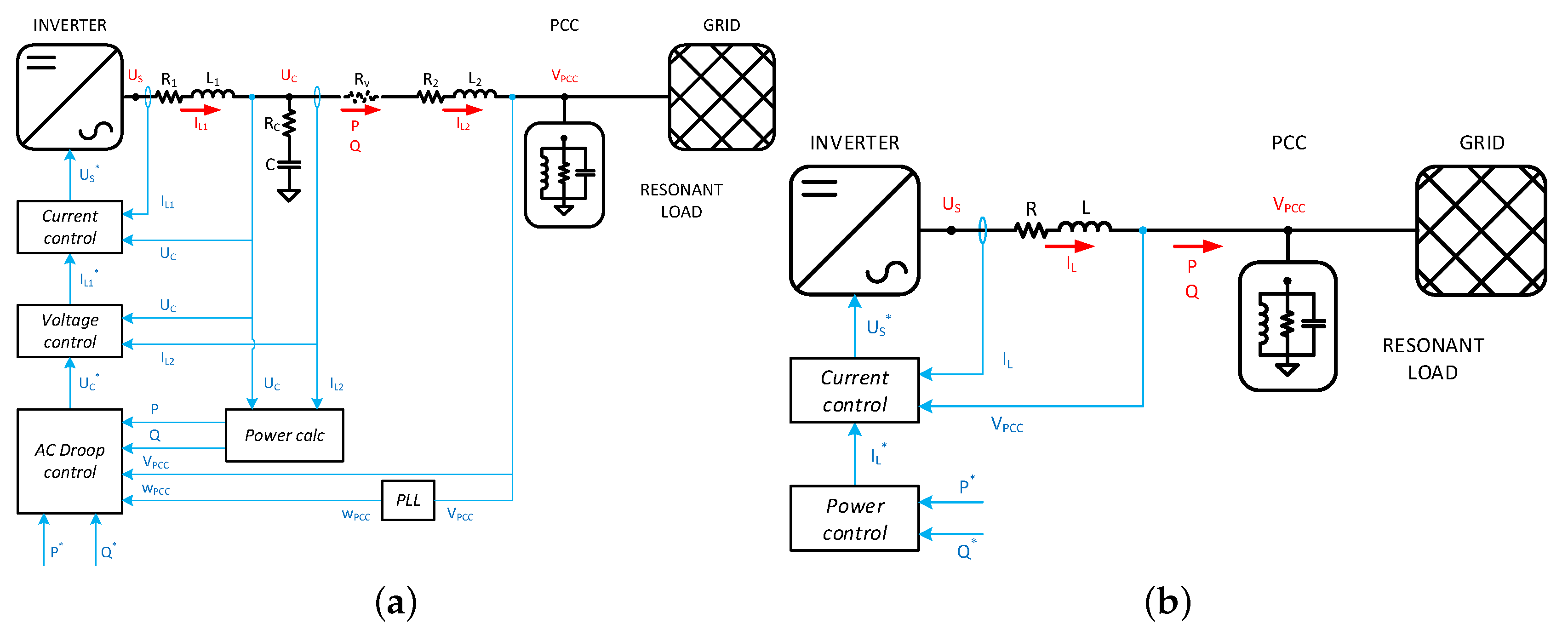
A VC-VSI requires, at least, disposing of an LC-type (inductive-capacitive) filter at its output; see Figure 1a. The AC capacitor voltage, $U_C$, is managed by a voltage control loop. Its control action regulates the reference of the inner current loop, $I_{L_1}^{*}$, ensuring the converter current during operation. Usually, a second inductance is also considered, $L_2$, which represents the aggregation of the leakage inductance of a transformer and the line impedance between the capacitor and the point of common coupling (PCC). This impedance makes possible a third master control loop corresponding to the AC droop control in GSCI. This allows handling the power exchange with the mains. Its control action determines the amplitude and phase for the voltage reference $U_C^{*}$. Accordingly, the aim of using an AC droop control strategy is to allow the operation of several VC-VSI in parallel, mainly without the use of communications [8,9,10]. AC droop control is usually considered as a non-ideal voltage source because its apparent power regulation is achieved by managing the difference of the frequency and voltage amplitude between $U_C$ and $U_{PCC}$.

On the other hand, a CC-VSI only strictly requires an inductive output filter. Apparent power can also be controlled, but it is directly regulated according to a translation from the apparent power reference to amplitude and phase in terms of current, as shown in Figure 1b. The active or reactive power amount can be simply translated to current by the ratio of the reference over the instant voltage or the instantaneous voltage lagging a grid quarter period, respectively.

2.2. Zero Power Flow Concept

Figure 1 shows an inverter connected to the grid with the resonant load type proposed in the mentioned AI standards [7,11,12]. They suggest that the concept of resonant load take place when the local consumption is nearly equal to the active power given by the inverter in terms of current, considering no reactive power, but with a resonance between the reactive components equal to the frequency of the grid. On the one hand, the active part is modeled by a lumped resistance. On the other hand, an inductance is parallelized with a capacitance to achieve the resonance frequency.

It should be highlighted that when the load is under resonance, there is no reactive consumption. Note that the resonance concept is linked to a voltage driven from the current delivered by the inverter. This conventional resonant concept is limited and less significant for VC-VSI where the voltage at the PCC is explicitly controlled by the inverter. In other words, this is due to the voltage and frequency being maintained by the control law of the inverter. Thus, when using VC-VSIs, the voltage loop stunts the mains loss detection. Note that these situations are possible even though the PCC power flow is nonzero. When the mains are lost, the voltage of the PCC, $U_{PCC}$, is not released and becomes conditioned by the inverter. When the grid is off, the grid inertia is free, and $U_{PCC}$ becomes indirectly controlled by the inverter. As can be seen in Figure 1a, the AC capacitor voltage $U_C$ and the $U_{PCC}$ voltage are connected only through the output coupling impedance constituted by the inductance $L_2$ and its equivalent series resistance $R_2$, which are usually small in value.

According to the exposed arguments, it is appropriate to reconsider the resonant load concept. The resonant load purpose is to be the worst scenario for the AI methods based on voltage and frequency displacements (AI-PM (Passive Methods)and AI-PF (Positive Feedback)), refer to Section 3 for better understanding. Thus, the worst scenario occurs assuming the power flow through the PCC (active and passive) to be about zero [28,30]. Accordingly, the conception of zero (ZPF) or non-zero power flow (NZPF) exposed points out the resonant condition.

3. Main Anti-Islanding Detection Methods

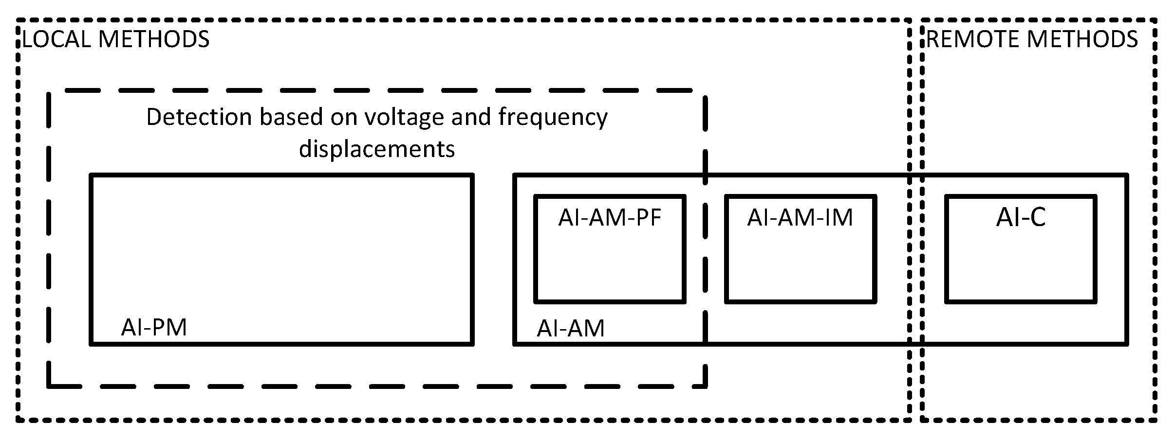
Anti-islanding detection methods (AIDM) have been evolving during the last few decades. A summary picture of the main AIDM can be seen in Figure 2, in which two categories can be defined: local or remote, according to if the AIDM is or is not part of the inverter itself. Then, three sub-categories can be considered; passive methods (PM), active methods (AM), and methods based on communications (C).

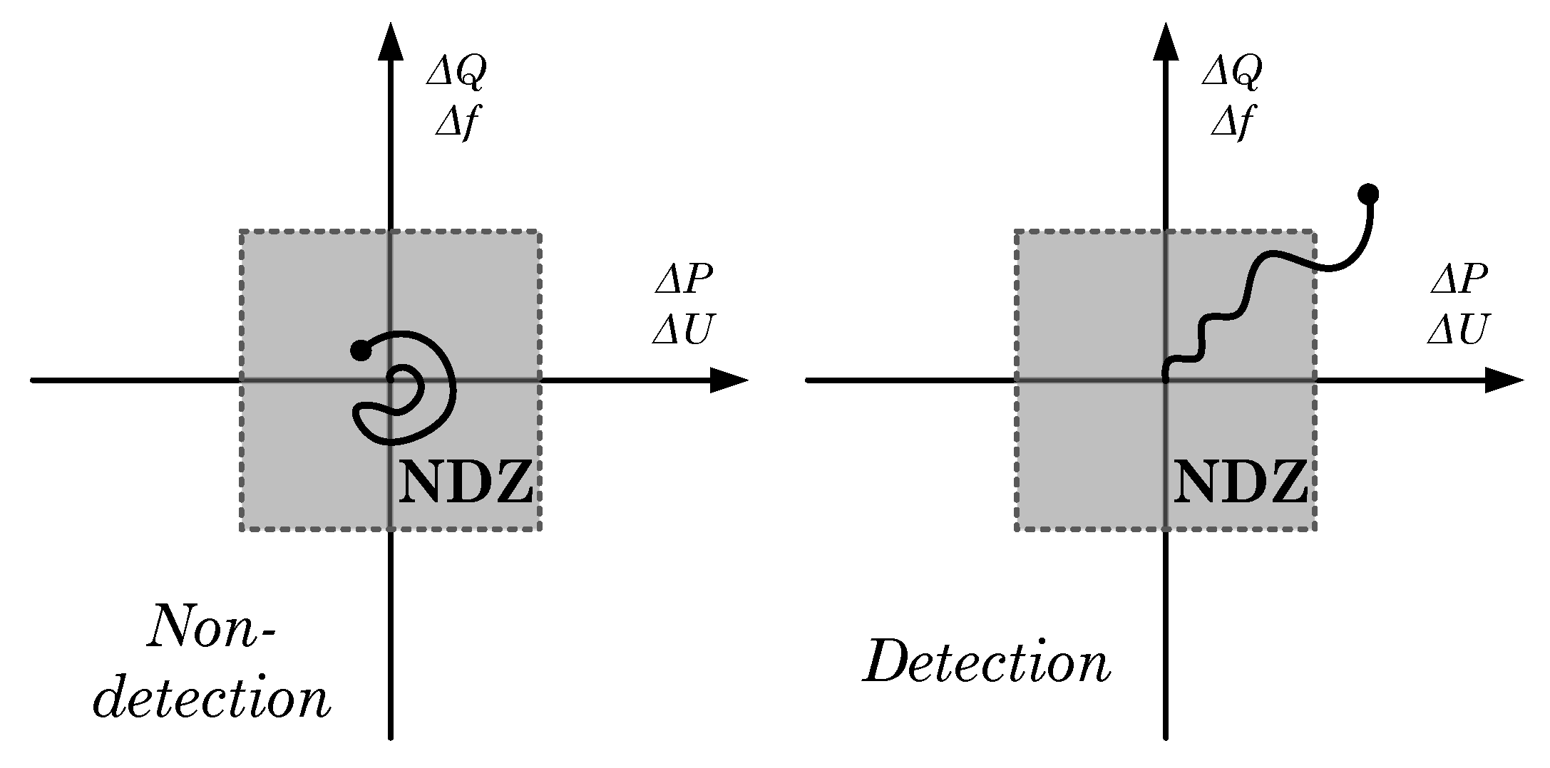
The first adopted solution, called passive methods (PM), is based on the observation of the point of common coupling (PCC) (refer to Figure 1) to detect the loss of mains by means of monitoring the voltage or the frequency variations [31,32,33]. Passive detection methods (PM) operate by monitoring the voltage amplitude and the frequency of the PCC defining a non-detection zone (NDZ). The NDZ is essentially a window defined by the voltage amplitude and frequency thresholds where the inverter is not able to detect any island event. When the mains are off, due to any external occurrence (intentional or non-intentional), the voltage or the frequency could be pushed enough to exceed NDZ limits, as is described in Figure 3.

However, if a local load, usually called resonant load, is consuming all the power (active and reactive) that the inverter is delivering when the utility goes off, neither the voltage nor the frequency will change significantly. This fact hinders the island detection. Thus, active methods (AM) appeared to overcome this challenge. Their aim is to observe, as well as to provoke a perturbation, boosting the variation of some electric variable, consequently enhancing that observation. According to their operating principle, they can be classified into three main groups:

-

Positive feedback (PF): These are active methods injecting some perturbation in order to generate a voltage or frequency drift to make evident the islanding transition. Several examples can be found in the literature: active frequency drift (AFD) [31,32], slip mode frequency shift (SMS) [31,32,33,34], Sandia voltage shift (SVS), and Sandia frequency shift (SFS) [31,32,35].

-

Impedance measurement (IM): An impedance measurement mechanism detects the utility disconnection thanks to the impedance change of the PCC. Some authors started using external switching impedances devices [36,37], but the increase of the computational capabilities of the inverters microcontrollers makes them able to inject harmonics under different approaches: simple harmonic injection [31,38], double harmonic injection [31,38], and also using inter-harmonics [39,40,41]. Finally, as indirect harmonic injection, PLL (phase locked loop) can also be found [29,31], as well as system identification-based methods [42].

-

Based on communications [25,26]: Some signal generator based on different carrying means aims to provide the state signals of the mains. Some examples of such possibilities are radio, power line carrier communication, power signals, or wireless alternatives. They usually need a remotely located transmitter and receiver, and this responds to why it is considered a remote AIDM. However, it is possible to find some examples based on a power device itself under a local conceptualization [25].

4. Limitations of AIDMs When Applied with the Presence of GSCI

This section aims to expose the limited capacities or constraints from those AI-PM and AI-AM locally embedded in a GSCI. AI-C are out of the scope of the present paper because they usually imply remote requirements. Thus, this section leads to answering why the AI-IM method results in a proper solution and contributes to analyzing the useful frequencies to apply to it. For this purpose, the frequency detection bandwidth (DFBW) will be introduced and evaluated according to the impedance PCC transfer function.

4.1. Passive Method Type

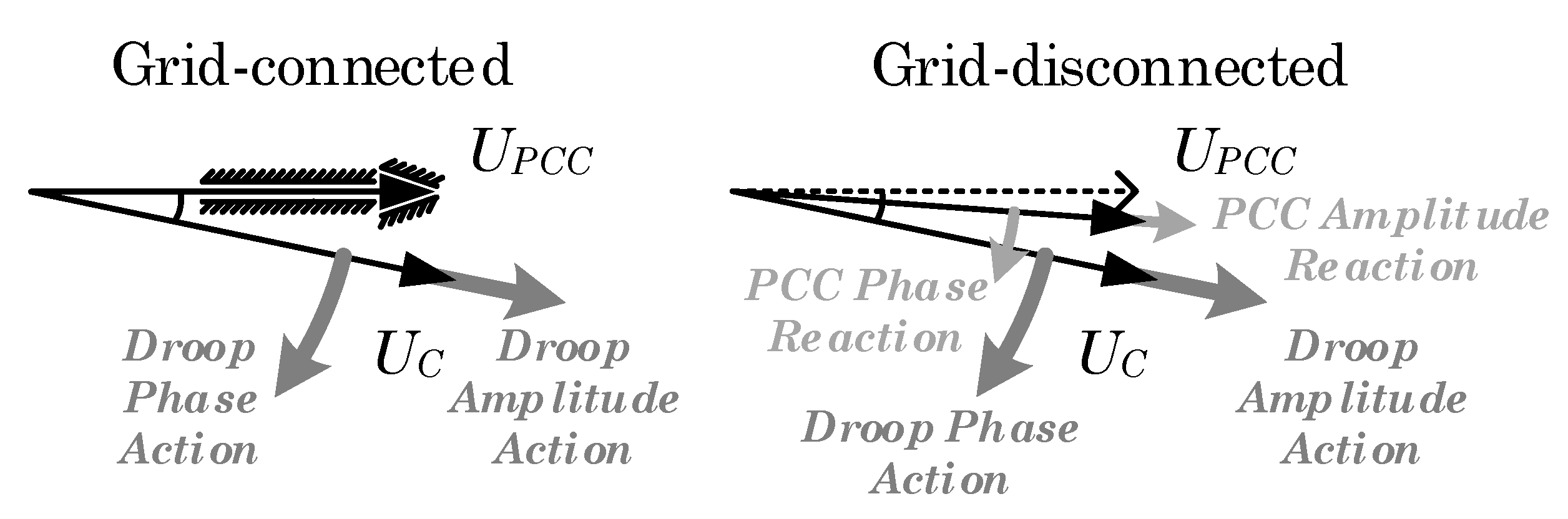
A droop control strategy is usually used in inverters (GSCI case) due to its ease of parallelization [4,5,9,10]. The droop control manages the active and reactive power, modifying the module and phase of the AC capacitor voltage $U_C$ [9,10] with respect to the PCC voltage $U_{PCC}$. Nevertheless, for its proper operation, the droop control is based on grid-connected operation and needs the grid to hold the voltage of the PCC (module and phase). Due to this, the droop control requires great effort to change the injected power, active or reactive, under the absence of the mains. In other words, when the voltage loop’s control action attempts to correct $U_C,$ so that it varies the power flow exchange with $U_{PCC}$, the $U_{PCC}$ follows $U_C,$ which results in displacement. This phenomenon is qualitatively represented in Figure 4 by a mechanical analogy. In grid-connected mode, the grid is the point of support, i.e., acts as a wall/ground surface. Thus, the phase and amplitude between $U_C$ and $U_{PCC}$ are the “forces” connected to the point of support by rotational and linear springs, respectively. These springs are related to the impedance between $U_C$ and $U_{PCC}$. The more “elongation” there is or the more “angle rotated” it is, the more the “force” results (active or reactive power managed by means of droop phase or amplitude action). In the case of grid absence, the point of support is lost, and any effort in gaining elongation or angle by $U_C$ will consequently drag $U_{PCC}$.

Although droop’s control actions are affected by the sudden power flow interruption of grid-connected to grid-disconnected transitions, the effects result in being excessively smooth. This is due to the implicit slow dynamic behavior when emulating synchronous generator inertias [5]. Thus, due to a reduced time response, as well as limited droop control action’s swing (in terms of voltage amplitude and phase), PM are not adequate because several standards require a detection in less than 160 ms, as will be detailed in Section 4.2.4. Thus, AI-PM shows an implicit lack of effectiveness in the conventional concept of resonant load and NZPF and ZPF.

4.2. Active Method-Positive Feedback Type

In order to boost the potential of island detection, AI-AM are widely used in contrast to AI-PM. In the following lines, why AM-PF characterized by voltage and frequency shifts are not adequate when ZPF is assumed in VC-VSI is detailed. Thus, the following lines put the focus on the lack of effectiveness of the main AM-PF options; slip mode shift (SMS), active frequency drift (AFD), and Sandia voltage or Sandia frequency shift (SVS or SFS).

4.2.1. Operating Principle

Any AI-AM establishes different mechanisms to perturb, at least, one of the controlled arguments of an electric magnitude. The direct consequence is an intrinsic distortion of the waveform quality. Considering that the inner controlled magnitude is the inverter’s output current, $I_{L1}$ (see Figure 1), it can be time-varying, described as:

$$i_{L1}\left(t\right)=I·sin(\omega t+\varphi )$$

(1)

Thus, according to the perturbation strategy, it is possible to change the peak amplitude of the controlled current I, the frequency $\omega$, or the phase $\varphi$. Some AM-AI methods are called PF methods because their objective is try to make unstable, by some means, the controlled magnitude. The use of the current is the option addressed more often in the literature for AM-PF [31,32,33,34,35].

When the inverter goes from grid-connected to grid-disconnected, the behavior of the voltage and frequency at the PCC is directly related to the impedance and the resonant load power consumption. In terms of the quality factor, q, and the resonant angular frequency, ${\omega }_r$, obtained as:

$$\begin{array}{c}q=R_{RL}·\sqrt{\frac{C_{RL}}{L_{RL}}}\hfill \\ {\omega }_r=\frac{1}{\sqrt{L_{RL}·C_{RL}}}\hfill \end{array}$$

(2)

the resonant load impedance and its phase can be expressed by:

$$\begin{array}{c}{\overrightarrow{Z}}_{RL}=R_{RL}·\frac{1}{1+j·q\left(\frac{\omega }{{\omega }_r}-\frac{{\omega }_r}{\omega }\right)}\hfill \\ {\theta }_{RL}=arctan\left(-q·\left(\frac{\omega }{{\omega }_r}-\frac{{\omega }_r}{\omega }\right)\right)\hfill \end{array}$$

(3)

where $R_{RL}$, $L_{RL}$, and $C_{RL}$ are the resistance, the inductance, and the capacitor that characterize the classical definition of a resonant load, respectively. Otherwise, the active, $P_{RL}$, and reactive, $Q_{RL}$, power consumption of this kind of resonant load can be expressed as:

$$P_{RL}=U_{PCC}^2·\frac{1}{R_{RL}}$$

(4)

$$Q_{RL}=U_{PCC}^2·\left(\frac{1}{\omega ·L_{RL}}-\omega ·C_{RL}\right)$$

(5)

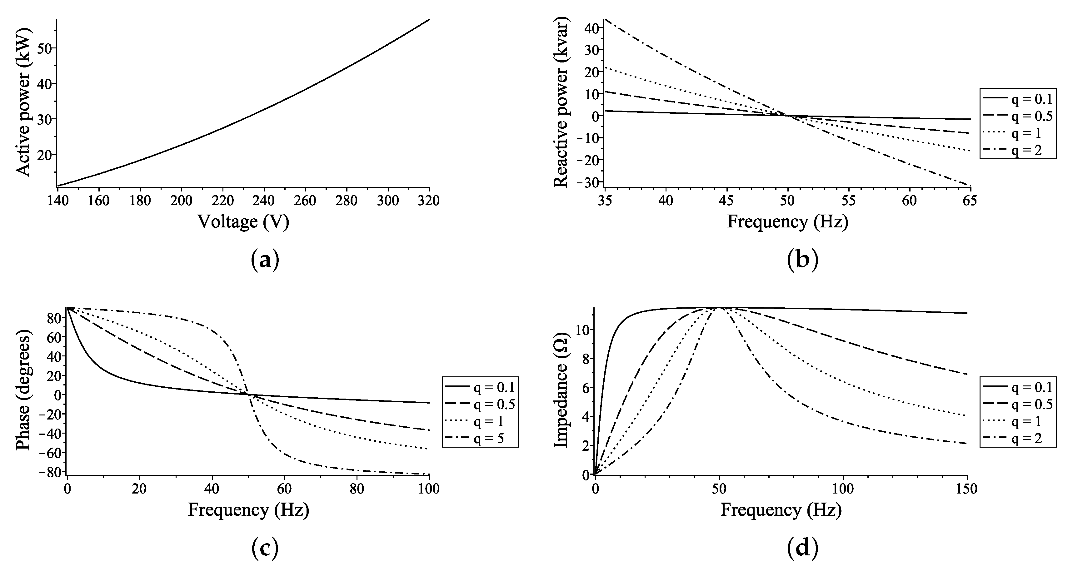
which can be represented in terms of q and ${\omega }_r$, by:

$$Q_{RL}=U_{PCC}^2·\frac{q}{R_{RL}}·\left(\frac{{\omega }_r}{\omega }-\frac{\omega }{{\omega }_r}\right)$$

(6)

Figure 5a shows the active power versus voltage and will be used as the basis plot for Figure 5b–d in which the quality factor q is considered. It can be seen in Figure 5b–d, deduced from Equations (3) and (6), that the impedance (module and phase) and the reactive power slopes close to the resonant frequency are highly sensible with the quality factor q. Thus, it is a significant effect that the quality factor q affects AI strategies based on voltage and frequency displacements. The higher the quality factor q, the bigger will be the reactive power mismatch needed to move the frequency.

Notice that when grid-disconnected, AM-PF are acting on the local load characteristics to push the PCC voltage or frequency from the NDZ.

4.2.2. Slip Mode Frequency Shift

SMS is an AM-PF that tries to destabilize the inverter by changing the frequency of the delivered current [31,32,33,34]. It is based on the phase characteristic of the conventional resonant load concept. Thus,

$${\theta }_{RL}=arctan\left[-q·\left(\frac{f}{f_r}-\frac{f_r}{f}\right)\right]$$

(7)

where ${\theta }_{RL}$ is the present phase in grid-disconnected mode absorbed by the resonant load, f is the frequency at the PCC, and $f_r$ and q are the resonant frequency and quality factor of the local resonant load, respectively. In order to make the frequency unstable, a perturbation is added on the current injected phase,

$${\theta }_{SMS}={\theta }_m·sin\left(\frac{\pi }{2}·\frac{f-f_r}{f_m-f_r}\right)$$

(8)

where ${\theta }_{SMS}$ is strictly the phase of the set-point current and ${\theta }_m$ and $f_m$ are the SMS parameters.

From Equations (7) and (8), it can be deduced that when grid-connected, the utility holds the frequency about its fundamental value [31]. Even so, when grid-disconnected, this is an unstable equilibrium point, and the frequency is forced to move out from the NDZ. However, SMS has to be injected by means of current directly to the resonant load, taking into account that the outermost controlled variable is $U_C$. This AM results in being meaningless for GSCI.

4.2.3. Active Frequency Drift

AFD is a PF method that shares the same aim as SMS [31,32]. The inverter current is distorted with a small zero current segment. Then, the current trends to change the frequency held by the grid. However when grid-disconnected, the frequency is drifted away from the NDZ. Once again, as like SMS, AFD has to be injected by means of current directly to the resonant load, and it is useless for VC-VSI.

4.2.4. Sandia Voltage Shift and Sandia Frequency Shift

SVS and SFS are two important AM based on PF strategies [31,32,35]. As a difference from SMS and AFD, the used perturbations in these cases are not directly based on current. Derived from Equations (4) and (5), these methods aim to destabilize the voltage or the frequency by modifying the active or reactive power loops. For the following explanation, consider Figure 1a.

In the SVS case, the variation between the PCC voltage, $U_{PCC}$, and the rated voltage, $U_N$, is accumulated to the active power reference amplified by a gain factor, $k_U$, as is shown in Figure 6a. $G_{PU}\left(s\right)$ represents the transfer function, including the inverter, between the active power error and $U_{PCC}$ amplitude. If the grid is connected, the voltage variation is limited and small, offering a null average value ($\Delta P^{*}\simeq 0$). Then, it affects only slightly the power reference, $P^{*}$. If the grid is disconnected, any minor voltage discrepancy boosts (in positive or negative direction) the active power reference, which in the next algorithm iteration, will speed up $U_{PCC}$ even more.

The same idea of SVS can be exported to SFS in terms of frequency considering the negative slope of the relation between the reactive power and the frequency (refer to Figure 5b), as can be seen in Figure 6b. In this case, the amplifier factor is $k_{\omega }$, and $G_{Q\omega }\left(s\right)$ represents the transfer function, including the inverter, between the reactive power error and ${\omega }_{PCC}$.

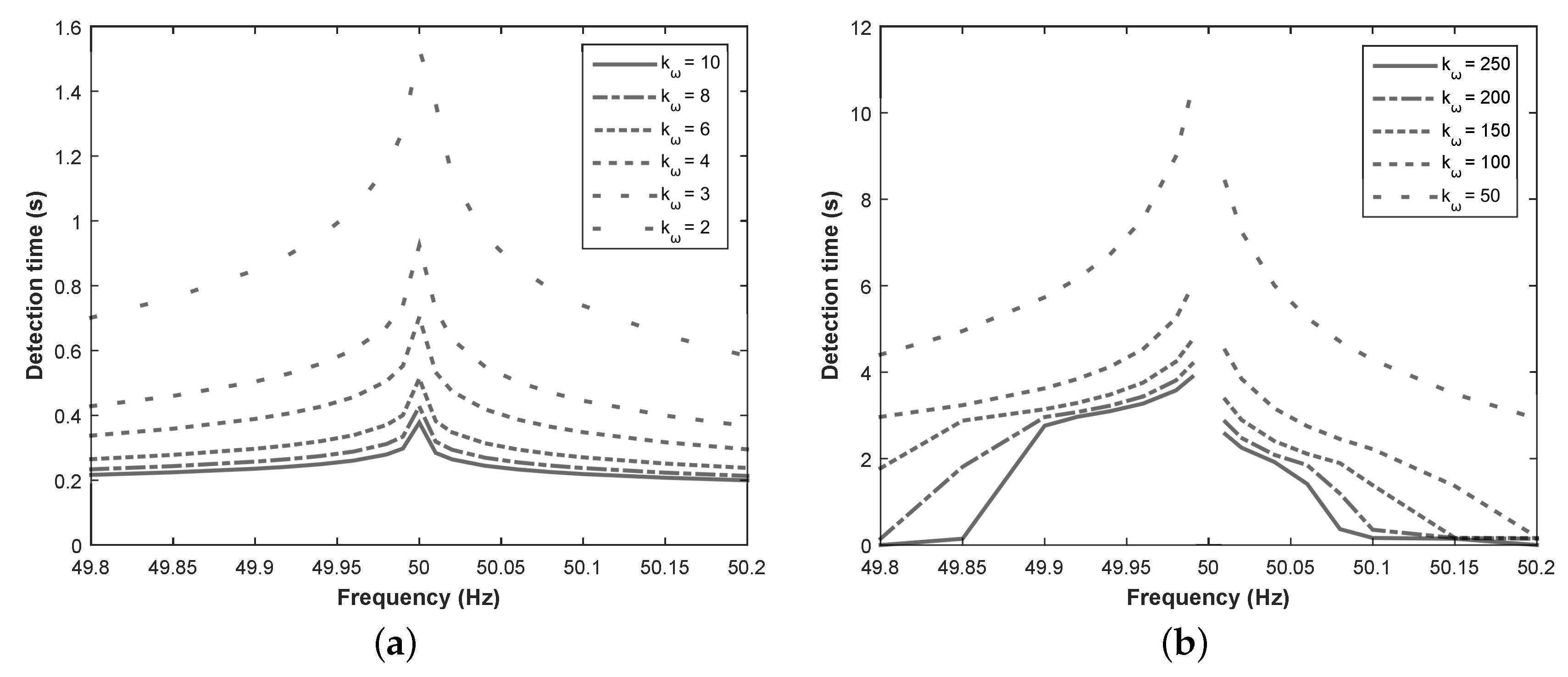
If the SFS option is simulated under a GSI or a GSCI context, it can be seen how this fact is translated to extremely high positive feedback amplifier gains. The inverter and control parameters used to evaluate this discrepancy are summarized in

Table 2. Hardware and control parameters.

LCLfilter	Output phase inductance $L_1$	250	$\mathsf{\mu }$H
	Transformer leakage inductance $L_2$	70	$\mathsf{\mu }$H
	AC capacitor C	350	$\mathsf{\mu }$F
	Switching frequency	8	kHz
Droop loop	Proportional constant for P, Q	0.00001
	Integral constant for Q	0.003
Voltage loop	PRproportional constant	0.07
	PR integral constant	0.07
Current loop	PR proportional constant	0.75
	PR integral constant	3.93
PLL loop	Settling time	5	ms

. In order to simulate CC-VSI, the voltage loop and the droop control have been removed.

Figure 7a (CC-VSI) and Figure 7b (VC-VSI) represent the detection time when the inverter delivers 30 kW. The grid to which it is connected is 230 V and 50 Hz. The resonant load is 30 kW and the quality factor $q=2$ is assumed ($R_{RL}=1.76$ $\mathsf{\Omega }$; $L_{RL}=2.8$ mH; $C_{RL}=3.6$ mF). As previously mentioned, high amplifier gains produce non-convenient disturbances. Figure 7a,b shows the islanding detection times versus the mains’ frequency at different $k_{\omega }$ factors. Figure 7a shows slow detection times as closest to the rated frequency (50 Hz in the example), which is the frequency at the PCC. This is due to the small initial error of the positive feedback loop. Even considering this behavior, the detection times results in being fast enough to achieve the proposed time in the standard. In contrast, in Figure 7b, it can be noted that the response for a VC-VSI implies higher amplifying gains to achieve acceptable detection times without guaranteeing the aforementioned threshold times. Analogous results can be obtained using SVS instead of SFS.

It can be concluded that the SVS and SFS methods reduce the NDZ, generating considerable variations in the voltage or the frequency to increase islanding detection capabilities. Nevertheless, it is essential to remark that the $k_{\omega }$ and $k_U$ factors gains are significantly higher when applied to VC-VSIs instead of CC-VSIs. The higher the $k_{\omega }$ and $k_U$ gain factors are, the higher the perturbation under grid-connected operation is required. This fact affects the quality indices of the electric magnitudes. Thus, conflicts with grid regulations can appear, meaning that maybe it is not a valid method for certified installations.

4.3. Active Method-Impedance Measurement Type

The aim of any IM active method is to determine the impedance measurement at the PCC. In order to achieve this objective, Ohm’s law can be applied, then the voltage and current values of the PCC are needed. However, the proportionality between voltage and current is only maintained if there are not any active sources participating. In this sense, to decouple the impedance value from any voltage source in the system, the voltage and current information should be obtained at a different frequency from the grid-rated one. Thus, a little disturbance is added to produce a non-characteristic harmonic current in the grid. The same harmonic voltage value is obtained from the PCC. The key challenge is to select a suitable frequency that makes the detection feasible without exceeding the maximum total harmonic distortion level.

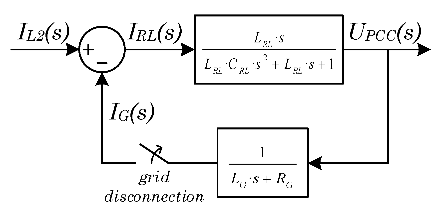
Analyzing the transfer function of the PCC impedance, the asymptotic magnitude Bode diagram for the grid-connected and grid-disconnected operation modes has been parametrized. Figure 8 represents the transfer function where the open loop block is the resonant load impedance and the feedback block is the grid equivalent series $RL$ (resistive-inductive) model admittance, both represented also in Figure 1.

The following section introduces the detection frequency bandwidth (DFBW) as a valid mechanism to explore the mentioned desired suitable frequency making IM valid and optimal.

The DFBW for IM Applicability

This paper presents a new analysis tool called DFBW that allows identifying the applicability limits of IM anti-islanding methods. The transfer function represented in Figure 8 is analyzed in detail to define the introduced concept of DFBW.

On the one hand, for the grid-connected case, the impedance Bode diagram has three characteristic angular frequencies:

-

The resonant frequency between the grid resistance and the resonant load inductance ${\omega }_1=R_G/L_{RL}$.

-

The resonant frequency between the grid resistance and inductance ${\omega }_2=R_G/L_G$.

-

The resonant frequency between the grid inductance and the resonant load capacitance ${\omega }_4=1/\sqrt{L_G·C_{RL}}$.

On the other hand, for the grid-disconnected case, the Bode diagram presents a resonance between the resonant load inductance and capacitance at ${\omega }_3=1/\sqrt{L_{RL}·C_{RL}}$.

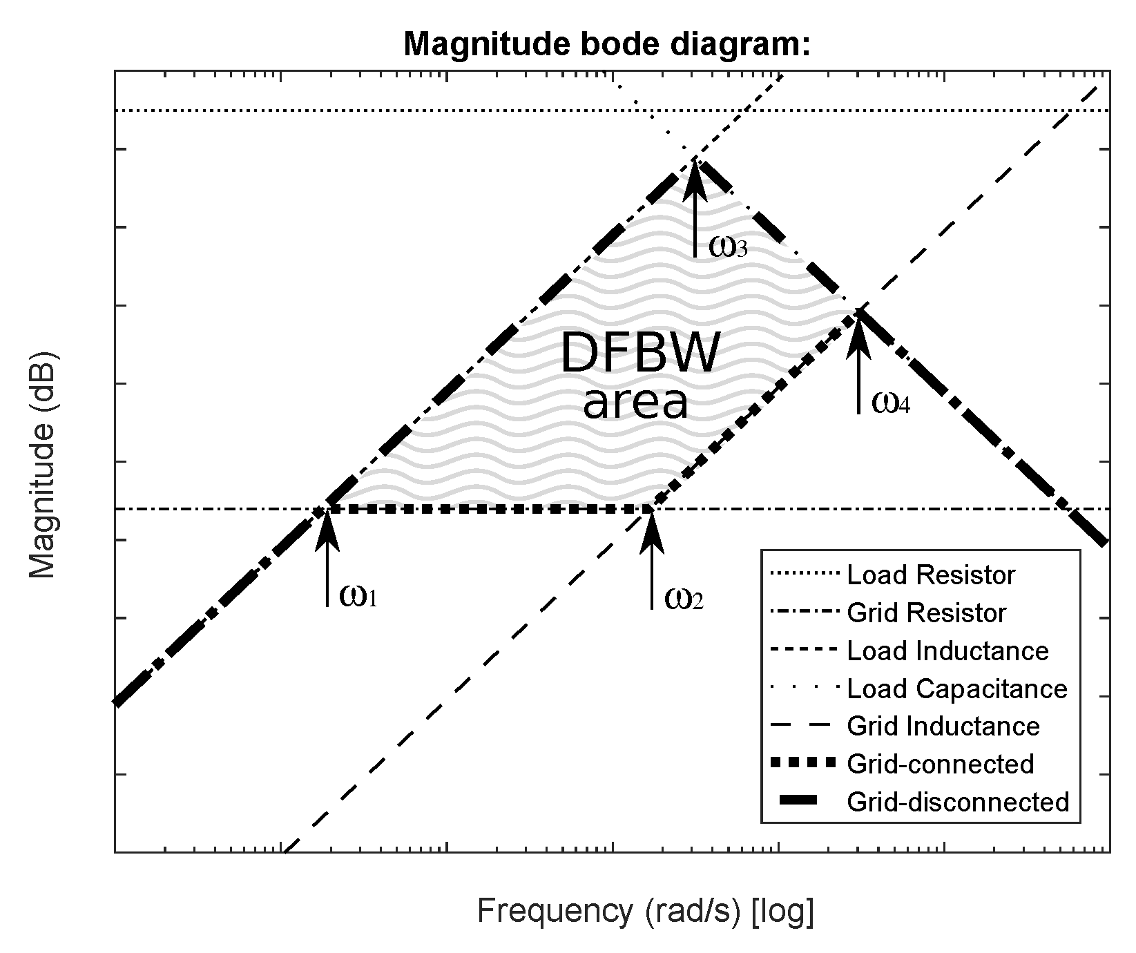
If the different asymptotes of the transfer function depicted in Figure 8 are drawn, considering ${\omega }_1$–${\omega }_4$, the area between the grid and the local load impedance Bode diagram allows defining a DFBW, as shown in Figure 9. This is a bandwidth that goes from the resonance between the grid resistance and the local load inductance ${\omega }_1$ to the resonance between the grid inductance and the local load capacitance ${\omega }_4$, and it can be expressed as:

$$DFBW=\frac{L_{RL}}{R_G·\sqrt{L_G·C_{RL}}}$$

(9)

where $R_G$ and $L_G$ are the resistance and the inductance of the grid.

Nevertheless, harmonic injection is usually used in an IM. Hence, the useful bandwidth loses the sub-harmonics area and starts on the local load resonance, which matches with the fundamental grid frequency ${\omega }_3$. Then, it is possible to redefine a new DFBW as:

$$DFB{W}^{\prime }=\sqrt{\frac{L_{RL}}{L_G}}$$

(10)

The asymptotes shown in Figure 9 are directly related to the weakness of the grid and to the quality factor q of the resonant load. Figure 10 and Figure 11 illustrate this behavior. In order to facilitate the analysis of how the asymptotes are shifted, a resonant load set at $R_{RL}=$ 1.76 $\mathsf{\Omega }$, $C_{RL}=$ 1.8 mF, and $L_{RL}=$ 5.6 mH will be considered, i.e., a 30-kW/phase resonant load. For the strong grid case, it is assumed $L_G=$ 30 mH and $R_G=$ 5 m$\mathsf{\Omega }$, while for the weak grid case, $L_G=$ 300 mH and $R_G=$ 50 m$\mathsf{\Omega }$ are taken into account.

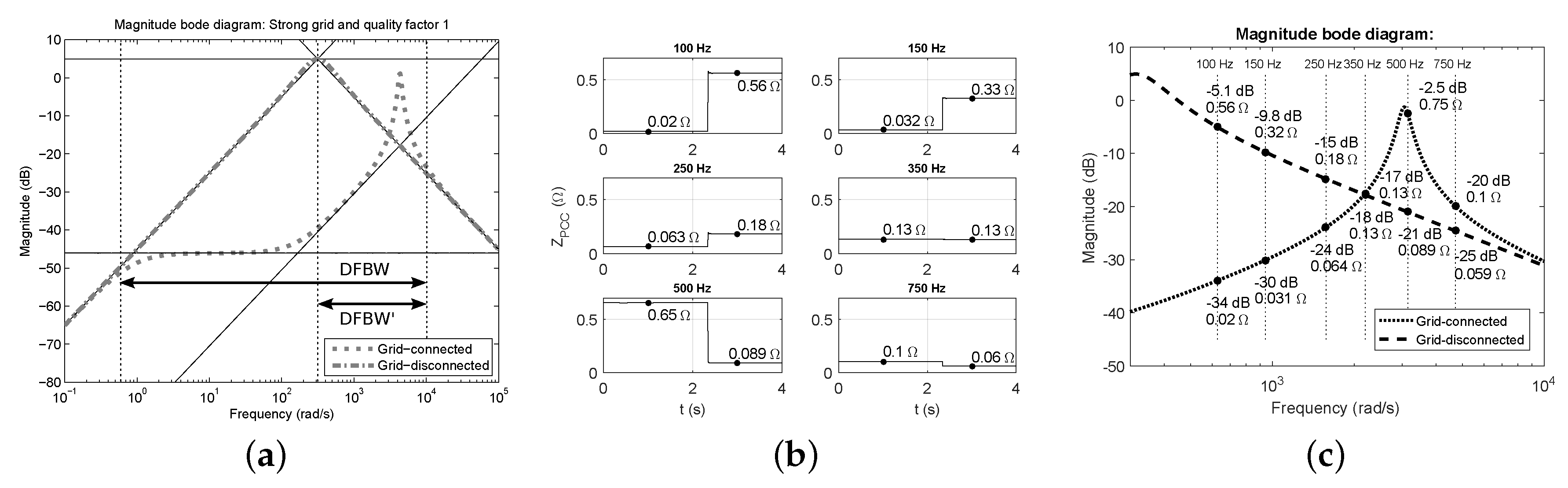
Figure 10a shows the Bode diagrams of Figure 8 for both connected and disconnected scenarios assuming the mentioned 30-kW/phase resonant load, the strong grid case, and a quality factor q set to one (the value suggested in [7,11,12]). It can be observed that the most sensitive change is near ${\omega }_3$ (314.16 rad/s for the applied case). This responds to the assumed fundamental grid frequency in the paper. Around the utility angular frequency, it is expected that the grid-disconnected impedance will be higher than the grid-connected one in terms of gain. For higher frequencies, the detection could be unattainable. This is demonstrated in Figure 10b,c, where it can be seen how the PCC impedance does not change at 350 Hz (≈2200 rad/s). This example allows deducing that the optimal multiple of the rated frequency for detection is 100 Hz (628.32 rad/s).

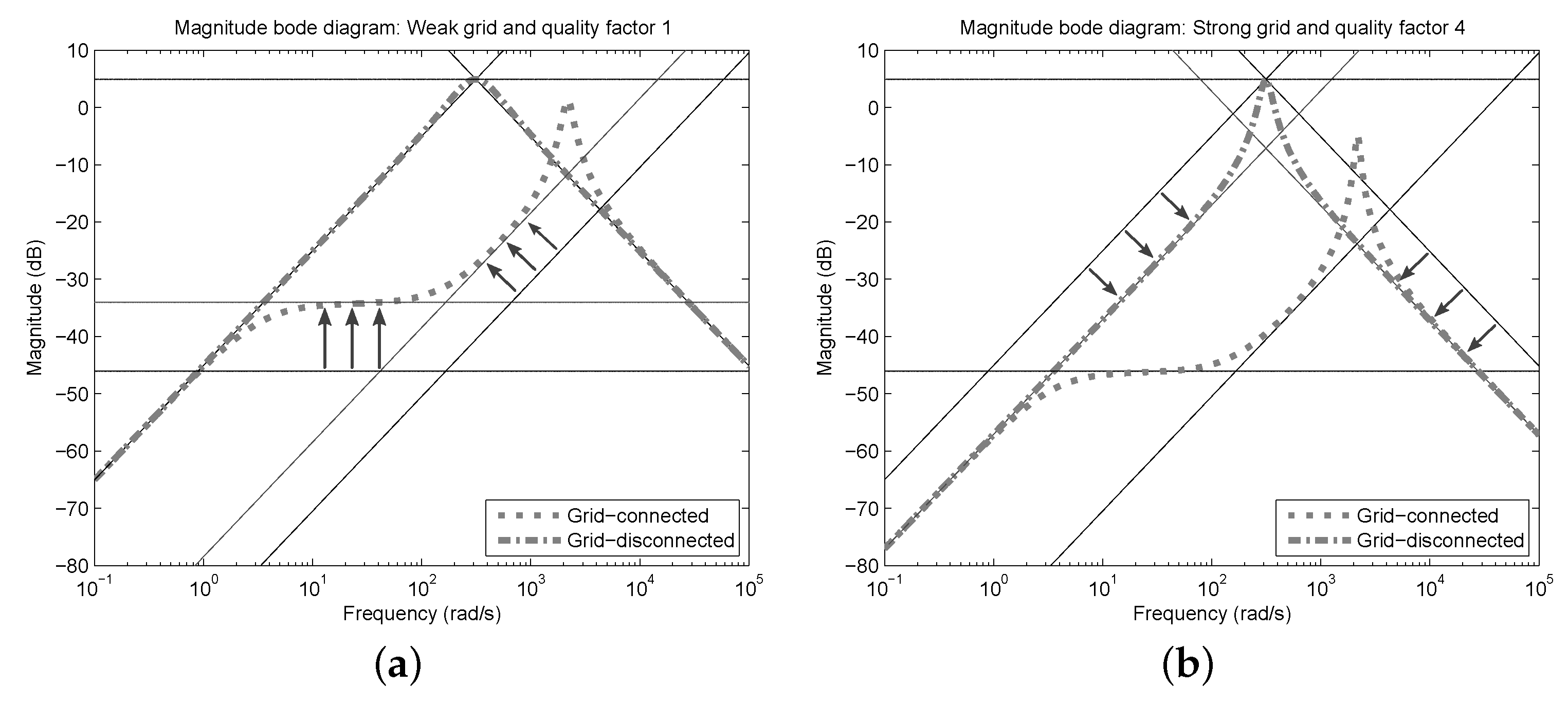
In addition, it should be noted that the DFBW not only evolves with the weakness or strength of the mains, but also with q. As can be observed in Figure 11a, the DFBW is reduced for weak grids. This is due to the vertical displacement (upwards) of the grid resistance asymptote and the horizontal displacement (towards the left) of the grid inductance asymptote. Besides, considering Figure 11b, it can seen that the higher the resonant load quality factor, the narrower the DFBW. This is because of displacement towards the right of the load inductance asymptote and towards the left shift of the load capacitor asymptote.

4.4. Partial Conclusions

As a conclusion of this section,

Table 3. Anti-islanding detection method (AIDM) versus grid support and constitution inverter (GSCI) interactions.

AIDM Category	AIDM Type	GSCI Interactions Issues	Valid?
Passive method (PM)	Voltage (V) Frequency (f)	V and f indirectly controlled by the inverter	×
Active method-positive feedback (AM-PF)	Slip mode frequency shift (SMS) Active frequency drift (AFD)	Must be implemented in current	×
	Sandia voltage shift (SVS) Sandia frequency shift (SFS)	Too slow and not suitable proportional gains	×
Active method-impedance measurement (AM-IM)	Low frequency	Out of detection frequency bandwidth (DFBW)	×
	High frequency	Islanding detection feasible	ok

summarizes per each previously-explored algorithm if it is valid as AIDM for GSCI and details the possible interactions with this inverter type. Note that even in the case of using an AM-IM as AIDM, it is not always valid and is highly dependent on the type of grid, the resonant load quality factor, and mainly, on the frequency used for the detection.

5. Improved Performance of Harmonic Injection by the Phase Perturbation Method

The AI method suggested in this paper is based on a combination of some existing solutions [29,38,39], which have been selected and adapted to fit in an experimental platform with low availability of computational time. 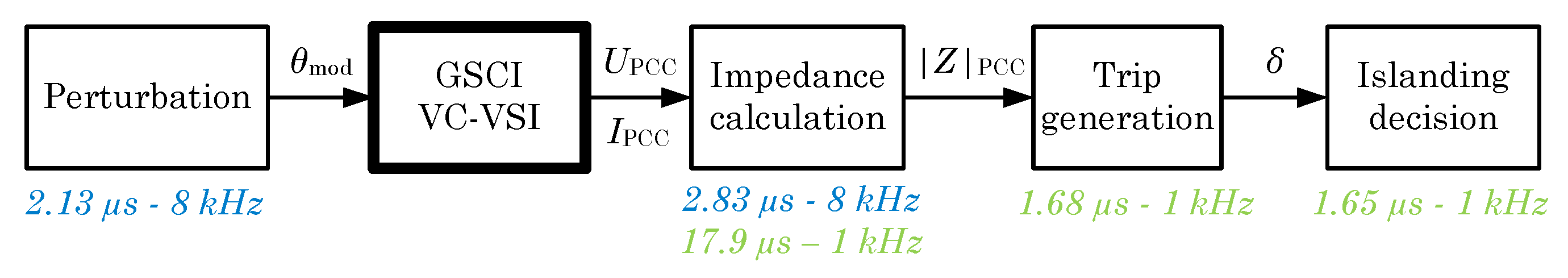These high computational requirements are typical in the case of GSCI due to the extra control needs (more control loops) and extra secondary/tertiary loops to enhance droop control [4,5,9,10]. This situation makes it especially important not to overload the inverter source code with excessive computational burden to add an AIDM. The method, presented in Figure 12, is based on different steps classified into sections for better understanding.

It should be remarked that the main idea of the proposal is to detect a change in terms of impedance, and not to be accurate in the exact value of the PCC impedance. Thus, the improvement is aligned with reducing computation burden and sharing calculations at different rates.

5.1. The Perturbation Injection (Section A)

As has been demonstrated in Section 4.3, the proper frequency for a 50-Hz rated grid is close to 100 Hz. Based on the method explained in [29], the phase reference of the voltage on the AC capacitor ${U_C}^{*}$ to inject a 100-Hz disturbance can be described by:

$${{\theta }_{mod}}^{*}={\theta }^{*}+k·cos{\theta }^{*}$$

(11)

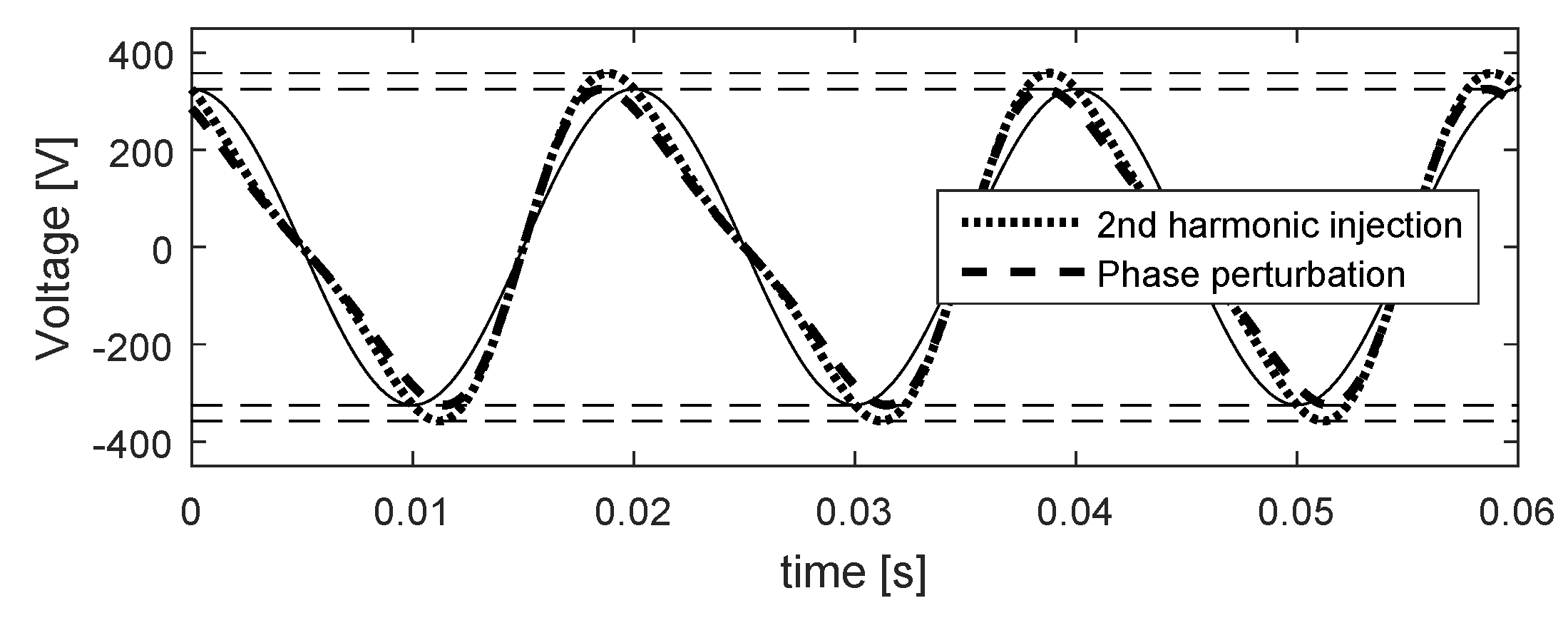
where k is an amplifying gain of the disturbance and ${\theta }^{*}$ is the phase of the referenced voltage given by the droop control. In [29], it is demonstrated that the consequence of adding this perturbation corresponds to a second harmonic injection, but without changing the zero crossing position and keeping the maximum and minimum values as the original sinusoidal waveform, as has been magnified in Figure 13. It should be highlighted that this perturbation method requires a sum, a product, and a cosine. However, the cosine argument is directly ${\theta }^{*}$ and avoids the inner product (2·$\pi$·${\omega }_r$), where ${\omega }_r$ is the rated angular frequency of the grid.

5.2. Impedance Calculation (Section B)

In [29], the island detection method is based on variations of the quadrature synchronous reference voltage considering a symmetrical and balanced system. The methodology presented in this paper is able to detect the island in a generic unbalanced system, as in [38,39], where the detection is based on impedance measurement.

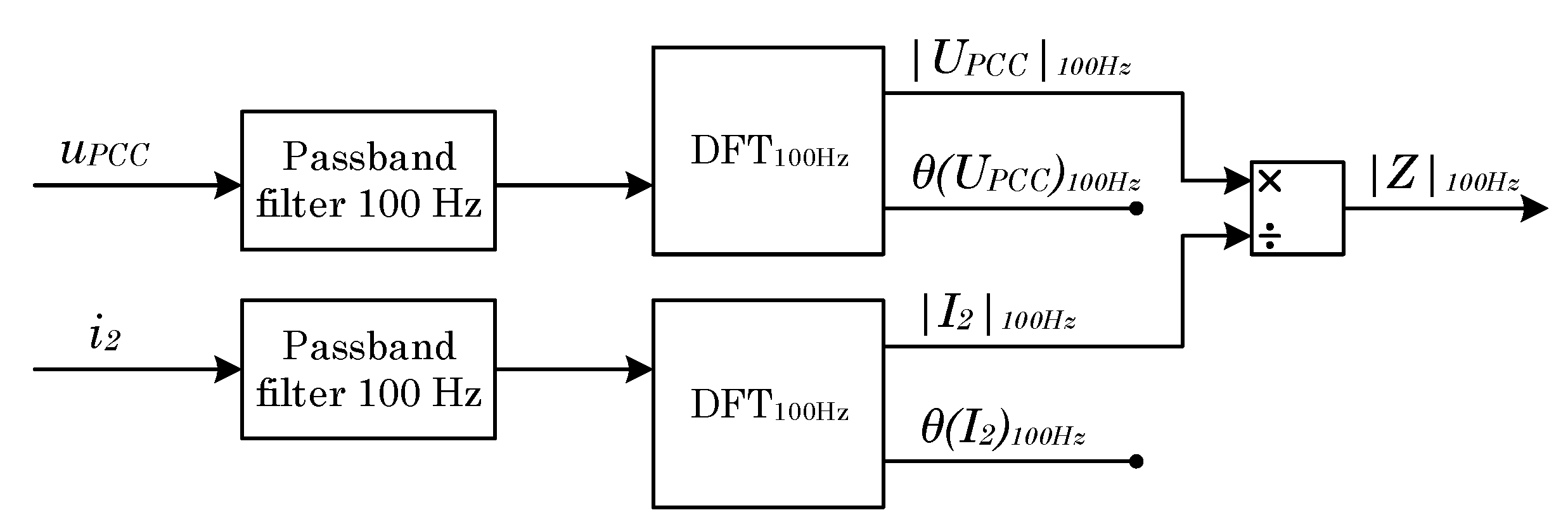
In the case of a four-wire microgrid inverter intended to operate with different power references per phase, an individual voltage measurement of each phase is needed, i.e., three degrees of freedom are being considered. Consequently, the voltage and current 100-Hz amplitude per phase must be obtained. As shown in Figure 14, the discrete Fourier transform (DTF) is used. In this case, a DFT is a mathematics calculation that requires high computational burden. However, this is implicit in any IM-based AIDM. As AIDM, the IM does not require being accurate in value, but it should be precise in value change. Thus, it is proposed in Section 5.5 to calculate the DFT at a lower frequency than that used for control purposes.

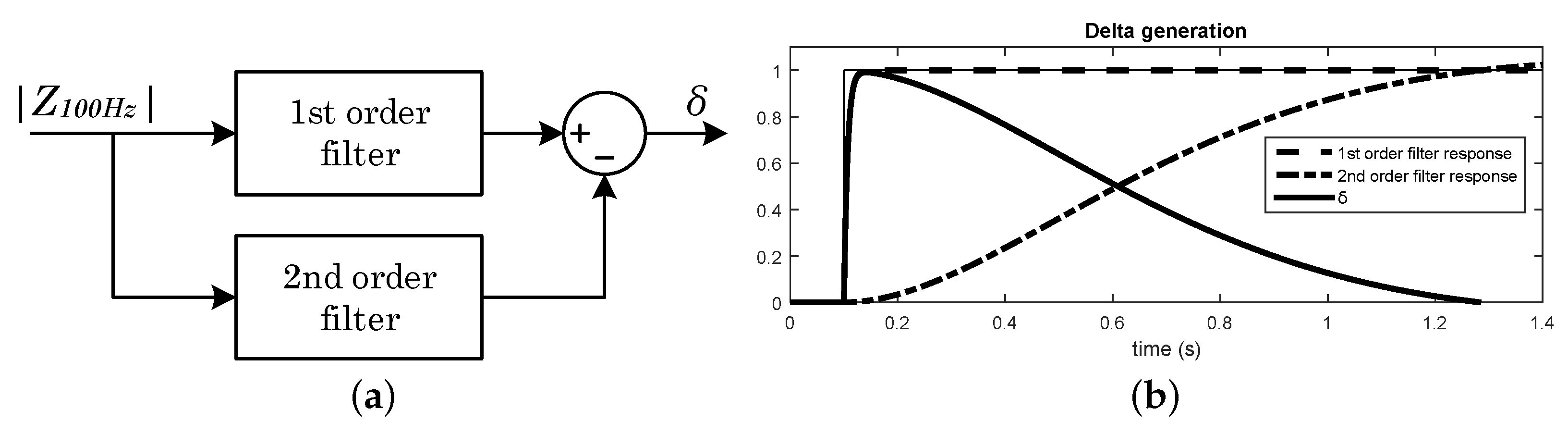
5.3. Trip Generation (Section C)

Sections A and B are intended to obtain an impedance value at PCC. The accurate value of the impedance itself is not the aim of the strategy. For this reason, the present section looks for creating a trigger signal indicating that a change in the impedance has occurred. To do this, a $\delta$ pulse will be created. This $\delta$ pulse contains the information of a grid-connected to grid-disconnected transition. The $\delta$ signal generation is obtained according to [29]. As a difference with respect to [29], instead of using a delay and average calculations, the $\delta$ pulse detection is replaced by filters; see Figure 15a. In this sense, it is possible to decrease the memory and the required computational time.

Figure 15b shows how the trip generation works. The first order low-pass filter, the faster one (about ms), intends to prevent erroneous island detections. Taking into account the time needed for the DFT, it should be set with a rising time close to the utility voltage period. Then, the second order filter, the slower one (about s), is designed to take off with a lower slope compared with the first order filter. In this sense, the $\delta$ pulse signal shows a fast rising behavior when a grid impedance change occurs and is slowly reduced to zero with a dynamics dominated by the second order filter response. Note that the $\delta$ has dynamic times in the order of the fast filter (ms).

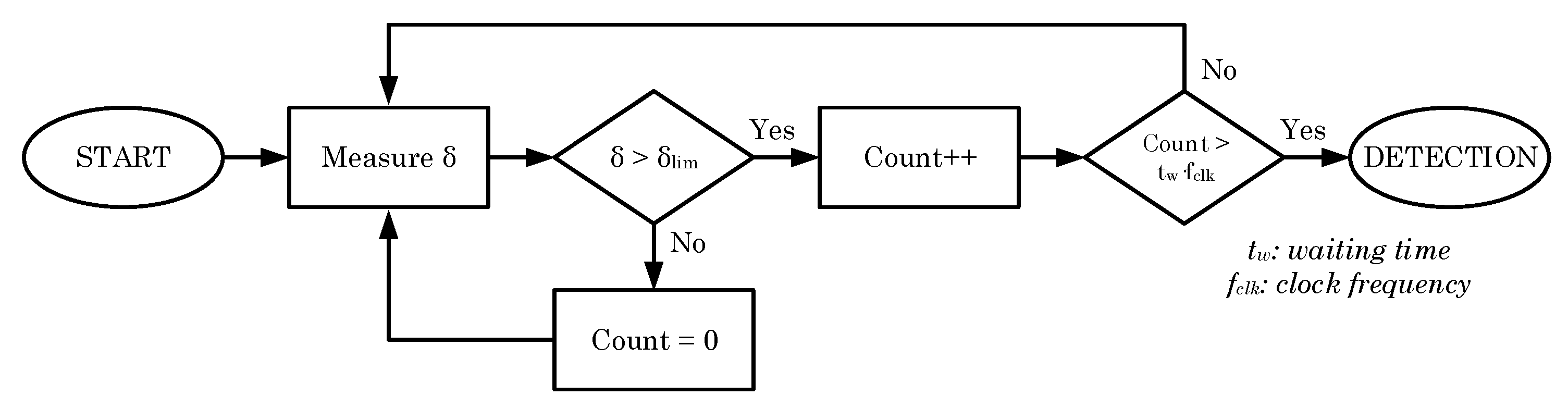
5.4. Islanding Decision (Section D)

According to all previous sections of the algorithm (A–C), at this point, it is possible to assume that the impedance at the PCC has suffered a change. However, the last step of the algorithm is presented in Figure 16 to provide a more stable decision to the islanding episode. Thus, a potential true/false grid failure flag is generated.

This final step takes the $\delta$ value from the output of Section C and contrasts it with a ${\delta }_{lim}$. The ${\delta }_{lim}$ is tuned considering the perturbation frequency and the expected DFBW. When $\delta$ exceeds ${\delta }_{lim}$, a counter allows shifting in time the decision to ensure a real detection.

Using an IM anti-islanding strategy, different from a PF one, the detection time is not directly proportional to the injected perturbation. The bigger the perturbation is, the more reliable the impedance measurement becomes, not the faster. In fact, the detection time is only fixed by the gap needed for the DFT calculation and the arranged delay by the decision.

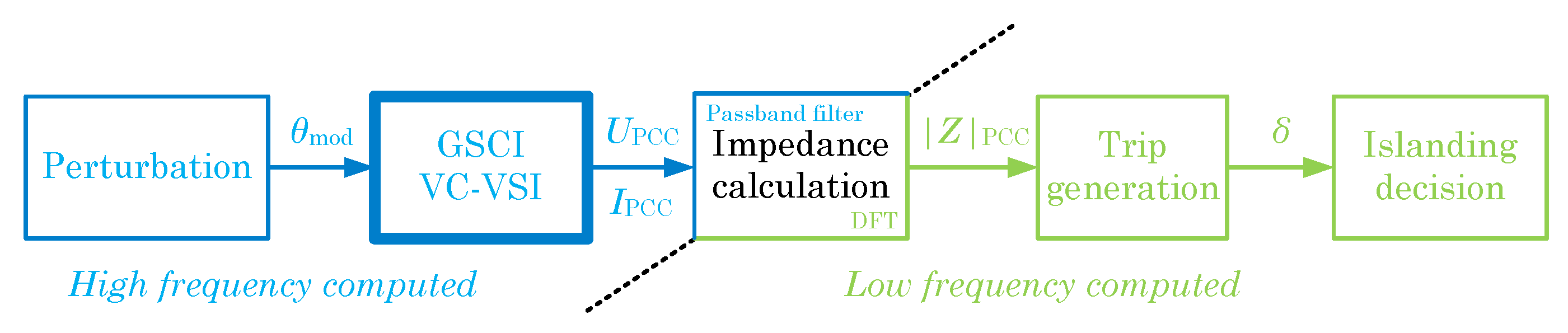
5.5. Calculation Rates Proposal

According to all previous subsections, it is proposed to apply the algorithm presented in Figure 12, but sharing the calculations at two frequency rates: one at high frequency concerning inner control loop implications and one at low frequency for the detection heavy cost functions such as the DFT, as described in Figure 17.

6. Experimental Results

This section presents the setup used for the validation of the improved IM developed in Section 5. It also evaluates the proposal in terms of cost under the setup used and the feasibility in time for the detection.

6.1. Setup

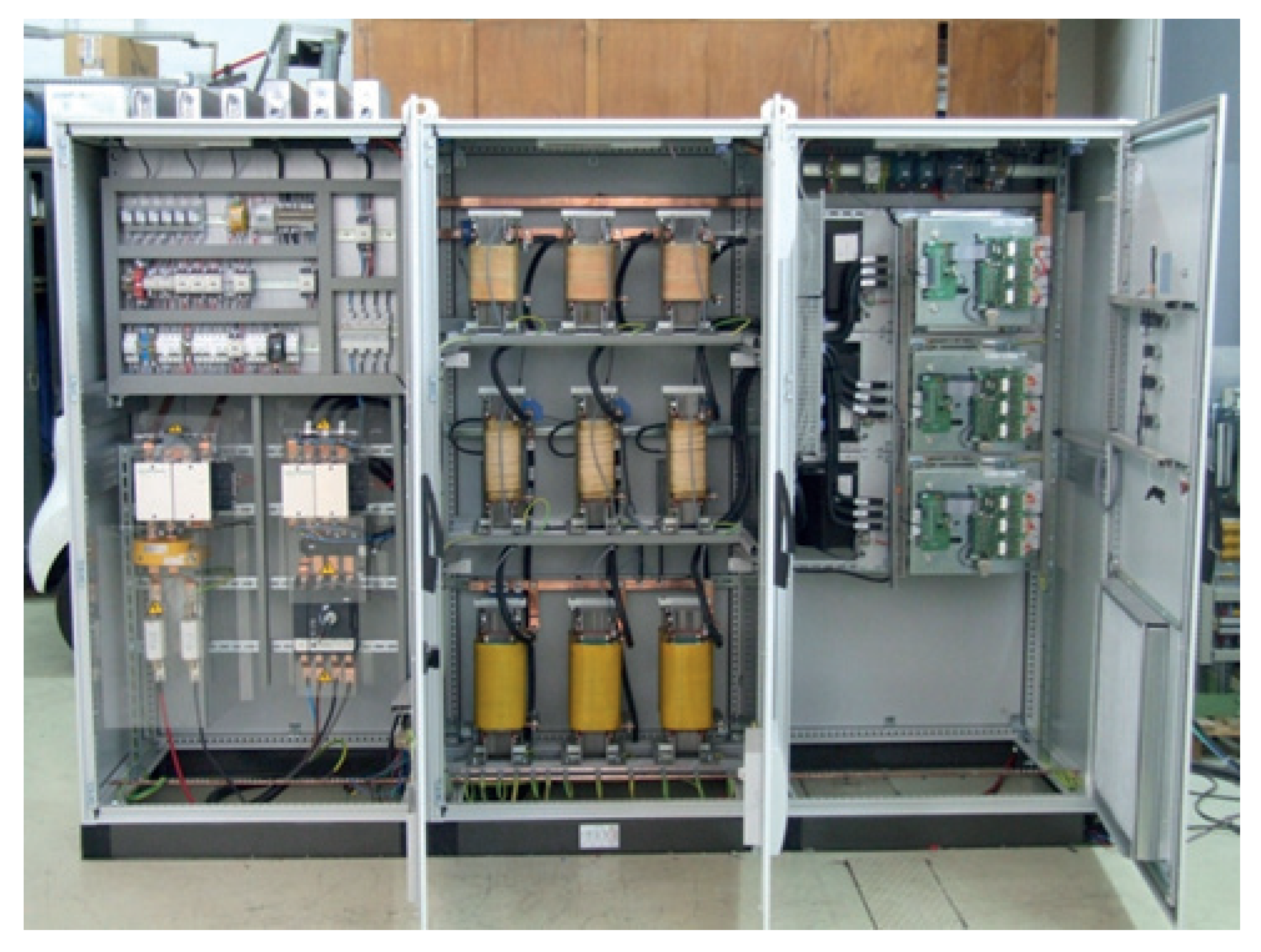
The AI algorithm has been implemented on the 90-kVA VC-VSI inverter based on three Semikron IGD-2-424 power stacks, as shown in Figure 18. The converter was a three-phase four-wire inverter, whose inner control loops (current and voltage) were based on adaptive proportional resonant controllers (PR) [30]. Each active phase was controlled independently by managing the active and reactive power set-points through an AC droop control strategy, as depicted in Figure 1a. The controller parameters and the values of the considered LCL output filter are summarized in Table 2 (same values used for simulations in Section 4.2.4).

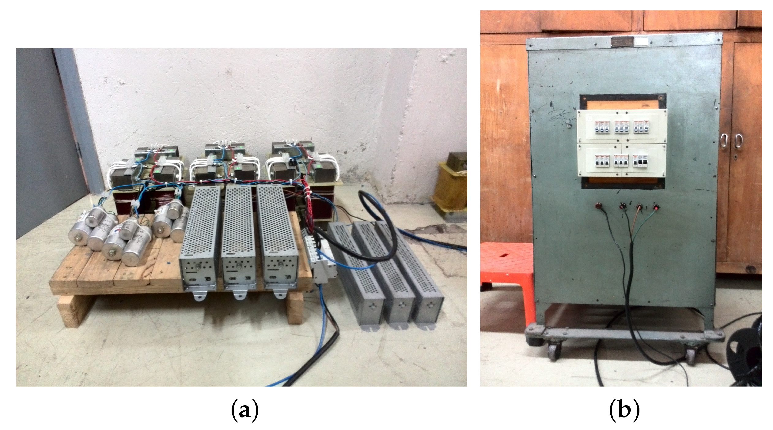
The resonant load considered was 13.8 kW (three-phase) assuming a quality factor q of 0.5 ($R_{RL}=11.5$ $\mathsf{\Omega }$; $L_{RL}=73$ mH; $C_{RL}=138$ $\mathsf{\mu }$F). In Figure 19, the experimental resonant load used is shown. As can be observed, the required physical component to achieve q at 0.5 are really bulky, requiring uncommon values of inductances, resulting in it being even more difficult to achieve q values of one or two, as requested in [7,11,12].

The detection algorithm was implemented in a TMS320F2809 DSP from Texas Instruments. The perturbation was adjusted injecting a 3.53-A${}_{rms}$ second harmonic component, which corresponds to 2.5% current harmonic distortion in grid-connected mode (when off grid, the voltage harmonic distortion was less than 2%). The islanding decision was designed to identify steps of more than 0.4 $\mathsf{\Omega }$ holding during at least 50 ms.

6.2. Results

Computational Cost

As described in Section 5.5, the calculations required to apply the proposed IM as an AIDM were split at two frequency rates. The high frequency calculations were executed every 8 kHz (125 $\mathsf{\mu }$s) and the low frequency ones at 1 kHz (1 ms). In Figure 20, the different times required to compute each section can be seen.

The total time for the high frequency calculations represented less than 4% of the available 125 $\mathsf{\mu }$s, and for the low frequency case, less than 0.5% of the available 1 ms.

6.3. Detection Validation

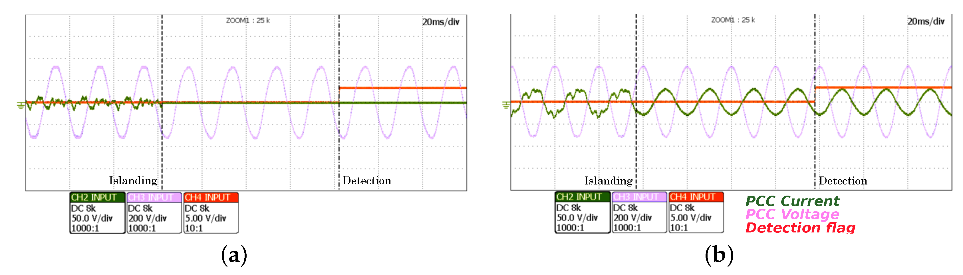
This section evaluates the detection time in the experimental setup dividing the analysis of the ZPF and NZPF scenarios.

6.3.1. Detection under Zero Power Flow

The algorithm response under ZPF conditions, where all the local loads are consuming all the generated power, can be seen in Figure 21a,b. Figure 21a refers to a detection considering that the inverter is delivering null power and there are no local loads. The detection time was achieved in 80 ms. Figure 21b presents another ZPF scenario. In this case, the inverter is delivering 4.6 kW per phase, but all this power is used to feed a local load connected at the PCC. The detection time was achieved in about 80 ms, as well.

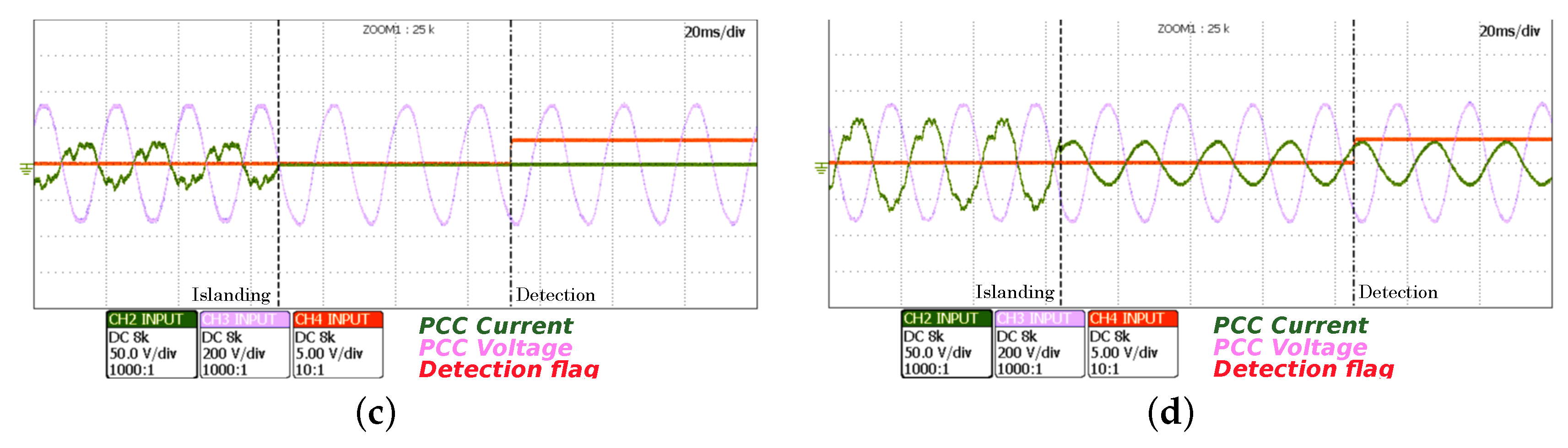
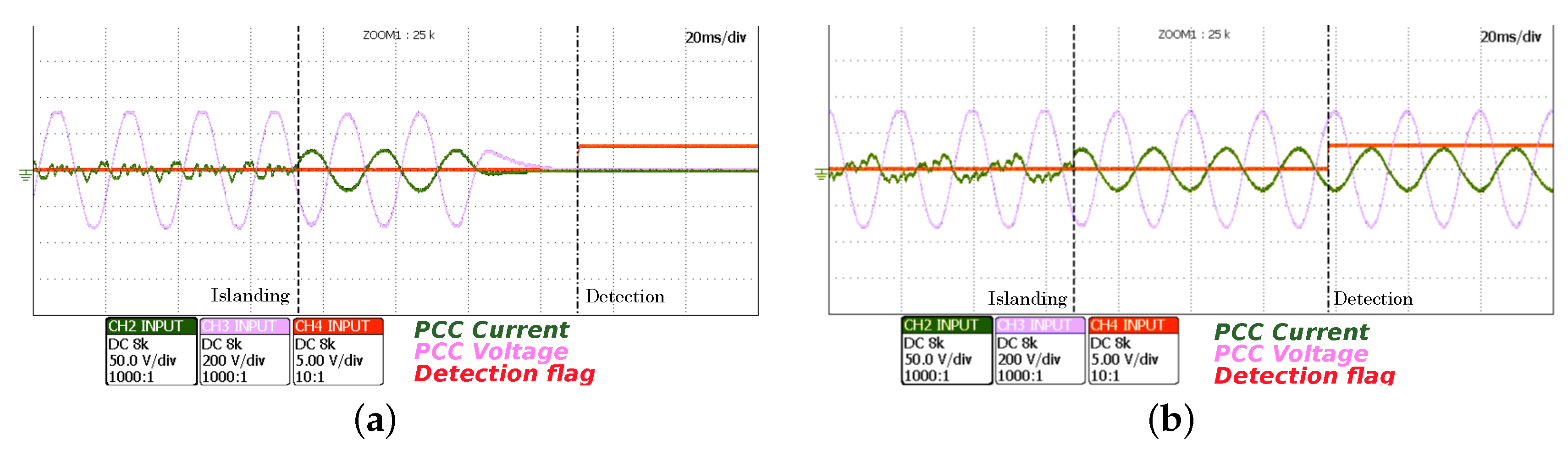
6.3.2. Detection under Non-Zero Power Flow

In the case of considering VC-VSI, both ZPF or NZPF conditions can make the island detection difficult. As has been mentioned before, this is due to the VC-VSI being the device that maintains the voltage at the PCC and not the resonant load (as is the case when CC-VSI are considered). Figure 22a–d shows the validity of the suggested AIDM also under NZPF scenarios. Figure 22a,b illustrates the detection trigger when the inverter was delivering less power than the resonant local load required. The detection times obtained were 77 and 70 ms, respectively. Finally, Figure 22c,d shows the detection trigger when the inverter exceeded the power required to feed the local load. In these last scenarios, the detections were achieved in 64 ms and 81 ms, respectively.

Note that even considering NZPF cases, the voltage magnitudes at the PCC (voltage and frequency) were practically unaltered. This is the key point of the need not to consider AIDM based on voltage or frequency displacements.

7. Conclusions

This paper presents the difference of operation applied to the anti-islanding detection methods (AIDM) when an inverter is assumed as a voltage-controlled source (VC-VSI) or current-controlled source (CC-VSI). The existence of these two types of inverters limits the conventional resonant load concept required for island detection. Thus, the concept of zero and non-zero power flow (ZPF/NZPF) was introduced to extend the worst case for island detection for either CC-VSI or VC-VSI.

The paper also clearly exposed the problem of several (passive methods, four active methods based on positive feedback strategies and impedance measurement) AIDMs operating towards VC-VSIs, especially focused on GSCIs (inverters under AC droop control strategies widely used to parallelize several units). Moreover, the effects of using AIDM methods based on voltage and frequency displacement, passive and active (positive feedback), for which the detection is not feasible, have been presented. The analysis was extended to impedance measurement (IM) AIDM, and its limitations have been detailed. This applicability limitations’ analysis was conducted to present the detection frequency bandwidth (DFBW) as a new tool that allows determining which external conditions are compatible with the detection feasibility; in other words, which kind of loads and grids (weak/strong) will be in the detection framework. In this sense, the optimal frequency to determine the impedance can be calculated.

The use of an AIDM (IM or other) in VC-VSI inverters requires a certain computational burden that usually is limited for such inverters. Thus, an improved IM method was proposed as a hybrid option based on existing methods, but focusing on the detection change and not on the impedance value accuracy. Thus, the proposed IM AIDM was split into high and low computation requirements, allowing it to be more time efficient.

The proposed IM AIDM anti-islanding method has been designed, simulated, and tested in a 90-kVA four-wire three-phase inverter. The selection of the optimal frequency to be injected for the detection method has been selected using the proposed DFBW concept. All the conducted tests have concluded that the detection strategy can be implemented with low computational costs; less than 4% for the high frequency calculations and less than 0.5% for the low frequency ones. Furthermore, the IM AIDM applied is able to generate an island detection flag below 100 ms. The detection time obtained with this method is below the minimum detection time fixed by standards of 160 ms. It is important to remark that for an IM, the consideration of a resonant load under zero power flow conditions at the PCC does not add time to the detection. Thus, for the present IM proposal, the strictest time requirements have been obtained over ZPF or NZPF situations, and CC-VSI or VC-VSI became valid, general, and efficient AIDM with a reduced computational cost.

References

- Paris: REN21 Secretariat. Renewables 2017 Global Status Report; Technical Report; REN21: Paris, France, 2017; ISBN 978-3-9818107-6-9. Available online: http://www.ren21.net/wp-content/uploads/2017/06/17-8399_GSR_2017_Full_Report_0621_Opt.pdf (accessed on 13 March 2019).
- Ramezani, M.; Li, S.; Sun, Y. Combining droop and direct current vector control for control of parallel inverters in microgrid. IET Renew. Power Gener. 2017, 11, 107–114. [Google Scholar] [CrossRef]
- Trivedi, A.; Singh, M. Repetitive Controller for VSIs in Droop-Based AC-Microgrid. IEEE Trans. Power Electron. 2017, 32, 6595–6604. [Google Scholar] [CrossRef]
- Heredero-Peris, D.; Chillón-Antón, C.; Pagès-Giménez, M.; Montesinos-Miracle, D.; Santamaría, M.; Rivas, D.; Aguado, M. An Enhancing Fault Current Limitation Hybrid Droop/V-f Control for Grid-Tied Four-Wire Inverters in AC Microgrids. Appl. Sci. 2018, 8, 1725. [Google Scholar] [CrossRef]
- De Brabandere, K. Voltage and Frequency Droop Control in Low Voltage Grids by Distributed Generators with Inverter Front-End. Ph.D. Thesis, Katholieke Universiteit Leuven, Leuven, Belgium, 2006. [Google Scholar]
- Xiao, W.; Elnosh, A.; Khadkikar, V.; Zeineldin, H. Overview of maximum power point tracking technologies for photovoltaic power systems. In Proceedings of the IECON 2011—37th Annual Conference of the IEEE Industrial Electronics Society, Melbourne, VIC, Australia, 7–10 November 2011; pp. 3900–3905. [Google Scholar] [CrossRef]
- VDE-AR-N 4105:2011-08 Power Generation Systems Connected to the Low-Voltage Distribution Network. 2011. Available online: https://www.vde-verlag.de/standards/0105029/vde-ar-n-4105-anwendungsregel-2011-08.html (accessed on 13 March 2019).
- Li, C.; Savaghebi, M.; Vasquez, J.C.; Guerrero, J.M. Multiagent based distributed control for operation cost minimization of droop controlled AC microgrid using incremental cost consensus. In Proceedings of the 2015 17th European Conference on Power Electronics and Applications, EPE-ECCE Europe 2015, Geneva, Switzerland, 8–10 September 2015. [Google Scholar] [CrossRef]
- Li, C.; Coelho, E.A.A.; Savaghebi, M.; Vasquez, J.C.; Guerrero, J.M. Active power regulation based on droop for AC microgrid. In Proceedings of the 2015 IEEE 10th International Symposium on Diagnostics for Electrical Machines, Power Electronics and Drives (SDEMPED), Guarda, Portugal, 1–4 September 2015; pp. 508–512. [Google Scholar] [CrossRef]
- Zhong, Q.; Zeng, Y. Universal Droop Control of Inverters with Different Types of Output Impedance. IEEE Access 2016, 4, 702–712. [Google Scholar] [CrossRef]
- IEEE 1547 Standard for Interconnecting Distributed Resources with Electric Power Systems; IEEE: Piscataway, NJ, USA, 2003. [CrossRef]
- IEC 61727 Photovoltaic (PV)—Characteristics of the Utility Interface. 2004. Available online: https://standards.globalspec.com/std/365170/iec-61727 (accessed on 13 March 2019).
- Ravichandran, A.; Malysz, P.; Sirouspour, S.; Emadi, A. The critical role of microgrids in transition to a smarter grid: A technical review. In Proceedings of the 2013 IEEE Transportation Electrification Conference and Expo: Components, Systems, and Power Electronics—From Technology to Business and Public Policy, ITEC 2013, Detroit, MI, USA, 16–19 June 2013. [Google Scholar] [CrossRef]
- Hossain, M.J.; Mahmud, M.A.; Pota, H.R.; Mithulananthan, N.; Bansal, R.C. Distributed control scheme to regulate power flow and minimize interactions in multiple microgrids. In Proceedings of the IEEE Power and Energy Society General Meeting, National Harbor, MD, USA, 27–31 July 2014; pp. 1–5. [Google Scholar] [CrossRef]
- Murthy Balijepalli, V.S.K.; Khaparde, S.A.; Gupta, R.P.; Pradeep, Y. SmartGrid initiatives and power market in India. In Proceedings of the IEEE PES General Meeting, PES 2010, Providence, RI, USA, 25–29 July 2010; pp. 1–7. [Google Scholar] [CrossRef]
- Yu, D.; Lian, B.; Dunn, R. Using Control Methods to Model Energy Hub Systems. In Proceedings of the Power Engineering Conference (UPEC), Cluj-Napoca, Romania, 2–5 September 2014; pp. 1–4. [Google Scholar]
- Girbau-Llistuella, F.; Rodriguez-Bernuz, J.M.; Prieto-Araujo, E.; Sumper, A. Experimental Validation of a Single Phase Intelligent Power Router. In Proceedings of the Innovative Smart Grid Technologies Conference Europe (ISGT-Europe), 2014 IEEE PES, Istanbul, Turkey, 12–15 October 2014; pp. 1–6. [Google Scholar]
- Monyei, C.G.; Fakolujo, O.A.; Bolanle, M.K. Virtual power plants: Stochastic techniques for effective costing and participation in a decentralized electricity network in Nigeria. In Proceedings of the 2nd International Conference on Emerging and Sustainable Technologies for Power and ICT in a Developing Society, IEEE NIGERCON 2013—Proceedings, Owerri, Nigeria, 14–16 November 2013; pp. 374–377. [Google Scholar] [CrossRef]
- Tirumala, R.; Mohan, N.; Henze, C. Seamless transfer of grid-connected PWM inverters between utility-interactive and stand-alone modes. In Proceedings of the APEC, Seventeenth Annual IEEE Applied Power Electronics Conference and Exposition (Cat. No. 02CH37335), Dallas, TX, USA, 10–14 March 2002; Volume 2, pp. 1081–1086. [Google Scholar] [CrossRef]
- Serban, E.; Pondiche, C.; Ordonez, M. Islanding Detection Search Sequence for Distributed Power Generators Under AC Grid Faults. IEEE Trans. Power Electron. 2015, 30, 3106–3121. [Google Scholar] [CrossRef]
- Guo, Z. A harmonic current injection control scheme for active islanding detection of grid-connected inverters. In Proceedings of the 2015 IEEE International Telecommunications Energy Conference (INTELEC), Osaka, Japan, 18–22 October 2015; pp. 1–5. [Google Scholar] [CrossRef]
- Das, P.P.; Chattopadhyay, S. A Voltage-Independent Islanding Detection Method and Low-Voltage Ride Through of a Two-Stage PV Inverter. IEEE Trans. Ind. Appl. 2018, 54, 2773–2783. [Google Scholar] [CrossRef]
- Murugesan, S.; Murali, V.; Daniel, S.A. Hybrid Analyzing Technique for Active Islanding Detection Based ond-Axis Current Injection. IEEE Syst. J. 2018, 12, 3608–3617. [Google Scholar] [CrossRef]
- Park, S.; Kwon, M.; Choi, S. Reactive Power P amp;O Anti-Islanding Method for a Grid-Connected Inverter With Critical Load. IEEE Trans. Power Electron. 2019, 34, 204–212. [Google Scholar] [CrossRef]
- Xiao, H.F.; Fang, Z.; Xu, D.; Venkatesh, B.; Singh, B. Anti-Islanding Protection Relay for Medium Voltage Feeder With Multiple Distributed Generators. IEEE Trans. Ind. Electron. 2017, 64, 7874–7885. [Google Scholar] [CrossRef]
- Pouryekta, A.; Ramachandaramurthy, V.K.; Mithulananthan, N.; Arulampalam, A. Islanding Detection and Enhancement of Microgrid Performance. IEEE Syst. J. 2018, 12, 3131–3141. [Google Scholar] [CrossRef]
- Llonch-Masachs, M.; Heredero-Peris, D.; Montesinos-Miracle, D. An anti-islanding method for voltage-controlled VSI. In Proceedings of the 2015 17th European Conference on Power Electronics and Applications (EPE’15 ECCE-Europe), Geneva, Switzerland, 8–10 September 2015; pp. 1–10. [Google Scholar] [CrossRef]
- Chillon-Anton, C.; Llonch-Masachs, M.; Heredero-Peris, D.; Pages-Gimenez, M.; Montesinos-Miracle, D. Assisting passive anti-islanding proposal for Voltage-Controlled Voltage-Source-Inverters. In Proceedings of the PCIM Europe 2018; International Exhibition and Conference for Power Electronics, Intelligent Motion, Renewable Energy and Energy Management, Nuremberg, Germany, 5–7 June 2018; pp. 1–8. [Google Scholar]
- Ciobotaru, M.; Agelidis, V.G.; Teodorescu, R.; Blaabjerg, F. Accurate and less-disturbing active antiislanding method based on pll for grid-connected converters. IEEE Trans. Power Electron. 2008, 25, 1576–1584. [Google Scholar] [CrossRef]
- Heredero-Peris, D.; Pages-Gimenez, M.; Montesinos-Miracle, D. Inverter design for four-wire microgrids. In Proceedings of the 2015 17th European Conference on Power Electronics and Applications, EPE-ECCE Europe 2015, Geneva, Switzerland, 8–10 September 2015. [Google Scholar] [CrossRef]
- Teodorescu, R.; Liserre, M.; Rodriguez, P. Grid Converters for Photovoltaic and Photovoltaic and Wind Power Systems; John Wiley & Sons, Ltd.: Hoboken, NJ, USA, 2011; ISBN 9780470057513. [Google Scholar]
- Bower, W.; Ropp, M. Evaluation of Islanding Detection Methods for Utility-Interactive Inverters in Photovoltaic Systems; Sandia Report 2002. 2002. Available online: http://www.iea-pvps.org/index.php?id=9&eID=dam_frontend_push&docID=386 (accessed on 13 March 2019).
- Singam, B.; Hui, L.Y. Assessing SMS and PJD schemes of anti-islanding with varying quality factor. In Proceedings of the First International Power and Energy Conference, (PECon 2006) Proceedings, Putra Jaya, Malaysia, 28–29 November 2006; pp. 196–201. [Google Scholar] [CrossRef]
- Liu, F.; Kang, Y.; Zhang, Y.; Duan, S.; Lin, X. Improved SMS islanding detection method for grid-connected converters. IET Renew. Power Gener. 2010, 4, 36–42. [Google Scholar] [CrossRef]
- Ye, Z.; Walling, R.; Garces, L.; Zhou, R.; Li, L.; Wang, T. Study and Development of Anti-Islanding Control for Grid-Connected Inverters; National Renewable Energy Laboratory: Lakewood, CO, USA, 2004; p. 82. [Google Scholar]
- Hopewell, P.; Jenkins, N.; Cross, A. Loss-of-mains detection for small generators. IEE Proc. Electr. Power Appl. 1996, 143, 225–230. [Google Scholar] [CrossRef]
- Kane, P.O.; Fox, B.; Mains, L.O.F. Loss of Mains Detection for Embedded Generation By System Impedance Monitoring. In Proceedings of the Sixth International Conference on Developments in Power System Protection, Nottingham, UK, 25–27 March 1997; pp. 95–98. [Google Scholar]
- Ciobotaru, M.; Teodorescu, R.; Blaabjerg, F. On-line grid impedance estimation based on harmonic injection for grid-connected PV inverter. In Proceedings of the IEEE International Symposium on Industrial Electronics, Vigo, Spain, 4–7 June 2007; pp. 2437–2442. [Google Scholar] [CrossRef]
- Asiminoaei, L.; Teodorescu, R.; Blaabjerg, F.; Borup, U. A new method of on-line grid impedance estimation for PV inverter. In Proceedings of the Nineteenth Annual IEEE Applied Power Electronics Conference and Exposition, APEC’04, Anaheim, CA, USA, 22–26 February 2004; Volume 3. [Google Scholar] [CrossRef]
- Asiminoaei, L.; Teodorescu, R.; Blaabjerg, F.; Borup, U. Implementation and test of on-Line embedded grid impedance estimation for PV-inverters. In Proceedings of the PESC Record—IEEE Annual Power Electronics Specialists Conference, Aachen, Germany, 20–25 June 2004; Volume 4, pp. 3095–3101. [Google Scholar] [CrossRef]
- Asiminoaei, L.; Teodorescu, R.; Blaabjerg, F.; Borup, U. A digital controlled PV-inverter with grid impedance estimation for ENS detection. IEEE Trans. Power Electron. 2005, 20, 1480–1490. [Google Scholar] [CrossRef]
- Liu, S.; Li, Y.; Ji, F.; Xiang, J. Islanding detection method based on system identification. IET Power Electron. 2016, 9, 2095–2102. [Google Scholar] [CrossRef]
Figure 1.
Control topology in grid-connected mode with a resonant local load. (a) Voltage-controlled voltage source inverter (VC-VSI) topology. (b) Current-controlled voltage source inverter (CC-VSI) topology. PCC, point of common coupling; PLL, phase locked loop.
Figure 2.
Anti-islanding detection methods’ classification. PM, passive methods; AM, active methods; C, communications; IM, impedance measurement; PF, positive feedback.
Figure 3.
Non-detection zone (NDZ).
Figure 4.
Vectorial representation of droop control under a grid disconnection.
Figure 5.
Resonant load characteristics. (a) Active power versus voltage of a 50-Hz resonant load. (b) Reactive power versus frequency of a 50-Hz resonant load. (c) Phase versus frequency of a 50-Hz resonant load. (d) Impedance versus frequency of a 50-Hz resonant load.
Figure 6.
AI-PF methods. (a) Sandia voltage shift (SVS). (b) Sandia frequency shift (SFS).
Figure 7.
SFS detection times applied to CC-VSI and VC-VSI. (a) Operating with a grid supply inverter (GSI) (CC-VSI). (b) Operating with a grid support and constitution inverter (GSCI) (VC-VSI).
Figure 8.
Bloc diagram of the PCC impedance transfer function.
Figure 9.
Conceptual asymptotic magnitude Bode diagram of the PCC impedance. DFBW, detection frequency bandwidth.
Figure 10.
Frequency and impedance change analysis of the PCC impedance transfer function for a strong grid scenario and 30-kW/phase with q = 1 resonant load. (a) Bode diagram (magnitude). (b) Simulations of a PCC impedance shift after a grid disconnection. (c) PCC simulation test impedances on the Bode diagram.
Figure 11.
Bode diagram of the impedance at the PCC (magnitude plot). (a) Weak grid effect. (b) q factor effect (increase value).
Figure 12.
Impedance measurement operation diagram.
Figure 13.
Magnified effect of phase perturbation distortion with .
Figure 14.
Impedance measurement diagram.
Figure 15.
Trip generation method ( pulse). (a) Generation of the signal. (b) pulse generation.
Figure 16.
Islanding decision steps.
Figure 17.
Figure 18.
Four-wire 90-kVA VC-VSI inverter.
Figure 19.
Resonant load picture. (a) Part A (inductances, capacitors, and low power resistances). (b) Part B (big resistive block).
Figure 20.
Figure 21.
Experimental results under zero power flow. (a) Null power reference zero and no local loads. (b) Inverter delivered power matching with the local resonant load consumption (4.6-kW/phase).
Figure 22.
Experimental results under non-zero power flow. (a) Zero power injection and 4.6-kW resonant load per phase. (b) Two-kilowatt power injection and 4.6-kW resonant load per phase. (c) Five-kilowatt power injection without local load. (d) Ten-kilowatt power injection and 4.6-kW resonant load per phase.