Wind Power Short-Term Prediction Based on LSTM and Discrete Wavelet Transform

Abstract

A wind power short-term forecasting method based on discrete wavelet transform and long short-term memory networks (DWT_LSTM) is proposed. The LSTM network is designed to effectively exhibit the dynamic behavior of the wind power time series. The discrete wavelet transform is introduced to decompose the non-stationary wind power time series into several components which have more stationarity and are easier to predict. Each component is dug by an independent LSTM. The forecasting results of the wind power are obtained by synthesizing the prediction values of all components. The prediction accuracy has been improved by the proposed method, which is validated by the MAE (mean absolute error), MAPE (mean absolute percentage error), and RMSE (root mean square error) of experimental results of three wind farms as the benchmarks. Wind power forecasting based on the proposed method provides an alternative way to improve the security and stability of the electric power network with the high penetration of wind power.

1. Introduction

Under the pressure of environmental pollution and an energy crisis [1], the use of renewable energy sources, such as wind power, photovoltaic power, and biomass power, is rapidly increasing as alternatives to conventional sources [2,3,4,5,6,7,8]. Many countries have made several projections for large-scale integration of renewable energy sources into their grids [9,10,11]. Wind power generation is one of the fastest-increasing types of renewable energy generation [12,13,14,15]. Due to the intermittent and variable nature of wind power, wind power prediction [16] is of great importance for the safety [17,18], stability [19,20], and economic efficiency [21,22] of power grids. Wind power prediction (WPP) models can provide useful information about the upcoming wind power generation profile [12]. The Chinese government has issued relevant regulations requiring grid-connected wind farms to establish independent wind power prediction systems [23]. In order to guarantee the normal operation of the power grids and reduce additional maintenance costs, it is of great significance to study high-accuracy WPP methods, especially the short-term wind power prediction method [24].

The deterministic WPP techniques are mature and widely used, they can be divided into statistical and physical methods [12,22,25]. The traditional physical method is an analytical method, which achieves wind power prediction by a series of empirical formulas [24,26]; it is simple and easy to implement, but its accuracy is low. The statistical methods, on the other hand, predict the wind power based on the historical power generation data rather than the geographical parameters and the weather. In addition, its prediction model can be modified continuously according to the evaluation indexes. Hence, the prediction accuracy of these methods is typically higher than physical methods [27,28]. The prediction models for such methods mainly include the moving average (MA) model, the autoregressive integrated moving average (ARIMA) model, the back-propagation (BP) neural network [27], the support vector machine (SVM) [29], and the recurrent neural network (RNN) [30].

In [27], a three-layer BP neural network prediction model was proposed for one-step prediction of wind speed of wind farms, and thus can provide reference for short-term wind power prediction. Aiming at solving the lag problem of wind power prediction. In [31], wavelet transform is adopted to decompose the input data into an approximate signal and some detail signals. After that, the BP neural network predicts future wind power data according to decomposed sub-signal. However, the wind power is a non-stationary time series [32], which means the previously observed values will affect future values. Additionally, the input data is time-ordered for the prediction of the time series. The input nodes of the BP neural network are independent, which means that the BP network cannot learn the temporal relationship contained in input historical wind power data. It is usually not suitable to deal with the learning problem for the time sequence.

In [29], the support vector machine (SVM) was used to predict the wind power generation. The SVM method can theoretically find global optimal predictions. However, when there is a large amount of data, the computational cost of the SVM method would increase sharply. Therefore, it is typically for the prediction with small samples.

In [33], a recurrent neural network (RNN) based method was proposed to predict wind power by learning the time relationship contained in the time series. Unlike feedforward neural networks, the RNN is a variant of artificial neural networks, and its unique internal state that carries memory of past values makes an RNN able to form a directed graph along a sequence, and learn the temporal dynamic behavior for a time series. However, the tanh activation function may lead to gradient disappearance and gradient explosion [34,35], which will affect the prediction performance. These shortcomings limit the RNN capability to fully learn the temporal dynamic behavior of the time series.

Long short-term memory (LSTM) was proposed in [36] to overcome the gradient disappearance and the gradient explosion. As one of the improved variants of recurrent neural network, LSTM can learn the information contained in time series data more effectively. LSTM has been widely used in handwriting recognition [37], music generation [38], object detection [39], sentiment analysis [40], and speech recognition [41]. In [42], the LSTM was used for dynamic modeling of the time series in which the short-term prediction of wind power was carried out.

In summary, the LSTM networks can effectively capture the dynamic behavior of time series data compared with the BP neural network and the support vector machine. However, if the LSTM network is directly used to learn and predict the original data, the prediction accuracy is not high. If the non-stationary wind power time series can be decomposed into several more predictable components with less non-stationarity, the prediction accuracy can be significantly enhanced. Among the decomposition approaches, wavelet decomposition [43] and empirical mode decomposition [44] have been effectively applied to the non-stationary time series prediction. In recent years, wavelet transform has been widely used in the fields of signal and image analysis, noise reduction, and compression [45,46]. In [12], a spatiotemporal WPP model consisting of wavelet transform, two-input symmetric correlation, and the least squares support vector machine is proposed, which does not use LSTM.

This paper presents a discrete wavelet transform and long short-term memory network (DWT_LSTM) WPP method based on LSTM and discrete wavelet transform (DWT). Its innovative contribution is to develop an accurate and efficient deterministic WPP strategy using a combination of a data filtering approach based on discrete wavelet transform (DWT) and the LSTM network. The strategy of the proposed DWT_LSTM consists of two stages. In the first stage, it decomposes the original wind power datal into an approximate signal and some detailed signals through DWT. In the second stage, every sub-signal is assigned a separate LSTM for training. After that, the final prediction result is obtained by summing the corresponding predicted values of each sub-signal linearly. Based on the actual wind power data provided by three wind farms, the effectiveness and accuracy of the method are verified. The experimental results show that the prediction method proposed in this paper has higher prediction accuracy than the benchmark prediction methods.

The rest of this paper is organized as follows. Section 2 presents the problem description; Section 3 proposes the DWT_LSTM forecasting method; Section 4 presents the experimental design. Numerical validation is presented in Section 5. Section 6 concludes the paper.

2. Problem Description

The power data generated by the wind turbine is a time series, which means that the previous power data has a certain influence on the subsequent power data. {P_t} (t = 1, …, N) represents a discrete wind power time series. The value of P_t is the power generated at time t. The time sequence {P_t} can be described as a stochastic process as follows:

$$P_t=f\left(P_{t-1}, P_{t-2}, \dots , P_{t-h}, {\epsilon }_t, \theta \right)$$

(1)

where, as shown in Equation (1), the value of P_t is obtained from the mapping of sequence (P_t−1, P_t−2, …, P_t−h) and white noise ${\epsilon }_t$ through a function f. Generally, the function f is ambiguous, non-linear, and highly complicated. $\theta$ is the parameter set of the function. The white noise ${\epsilon }_t$ is the noise of the entire time series. The white noise obeys the normal distribution with 0 mean and the σ standard deviation. It is described as follows:

$${\epsilon }_t ~ N\left(0, {\sigma }^2\right).$$

(2)

The function f that needs to be established is the wind power prediction model. Considering that f is ambiguous, non-linear, and highly complicated, it is difficult to obtain f using traditional analytical methods. In this paper, we make use of deep learning techniques to obtain its approximation function $\widehat{f}$ considering the powerful function fitting ability of the neural network. Then the predicted power generation value $\widehat{P_t}$ at time t is obtained as follows:

$$\widehat{P_t} = \widehat{f}\left( P_{t-1}, P_{t-2}, \dots , P_{t-h}, {\epsilon }_t, \theta \right).$$

(3)

An evaluation function is constructed to quantify the performance of the forecasting function as follows:

$$g\left(\theta \right)={\displaystyle {\sum }_{t ϵ test set}}{(P_t-\widehat{P_t})}^2.$$

(4)

It is noted that a smaller value of the evaluation function g(θ) implies a better prediction $\widehat{f}$. Therefore, it is necessary to find $\widehat{\theta }$ that minimizes g(θ). Then the objective function is introduced as:

$$\widehat{\theta }=\underset{\theta }{\mathrm{argmin}} g\left(\theta \right).$$

(5)

The neural network updates the weight parameters through the back propagation algorithm to minimize the $g\left(\theta \right)$. The weight parameters of the neural network are updated according to the gradient. By repeating the process of feedforward propagation and back propagation, the weight parameters of the neural network are continuously updated until the error of the loss function meets the precision requirement, i.e., the approximation function $\widehat{f}$ is fitted.

3. Proposed DWT_LSTM Forecasting Method

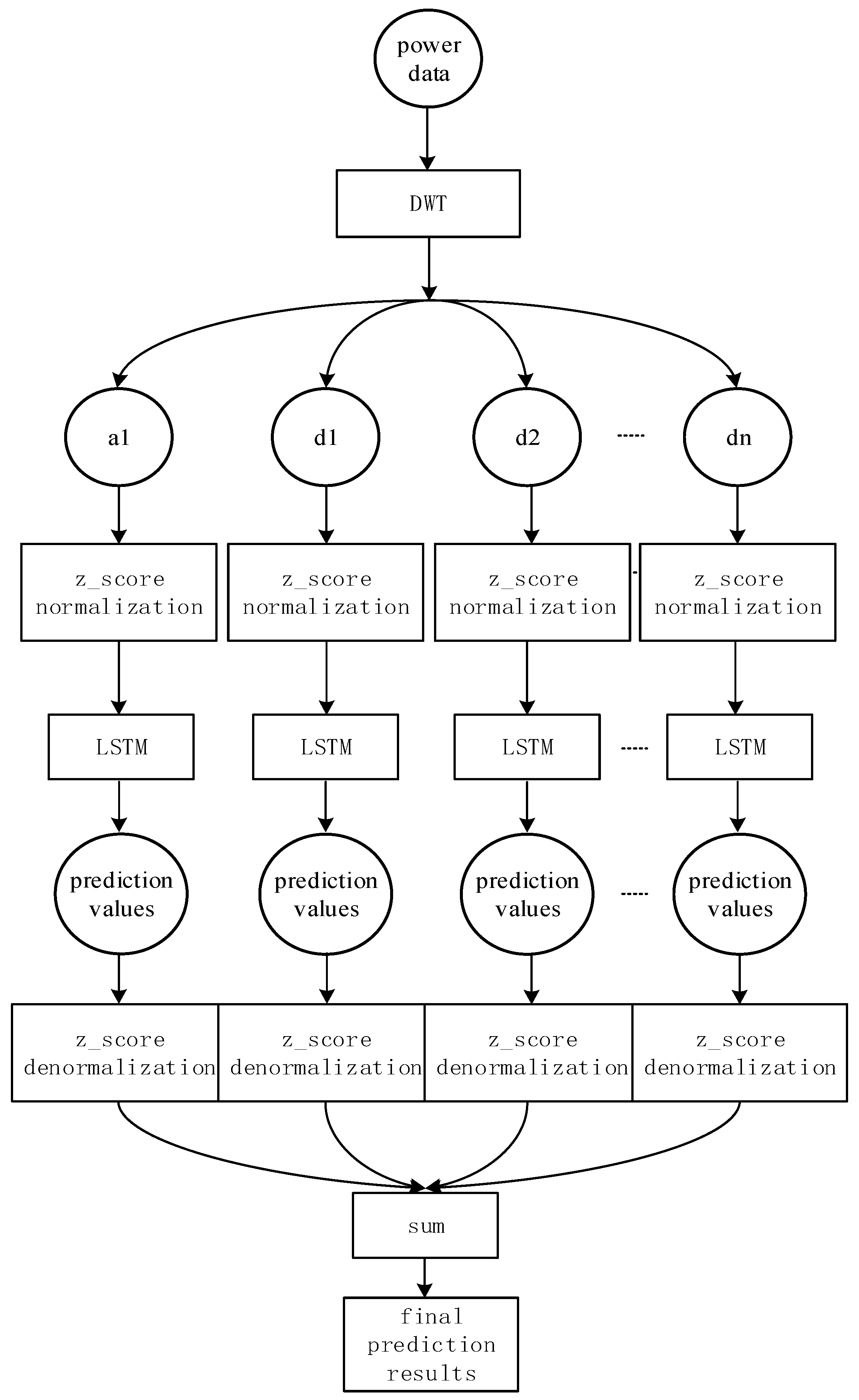
3.1. Sketch of DWT_LSTM

The proposed DWT_LSTM forecasting method has two important components: the LSTM and DWT. The two components are used to implement the strategy of dividing and conquering. Specifically, the proposed method uses DWT to decompose original wind power data into sub-signals and independent LSTMs to learn the temporal relationship from sub-signals, respectively.

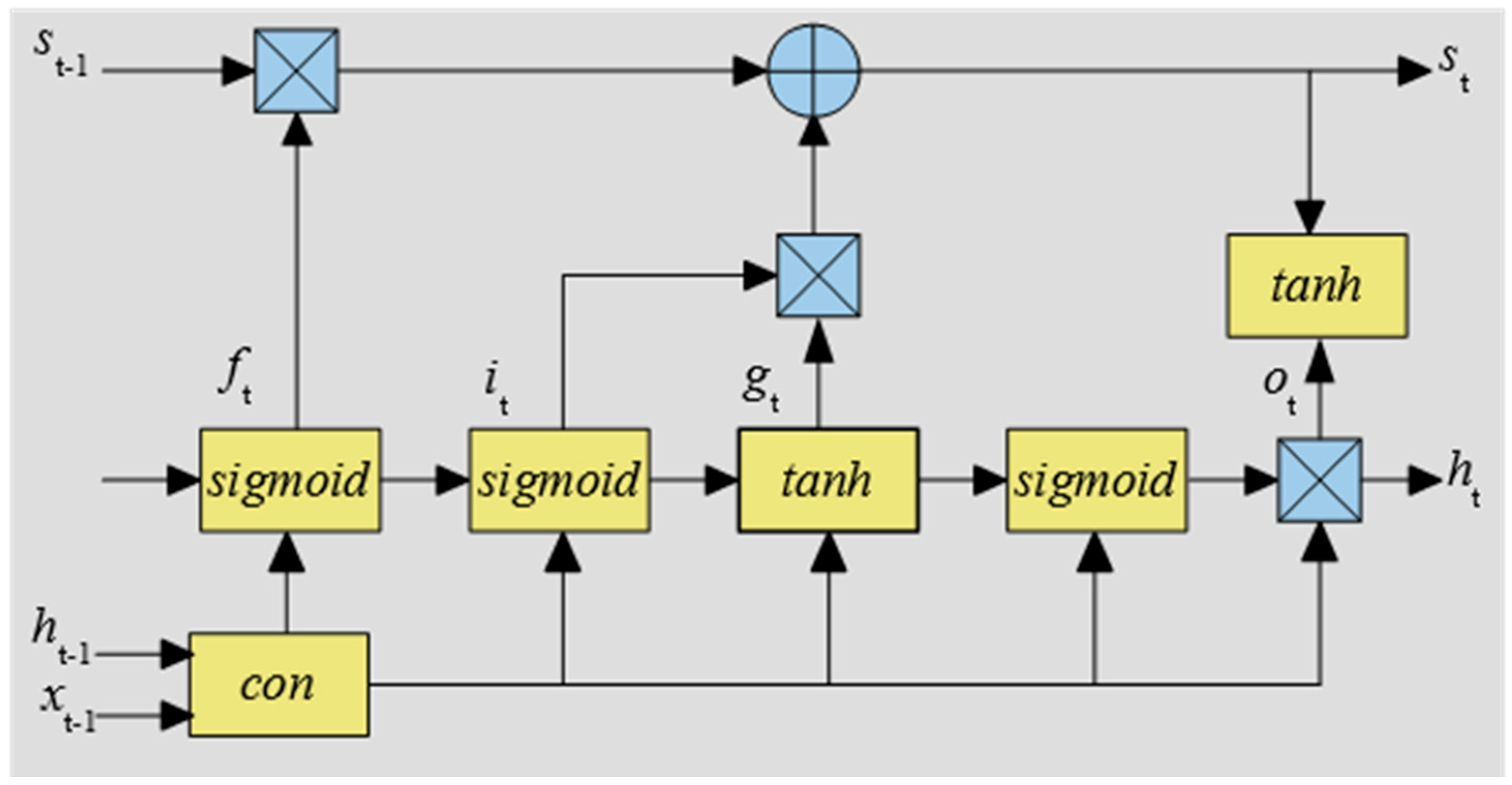
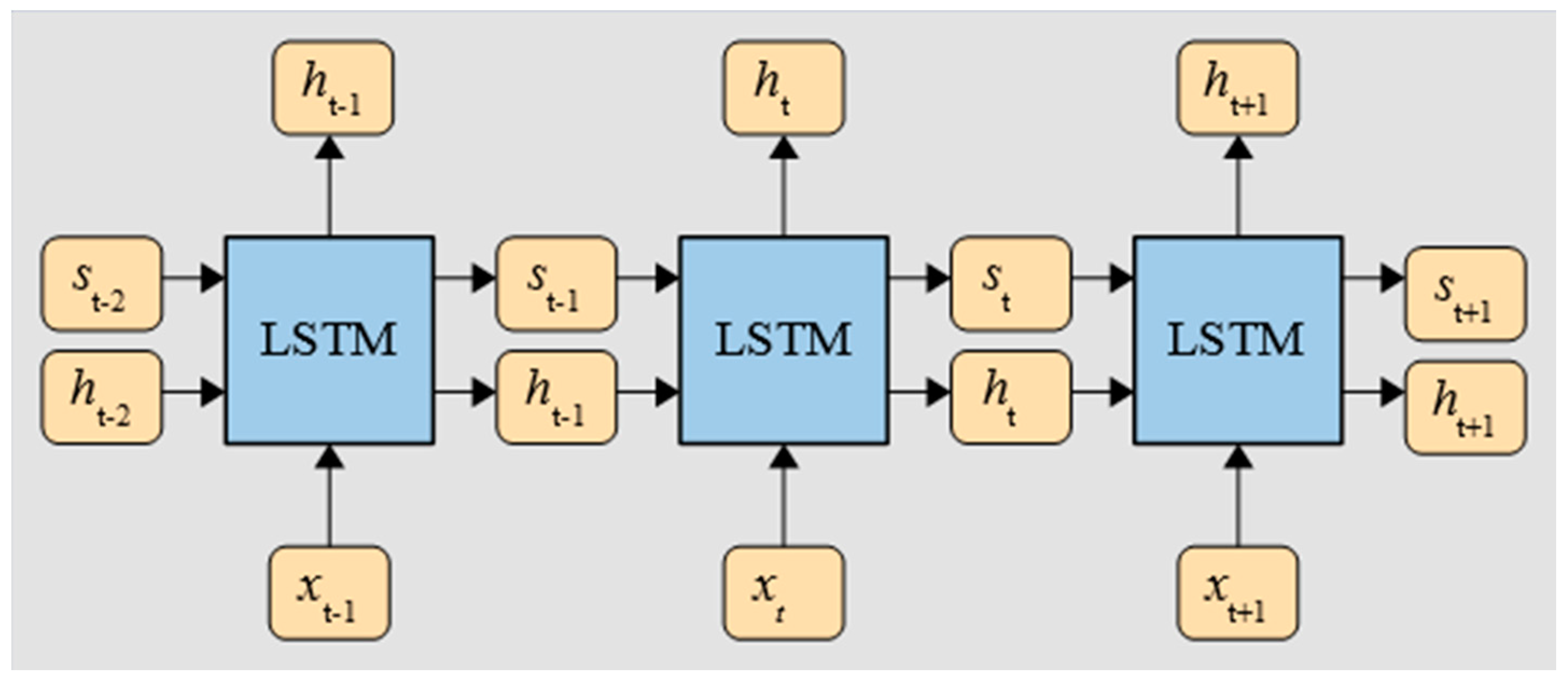
3.2. Long Short-Term Memory (LSTM)

The long short-term memory network (LSTM), which is a variant of RNN, was proposed in 1997 [36]. An LSTM unit shown in Figure 1 is composed of a cell, an input gate, an output gate, and a forget gate. The unique structure of LSTM can effectively solve the problems of gradient disappearance and gradient explosion problems in the training process of RNN.

The plus sign in Figure 1 denotes the addition of element levels, the multiplication sign denotes element level multiplication, and con presents vector merge. ${\mathit{f}}_{\mathit{t}}$, ${\mathit{i}}_{\mathit{t}}$, ${\mathit{g}}_{\mathit{t}}$, ${\mathit{o}}_{\mathit{t}}$ present the forgotten gate, the input gate, the input node, and the output gate, respectively. The dependencies relationship between the data in the input sequence is caught by the cell. The input gate controls the extent of the values which flow into the cell. The forget gate controls the extent of the values which remain in the cell. The values in the cell are used to calculate the output activation of the LSTM; its extent is controlled by the output gate.

The calculation formulas related to the LSTM structure in Figure 1 are:

$${\mathit{f}}_{\mathit{t}}= \sigma \left({\mathit{W}}_{\mathit{f}}\left[{\mathit{h}}_{\mathit{t}-\mathbf{1}},{\mathit{x}}_{\mathit{t}}\right]+{\mathit{b}}_{\mathit{f}}\right)$$

(6)

$${\mathit{i}}_{\mathit{t}}= \sigma \left({\mathit{W}}_{\mathit{i}}\left[{\mathit{h}}_{\mathit{t}-1},{\mathit{x}}_{\mathit{t}}\right]+{\mathit{b}}_{\mathit{i}}\right)$$

(7)

$${\mathit{g}}_{\mathit{t}}= tanh\left({\mathit{W}}_{\mathit{g}}\left[{\mathit{h}}_{\mathit{t}-\mathbf{1}},{\mathit{x}}_{\mathit{t}}\right]+{\mathit{b}}_{\mathit{g}}\right)$$

(8)

$${\mathit{o}}_{\mathit{t}}= \sigma \left({\mathit{W}}_{\mathit{o}}\left[{\mathit{h}}_{\mathit{t}-\mathbf{1}},{\mathit{x}}_{\mathit{t}}\right]+{\mathit{b}}_{\mathit{o}}\right)$$

(9)

$${\mathit{s}}_{\mathit{t}} = {\mathit{s}}_{\mathit{t}-\mathbf{1}}\odot {\mathit{f}}_{\mathit{t}}+{\mathit{g}}_{\mathit{t}}\odot {\mathit{i}}_{\mathit{t}}$$

(10)

$${\mathit{h}}_{\mathit{t}}=\tanh \left({\mathbf{s}}_{\mathit{t}}\right)\odot {\mathit{o}}_{\mathit{t}}$$

(11)

In Equations (6)–(11), ${\mathit{W}}_{\mathit{f}}$, ${\mathit{W}}_{\mathit{i}}, {\mathit{W}}_{\mathit{g}},{\mathit{W}}_{\mathit{o}}$ are the corresponding weight matrix connecting the input signal $\left[{\mathit{h}}_{\mathit{t}-\mathbf{1}},{\mathit{x}}_{\mathit{t}}\right]$, and $\odot$ represents the element level multiplication. σ represents the sigmoid activation function, and tanh represents the hyperbolic tangent function. The state (${\mathit{s}}_{\mathit{t}}$) of cell remembers previous values over arbitrary time intervals and the three gates control the flow of information into and out of the cell. Thus, the LSTM network is very suitable for prediction problems based on a time sequence. Hence, this paper uses LSTM to fit the approximation function $\widehat{f}$ mentioned in Formula (3). The schematic diagram of the LSTM network training is shown in Figure 2.

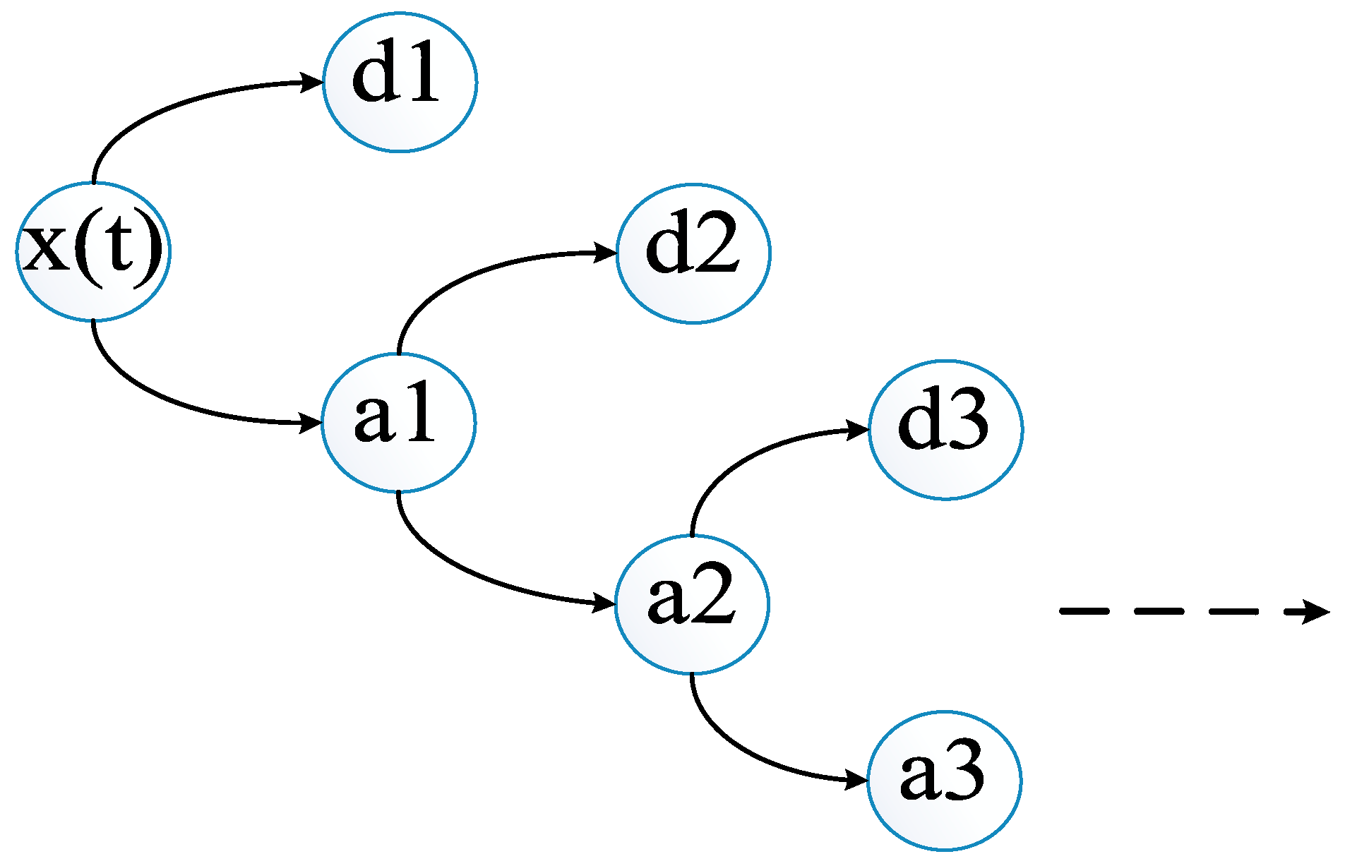
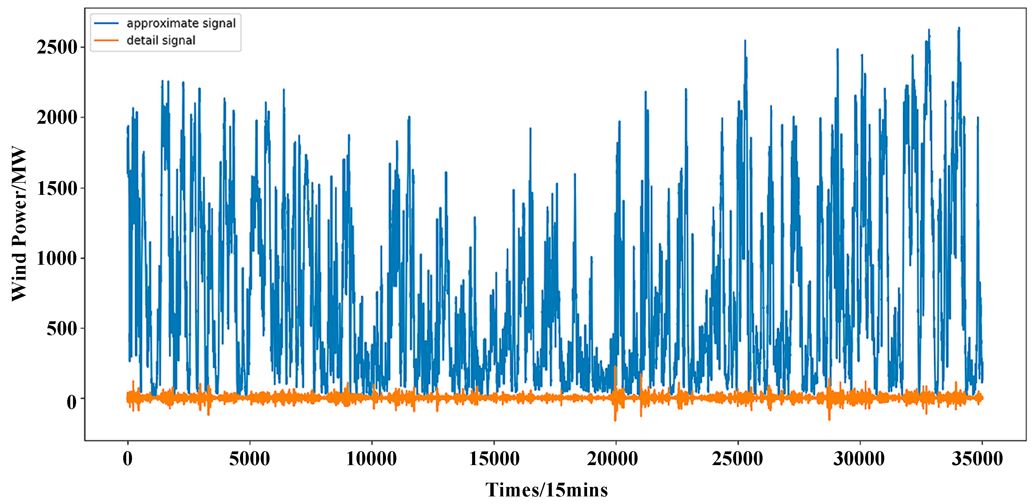
3.3. Discrete Wavelet Transform (DWT)

Considering that the wind power generation is caused by a variety of natural factors, including wind speed, wind direction, air density, air pressure, and wind turbine friction, the output power series of the wind turbine is non-stationary, volatile, and time-ordered. The influence of these factors on output power are different. The wind speed and wind direction are the two major factors affecting the wind power generation. The wind power signal contains the components of various frequencies: the contribution of the low-frequency components and high-frequency components of wind power data are of different importance to its dynamic behavior.

If these components with different frequencies can be learned by independent LSTMs respectively, the performance of data mining will be improved. Thus, the divide and conquer strategy requires the decomposition of the original wind power data into low-frequency sub-signal and high-frequency sub-signal by a proper decomposition algorithm.

This paper uses the discrete wavelet transform for decomposing the original wind power data. It uses a time-scale function to analyze data, so that wavelet transform has multi-scale resolution and time-shifting characteristics. Scaling operations can observe signals on different scales. Therefore, the wavelet transform is very suitable for dealing with non-stationary time series problems including wind power data.

Assuming that the square of x(t) can be integral, x(t) can be expanded under a wavelet basis function. This operation is called a continuous wavelet transform of x(t). The mathematical definition of the wavelet basis function is:

$${\Psi }_{a,b}\left(t\right) = \frac{1}{\sqrt{|a|}}\Phi (\frac{t-b}{a}),a\ne 0,b\in R.$$

(12)

The mathematical definition of continuous wavelet transform of x(t) is:

$$W_x\left(a,b\right)=< x\left(t\right),{\Psi }_{a,b}\left(t\right) >=\frac{1}{\sqrt{|a|}}{\displaystyle {\int }_R}{x}_t\left(t\right)\overline{\Phi (\frac{t-b}{a})}dt.$$

(13)

In Equations (12) and (13), a represents the scale parameter, and b represents the time center parameter. When a and b change continuously, the whole transformation process is called continuous wavelet transform. However, in practical applications, the continuous transformation which greatly increases the computational complexity, application cost, and the implementation difficulty, is actually replaced by discrete wavelet transform (DWT) with a small step size.

Discrete wavelet transform makes the application of wavelet transform easy to be put into practice. It discretizes the a and b parameters exponentially, which reduces the computational complexity and avoids the information redundancy caused by continuous wavelet transform. The discrete wavelet transform of x(t) is defined as:

$$W_x\left(j,k\right) = < x\left(t\right),{\Psi }_{j,k}\left(t\right) > = \frac{1}{\sqrt{|a|}}{\displaystyle {\int }_R}{x}_t\left(t\right)\overline{\Phi (\frac{t-b}{a})}dt.$$

(14)

In Formula (14), a and b are discrete, $a=a_0^j$, $b=k{a}_0^j{b}_0$, $a_0>1$, $b_0>0$, $j\in Z$, $k\in Z$.

The algorithm for discrete wavelet transform is the Mallat algorithm proposed in 1988. It is actually a signal decomposition method. For the multi-resolution characteristics of wavelets, the variable j is used to determine the resolution at different scales. Specifically, the main contour of the original signal is observed on a large scale, and the detailed information of the original signal are observed on a small scale. Finally, the decomposition results are obtained by the stepwise increase of j: one approximate signal (i.e., low-frequency components) and n (the value of n needs to be set by a human) detail signals (i.e., high frequency) $d_n,d_{n-1},d_{n-2}\dots ,d_1$. The original signal and the two types of sub-signals are satisfied by the following equation:

$$x\left(t\right) = a_n+d_n+d_{n-1}+\dots +d_1.$$

(15)

A schematic diagram of discrete wavelet transform decomposition is shown in Figure 3.

3.4. The Proposed DWT_LSTM Method

This section presents the DWT_LSTM prediction method, as shown in Figure 4. The method mainly has two stages: the preprocessing of original wind power data, and the training and forecasting of sub-signal data.

Wind power data are divided into a training set, a validation set, and a test set according to the order of the time series. The training set, validation set, and test set account for 70%, 20%, and 10% of the original data, respectively. Approximate signal and detail signal values vary widely, which is not conducive to the training of LSTM. Therefore, the z score normalization method shown in Equation (16) was used to standardize the decomposed data in this paper. The normalized data z(t) obeys the standard normal distribution.

$$z\left(t\right)=\frac{x^{\prime }\left(t\right)-x_{mean}^{\prime }}{x_{std}^{\prime }}$$

(16)

$x^{\prime }\left(t\right)$ represents one of the sub-signals ($a_n,d_1\cdots d_n$), $x_{mean}^{\prime }$ and $x_{std}^{\prime }$ are the mean and standard deviation of $x^{\prime }\left(t\right)$, respectively.

After the training of the LSTMs, each sub-signal of the test set was predicted, and the normalized predicted value $p\left(t\right)$ of each sub-signal was obtained. Then $p\left(t\right)$ was denormalized to $y\left(t\right)$ of the corresponding sub-signal. The formula of $y\left(t\right)$ is shown in Equation (17).

$$y\left(t\right)=p\left(t\right)\ast x_{std}^{\prime }+x_{mean}^{\prime }$$

(17)

Finally, the wind power prediction results of the original data were obtained by superimposing all denormalized predicted values $y\left(t\right)$.

4. Experimental Design

4.1. Benchmarks and Hyperparameter Settings

In order to verify the performances of the DWT_LSTM method proposed in this paper, five algorithms including DWT_RNN, DWT_BP, LSTM, RNN, and BP were selected as benchmarks. The proposed forecasting method DWT_LSTM and the five benchmarks were classified into two groups: group 1 includes DWT_LSTM, DWT_RNN, and DWT_BP; group 2 includes LSTM, RNN, and BP. Obviously, all the forecasting algorithms of group 1 contain the discrete wavelet transform operation, while the members of group 2 contain only the corresponding neural networks of group 1. Group 1 shows the influence of discrete wavelet transform on prediction accuracy, and group 2 was used to find the most suitable neural network of LSTM, RNN, and BP for the time series prediction problem.

The hyperparameters were set as follows: the number of input layer nodes and the number of the hidden layer nodes in the neural network of the six methods mentioned above were all set to 10, based on repeated experiments. The wind power generation prediction belongs to the regression problem, so the output layer of the neural network of the six methods does not have to set the activation function. The iteration period (epoch) was uniformly set to 100.

To make the experiment more persuasive, for each of the six methods, experiments with the prediction step size from one to five were carried out.

4.2. Optimization Algorithm

Deep learning often requires a lot of time and computational resources for training, which is a major driving force for the development of the optimization algorithm.

Although distributed parallel training can be adopted to accelerate the deep learning, the required computational resources will not be drastically reduced. Hence, only the optimization algorithm that consumes less computational resources and makes the model converge faster can fundamentally accelerate the learning speed and improve the forecasting performances of the neural network. The Adam optimizer was introduced for this reason [47] as a further development of the stochastic gradient descent algorithm. The Adam algorithm can update the weights of the neural network iteratively based on the training data. Since only first-order gradients were needed, the stochastic gradient descent maintains a fixed learning rate (i.e., alpha) to update all weights. Adam designs an independent adaptive learning rate for different parameters by calculating the first-order moment estimation and the second-order moment estimation of the gradient. The Adam algorithm includes the advantages of two random gradient descent extensions: AdaGrad and RMSProp. The adaptive gradient algorithm (AdaGrad [48]) retains a learning rate for each parameter to improve the performance of the sparse gradient; and the RMSProp [49] maintains the learning rate adaptively for each parameter based on the mean value of the nearest weight gradient. Adam not only calculates the learning rate of adaptive parameters based on the first-order moment mean, but also makes full use of the gradient second-order moment mean. Adam is a first-order optimization algorithm that can replace the traditional stochastic gradient descent algorithm.

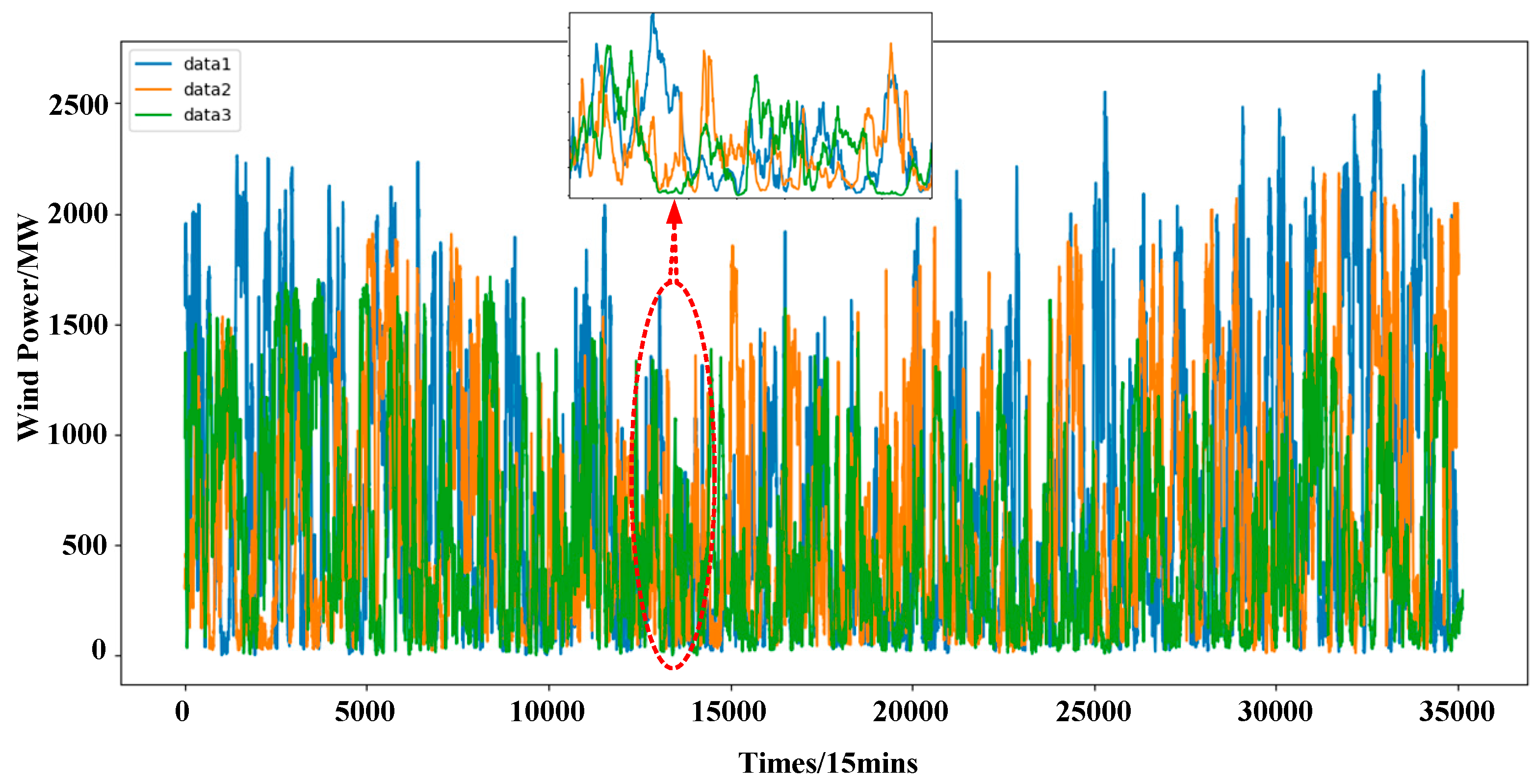
4.3. Data Description

Three time series wind power data from three different wind farms were selected for experiments in this paper. Every time series covered 12 months in order to make experiments more supportive. The time interval between two neighboring power data was 15 min (35,000 points in total). The parameter of the wind power data was MW. Three wind farms were located in inner Mongolia (farm 1), The Netherlands (farm 2), and Yunnan of China (farm 3), respectively. These wind farms were far away enough to ensure that the three time series wind power data were different. The three different data are shown in Figure 5.

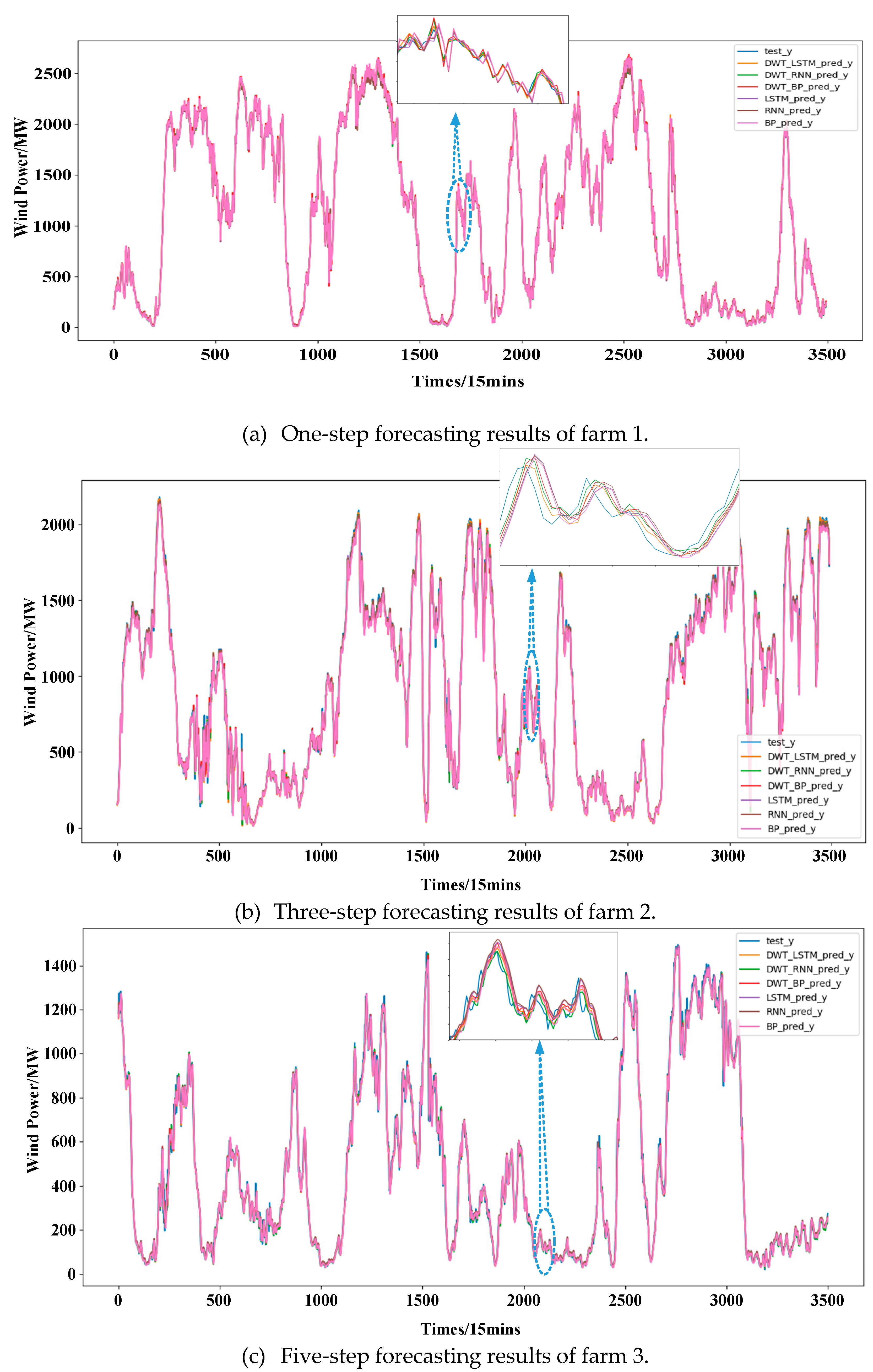
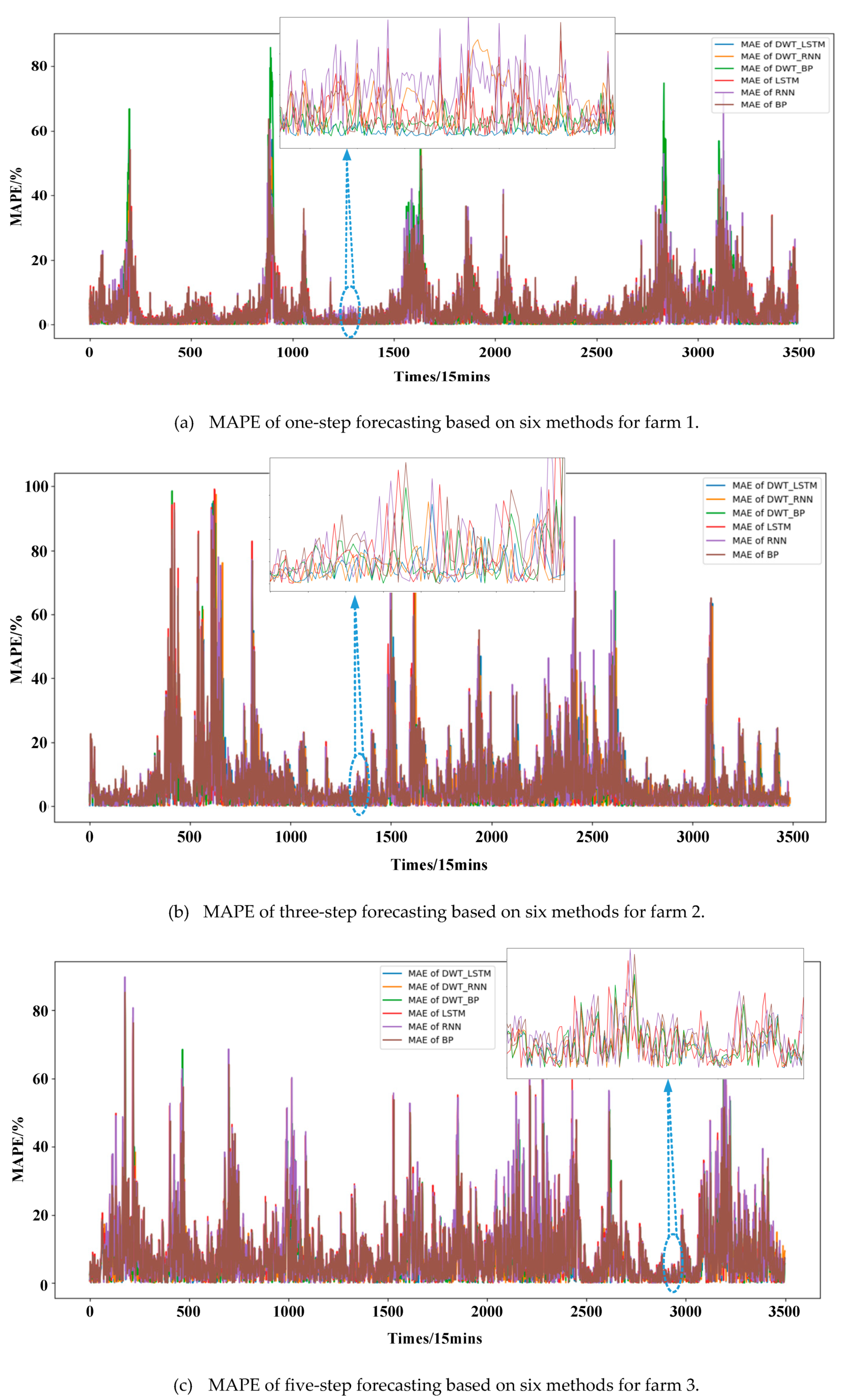
5. Results and Analysis

The experimental results confirm that the db7 wavelet function was suitable for decomposing and reconstructing the wind power raw data shown in Figure 5 to obtain an approximate signal and one detail signal, as shown in Figure 6.

Figure 7 shows one-step forecasting results of wind farm 1, three-step forecasting results of wind farm 2, and five-step forecasting results of wind farm 3. It can be seen that the prediction accuracy of the proposed method is the best compared with the benchmarks.

Figure 8 shows the mean absolute percentage error (MAPE) of one-step forecasting for farm 1, the MAPE of three-step forecasting for farm 2, and the MAPE of five-step forecasting for farm 3. The MAPE of the proposed method was the lowest.

In order to further verify the validity and performance of the proposed prediction method, three evaluation indexes including the mean absolute error (MAE), the mean absolute percent error (MAPE), and the root mean square error (RMSE), were selected to evaluate the performance of every method according to Equations (18)–(20). The experimental results including MAE, MAPE, and RMSE of the original data test set are shown in

Table 1. Evaluation indexes of farm 1. RNN: recurrent neural network; BP: back-propagation; MAE: mean absolute error; RMSE: root mean square error.

Prediction Step	Algorithms	MAE/MW	MAPE/%	RMSE/MW
1	DWT_LSTM	10.12	3.01	14.22
	DWT_RNN	13.95	3.41	21.23
	DWT_BP	16.42	4.85	22.80
	LSTM	28.31	4.80	39.27
	RNN	29.10	5.17	40.51
	BP	32.26	5.53	41.66
2	DWT_LSTM	18.98	4.01	27.11
	DWT_RNN	26.27	4.29	40.08
	DWT_BP	28.53	4.55	44.96
	LSTM	24.83	3.39	35.43
	RNN	29.93	7.45	50.48
	BP	34.57	5.79	52.83
3	DWT_LSTM	29.48	5.15	41.33
	DWT_RNN	30.66	6.33	43.51
	DWT_BP	36.51	6.98	51.08
	LSTM	40.73	7.41	59.02
	RNN	41.23	7.81	61.26
	BP	46.59	8.92	65.15
4	DWT_LSTM	37.70	6.66	53.32
	DWT_RNN	40.23	7.02	58.11
	DWT_BP	43.19	8.77	62.96
	LSTM	47.18	8.13	68.51
	RNN	46.65	8.52	68.54
	BP	50.75	8.61	71.04
5	DWT_LSTM	45.23	8.10	63.22
	DWT_RNN	46.36	11.54	63.67
	DWT_BP	55.87	12.34	75.11
	LSTM	54.32	9.91	77.12
	RNN	55.01	10.27	78.96
	BP	56.42	10.79	77.52

,

Table 2. Evaluation indexes of farm 2.

Prediction Step	Algorithms	MAE/MW	MAPE/%	RMSE/MW
1	DWT_LSTM	11.26	2.02	17.35
	DWT_RNN	12.16	2.60	17.57
	DWT_BP	14.27	2.79	22.51
	LSTM	28.78	5.07	46.08
	RNN	29.97	5.17	46.20
	BP	30.18	5.19	46.11
2	DWT_LSTM	21.11	3.52	32.13
	DWT_RNN	24.84	3.95	34.26
	DWT_BP	25.23	4.68	38.28
	LSTM	36.71	6.56	55.32
	RNN	37.23	6.79	56.02
	BP	37.86	6.91	56.52
3	DWT_LSTM	28.55	5.31	43.6
	DWT_RNN	29.64	5.40	44.09
	DWT_BP	35.97	6.74	52.18
	LSTM	43.70	8.05	64.87
	RNN	44.75	8.16	66.05
	BP	47.27	8.32	68.35
4	DWT_LSTM	38.13	6.96	55.91
	DWT_RNN	39.24	7.17	56.34
	DWT_BP	46.68	8,12	67.65
	LSTM	48.91	9.02	72.88
	RNN	51.83	9.33	74.65
	BP	52.00	9.78	75.16
5	DWT_LSTM	44.52	8.36	64.62
	DWT_RNN	44.73	8.77	65.21
	DWT_BP	48.10	9.08	70.99
	LSTM	55.71	10.17	81.56
	RNN	58.29	10.21	83.33
	BP	59.78	10.59	84.09

and

Table 3. Evaluation indexes of farm 3.

Prediction Step	Algorithms	MAE/MW	MAPE/%	RMSE/MW
1	DWT_LSTM	5.49	1.75	8.64
	DWT_RNN	5.63	1.89	8.67
	DWT_BP	8.96	3.64	12.95
	LSTM	15.23	4.41	24.13
	RNN	15.28	4.41	24.16
	BP	15.74	4.94	24.33
2	DWT_LSTM	10.21	3.04	15.75
	DWT_RNN	10.40	3.11	15.96
	DWT_BP	13.12	3.95	20.29
	LSTM	18.36	5.43	28.62
	RNN	18.96	5.48	29.41
	BP	19.77	6.87	29.44
3	DWT_LSTM	15.27	4.35	22.92
	DWT_RNN	15.82	5.36	23.46
	DWT_BP	19.71	7.66	28.15
	LSTM	22.80	6.65	34.95
	RNN	23.35	6.67	35.17
	BP	23.92	8.42	35.32
4	DWT_LSTM	19.85	5.77	29.73
	DWT_RNN	20.08	6.75	29.89
	DWT_BP	22.94	6.76	34.37
	LSTM	25.96	7.65	39.83
	RNN	26.47	8.62	39.84
	BP	26.71	8.71	39.96
5	DWT_LSTM	23.96	7.11	35.83
	DWT_RNN	24.20	7.20	36.22
	DWT_BP	26.67	8.48	40.01
	LSTM	29.27	8.61	44.10
	RNN	30.14	10.01	44.13
	BP	30.26	10.06	44.96

.

$$MAE=\frac{1}{N}{\displaystyle \sum _{i=1}^N}|y\_rea{l}_i-y\_pre{d}_i|$$

(18)

$$MAPE=\frac{1}{N}{\displaystyle \sum _{i=1}^N}\left|\frac{y\_rea{l}_i-y\_pre{d}_i}{y\_rea{l}_i}\right|\ast 100$$

(19)

$$RMSE=\sqrt{\frac{{\displaystyle {\sum }_{i=1}^N}{\left(y\_rea{l}_i-y\_pre{d}_i\right)}^2}{N}}$$

(20)

In the Equations (18)–(20), $y\_rea{l}_i$ and $y\_pre{d}_i$ represent the real power generation and predicted power generation at time i, respectively.

Take Table 1 for example—the analysis of evaluation index is as follows:

(1) For any prediction step size, MAE, MAPE, and RMSE of DWT_LSTM were lower than DWT_RNN, DWT_BP, LSTM, RNN, and BP, so the prediction performance of DWT_LSTM proposed in this paper is the best. Taking the experimental results of one step as an example, the MAE of DWT_LSTM was sequentially reduced by 27.46%, 38.37%, 64.25%, 65.22%, and 68.63%, respectively, compared with DWT_RNN, DWT_BP, LSTM, RNN, and BP; the MAPE of DWT_RNN, DWT_BP, LSTM, RNN, and BP was sequentially reduced by 11.73%, 37.94%, 37.29%, 41.78%, and 45.57%; the RMSE of DWT_RNN, DWT_BP, LSTM, RNN, and BP was sequentially reduced by 33.01%, 37.63%, 63.80%, 64.90%, and 65.87%. It can be seen that compared with the other five prediction methods, the prediction accuracy of DWT_LSTM was significantly improved, which indicates that the application of discrete wavelet transform enables independent LSTMs to more fully dig the major information and minor information contained in the approximate signal and the detail signal, respectively. Obviously, the discrete wavelet transform improves the prediction accuracy of wind power indeed.

(2) For any prediction step size, among the three algorithms of LSTM, RNN, and BP, LSTM had the lowest MAE, MAPE, and RMSE, and its prediction performance was optimal. Taking the experimental results of one step as an example, the MAE of LSTM was decreased by 2.71% and 12.24%, respectively, compared with RNN and BP; the MAPE of LSTM was decreased by 7.16% and 13.20%, respectively, compared to RNN and BP; the RMSE of LSTM was decreased by 3.06% and 5.74%, respectively, compared to RNN and BP. The experimental results demonstrate that LSTM is more suitable for time series wind power prediction problems than RNN and BP neural networks because the unique structure of LSTM can learn the temporal relationship contained in input sequences better.

Analysis of Table 2 and Table 3 shows the same conclusions as Table 1. However, for the brevity of this paper, they were not demonstrated.

6. Conclusions

This paper proposed a DWT_LSTM prediction method based on the divide and conquer strategy. The DWT was used to decompose original wind power data into sub-signals, the main information. The independent LSTM was designed to approximate the temporal dynamic behaviors of the sub-signals respectively.

With the proposed prediction method, the main information that was contained in the approximated wind power sub-signal and the minor information contained in detailed wind power sub-signals can be identified by different LSTMs more efficiently. Also, the temporal relationship contained in the input sequence data can be learned through independent LSTMs. The experimental results show that the proposed prediction method has the best prediction accuracy compared with the benchmarks.

In future work, the optimizer algorithm of LSTM can be further improved to enhance the learning ability for time series prediction. In addition, DWT_LSTM is an accurate forecasting method that can be used as a reference for the prediction of other renewable energy power generation.

References

1. Cerna, F.V.; Pourakbari-Kasmaei, M.; Contreras, J.; Gallego, L.A. Optimal Selection of Navigation Modes of HEVs considering CO2 Emissions Reduction. IEEE Trans. Veh. Technol. 2019. [Google Scholar] [CrossRef]
2. Sun, Y.; Hou, X.; Yang, J.; Han, H.; Su, M.; Guerrero, J.M. New perspectives on droop control in AC microgrid. IEEE Trans. Ind. Electron. 2017, 64, 5741–5745. [Google Scholar] [CrossRef]
3. Li, L.; Sun, Y.; Liu, Z.; Hou, X.; Shi, G.; Su, M. A Decentralized Control with Unique Equilibrium Point for Cascaded-type Microgrid. IEEE Trans. Sustain. Energy 2019, 10, 310–326. [Google Scholar] [CrossRef]
4. Reinders, A.; Übermasser, S.; van Sark, W.; Gercek, C.; Schram, W.; Obinna, U.; Lehfuss, F.; van Mierlo, B.; Robledo, C.; van Wijk, A. An Exploration of the Three-Layer Model Including Stakeholders, Markets and Technologies for Assessments of Residential Smart Grids. Appl. Sci. 2018, 8, 2363. [Google Scholar] [CrossRef]
5. Alsadi, S.; Khatib, T. Photovoltaic Power Systems Optimization Research Status: A Review of Criteria, Constrains, Models, Techniques, and Software Tools. Appl. Sci. 2018, 8, 1761. [Google Scholar] [CrossRef]
6. Uribe-Pérez, N.; Hernández, L.; de la Vega, D.; Angulo, I. State of the art and trends review of smart metering in electricity grids. Appl. Sci. 2016, 6, 68. [Google Scholar] [CrossRef]
7. Crossland, A.; Jones, D.; Wade, N.; Walker, S. Comparison of the Location and Rating of Energy Storage for Renewables Integration in Residential Low Voltage Networks with Overvoltage Constraints. Energies 2018, 11, 2041. [Google Scholar] [CrossRef]
8. Irmak, E.; Ayaz, M.S.; Gok, S.G.; Sahin, A.B. A survey on public awareness towards renewable energy in Turkey. In Proceedings of the International Conference on Renewable Energy Research and Application (ICRERA), Milwaukee, WI, USA, 19–22 October 2014; pp. 932–937. [Google Scholar]
9. Olowu, T.; Sundararajan, A.; Moghaddami, M.; Sarwat, A. Future Challenges and Mitigation Methods for High Photovoltaic Penetration: A Survey. Energies 2018, 11, 1782. [Google Scholar] [CrossRef]
10. Home-Ortiz, J.M.; Melgar-Dominguez, O.D.; Pourakbari-Kasmaei, M.; Mantovani, J.R. A stochastic mixed-integer convex programming model for long-term distribution system expansion planning considering greenhouse gas emission mitigation. Int. J. Electr. Power Energy Syst. 2019, 108, 86–95. [Google Scholar] [CrossRef]
11. Liang, H.; Liu, Z.; Liu, H. Stabilization Method Considering Disturbance Mitigation for DC Microgrids with Constant Power Loads. Energies 2019, 12, 873. [Google Scholar] [CrossRef]
12. Safari, N.; Chen, Y.; Khorramdel, B.; Mao, L.P.; Chung, C.Y. A spatiotemporal wind power prediction based on wavelet decomposition, feature selection, and localized prediction. In Proceedings of the IEEE Electrical Power and Energy Conference (EPEC), Saskatoon, SK, Canada, 22–25 October 2017; pp. 1–6. [Google Scholar]
13. Hou, X.; Sun, Y.; Han, H.; Liu, Z.; Yuan, W.; Su, M. A fully decentralized control of grid-connected cascaded inverters. IEEE Trans. Sustain. Energy 2019, 10, 310–317. [Google Scholar] [CrossRef]
14. Hou, X.; Sun, Y.; Zhang, X.; Zhang, G.; Lu, J.; Blaabjerg, F. A Self-Synchronized Decentralized Control for Series-Connected H-bridge Rectifiers. IEEE Trans. Power Electron. 2019. [Google Scholar] [CrossRef]
15. Song, D.R.; Fan, X.; Yang, J.; Liu, A.; Chen, S.; Joo, Y. Power extraction efficiency optimization of horizontal-axis wind turbines through optimizing control parameters of yaw control systems using an intelligent method. Appl. Energy 2018, 224, 267–279. [Google Scholar] [CrossRef]
16. Song, D.R.; Li, Q.; Cai, Z.; Li, L.; Yang, J.; Su, M.; Joo, Y.H. Model predictive control using multi-step prediction model for electrical yaw system of horizontal-axis wind turbines. IEEE Trans. Sustain. Energy 2018. [Google Scholar] [CrossRef]
17. Su, M.; Liu, Z.; Sun, Y.; Han, H.; Hou, X. Stability Analysis and Stabilization methods of DC Microgrid with Multiple Parallel-Connected DC-DC Converters loaded by CPLs. IEEE Trans. Smart Grid 2018, 9, 142–149. [Google Scholar] [CrossRef]
18. Liu, Z.; Su, M.; Sun, Y.; Han, H.; Hou, X.; Guerrero, J.M. Stability analysis of DC microgrids with constant power load under distributed control methods. Automatica 2018, 90, 72–90. [Google Scholar] [CrossRef]
19. Liu, Z.; Su, M.; Sun, Y.; Yuan, W.; Han, H. Existence and Stability of Equilibrium of DC Microgrid with Constant Power Loads. IEEE Trans. Power Syst. 2018, 33, 7011–7033. [Google Scholar] [CrossRef]
20. Li, L.; Ye, H.; Sun, Y.; Han, H.; Li, X.; Su, M.; Guerrero, J.M. A communication-free economical-sharing scheme for cascaded-type microgrids. Int. J. Electr. Power Energy Syst. 2019, 104, 1–9. [Google Scholar] [CrossRef]
21. Liu, Z.; Su, M.; Sun, Y.; Li, L.; Han, H.; Zhang, X.; Zheng, M. Optimal criterion and global/sub-optimal control schemes of decentralized economical dispatch for AC microgrid. Int. J. Electr. Power Energy Syst. 2019, 104, 38–42. [Google Scholar] [CrossRef]
22. Haque, A.U.; Nehrir, M.H.; Mandal, P. A hybrid intelligent model for deterministic and quantile regression approach for probabilistic wind power forecasting. IEEE Trans. Power Syst. 2014, 29, 1663–1672. [Google Scholar] [CrossRef]
23. Yu, Z. Research on Wind Power Prediction and Optimization Algorithm Based on Neural Network. Master’s, Thesis, Jiangsu University, Zhenjiang, China, 2016. [Google Scholar]
24. Shi, Z.; Liang, H.; Dinavahi, V. Direct interval forecast of uncertain wind power based on recurrent neural networks. IEEE Trans. Sustain. Energy 2018, 9, 1177–1187. [Google Scholar] [CrossRef]
25. Bouzidi, L. Wind power variability: Deterministic and probabilistic forecast of wind power production. In Proceedings of the Saudi Arabia Smart Grid (SASG), Jeddah, Saudi Arabia, 12–14 December 2017; pp. 1–7. [Google Scholar]
26. Shuang-Lei, F.; Wei-Sheng, W.; Chun, L.I.; Hui-zhu, D.A. Study on the physical approach to wind power prediction. Proc. CSEE 2010, 30, 1–6. [Google Scholar]
27. Xiao, Y.S.; Wang, W.Q.; Huo, X.P. Study on the Time-series Wind Speed Forecasting of the Wind farm Based on Neural Networks. Energy Conserv. Technol. 2007, 25, 106–108. [Google Scholar]
28. Yang, X.; Xiao, Y.; Chen, S. Wind speed and generated power forecasting in wind farm. Proc.-Chin. Soc. Electr. Eng. 2005, 25, 1. [Google Scholar]
29. Ding, Z.; Yang, P.; Yang, X.; Zhang, Z. Wind power prediction method based on sequential time clustering support vector machine. Autom. Electr. Power Syst. 2012, 36, 131–135. [Google Scholar]
30. Lipton, Z.C.; Berkowitz, J.; Elkan, C. A critical review of recurrent neural networks for sequence learning. arXiv, 2015; arXiv:1506.00019. [Google Scholar]
31. Wang, L.J.; Dong, L.; LIAO, X.Z.; Gao, Y. Short-term power prediction of a wind farm based on wavelet analysis. Proc. CSEE 2009, 28, 006. [Google Scholar]
32. Ming, D.; Li, Z.; Yi, W.U. Wind speed forecast model for wind farms based on time series analysis. Electr. Power Autom. Equip. 2005, 25, 32–34. [Google Scholar]
33. Olaofe, Z.O.; Folly, K.A. Wind power estimation using recurrent neural network technique. In Proceedings of the IEEE Power and Energy Society Conference and Exposition in Africa: Intelligent Grid Integration of Renewable Energy Resources (Power Africa), Johannesburg, South Africa, 9–13 July 2012; pp. 1–7. [Google Scholar]
34. Kolen, J.F.; Kremer, S.C. Gradient Flow in Recurrent Nets: The Difficulty of Learning Long Term. Dependencies 2001, 28, 237–243. [Google Scholar]
35. Bengio, Y.; Simard, P.; Frasconi, P. Learning long-term dependencies with gradient descent is difficult. IEEE Trans. Neural Netw. 2002, 5, 157–166. [Google Scholar] [CrossRef] [PubMed]
36. Hochreiter, S.; Schmidhuber, J. Long short-term memory. Neural Comput. 1997, 9, 1735–1780. [Google Scholar] [CrossRef] [PubMed]
37. Jin, L.W.; Zhong, Z.Y.; Yang, Z.; YANG, W.X.; XIE, Z.C.; SUN, J. Applications of deep learning for handwritten Chinese character recognition: A review. Acta Autom. Sin. 2016, 42, 1125–1141. [Google Scholar]
38. Kotecha, N.; Young, P. Generating Music using an LSTM Network. arXiv, 2018; arXiv:1804.07300. [Google Scholar]
39. Chen, X.; Wu, Z.; Yu, J. TSSD: Temporal Single-Shot Object Detection Based on Attention-Aware LSTM. arXiv, 2018; arXiv:1803.00197v2. [Google Scholar]
40. Qian, Q.; Huang, M.; Lei, J.; Zhu, X. Linguistically Regularized LSTM for Sentiment Classification. In Proceedings of the Meeting of the Association for Computational Linguistics, Vancouver, BC, Canada, 30 July–4 August 2017; pp. 1679–1689. [Google Scholar]
41. Graves, A.; Jaitly, N.; Mohamed, A.R. Hybrid speech recognition with deep bidirectional LSTM. In Proceedings of the IEEE Workshop on Automatic Speech Recognition and Understanding, Olomouc, Czech Republic, 8–12 December 2013; pp. 273–278. [Google Scholar]
42. Zhu, Q.; Hongyi, L.I.; Wang, Z.; Chen, J.F.; Wang, B. Short-Term Wind Power Forecasting Based on LSTM. Power Syst. Technol. 2017, 12, 3797–3802. [Google Scholar]
43. Prasetyowati, A.; Sudiana, D.; Sudibyo, H. Comparison Accuracy W-NN and WD-SVM Method in Predicted Wind Power Model on Wind Farm Pandansimo. In Proceedings of the 4th International Conference on Nano Electronics Research and Education (ICNERE), Hamamatsu, Japan, 27–29 November 2018; pp. 27–29. [Google Scholar]
44. Safari, N.; Chung, C.Y.; Price, G.C. Novel multi-step short-term wind power prediction framework based on chaotic time series analysis and singular spectrum analysis. IEEE Trans. Power Syst. 2018, 33, 590–601. [Google Scholar] [CrossRef]
45. RAN, Q.W. Applications of Wavelet Transform and Fractional Fourier Transform Theory; Harbin Institute of Technology Press: Harbin, China, 2001. [Google Scholar]
46. Li, S.X. Wavelet Transform and Its Application; Higher Education Press: Beijing, China, 1997. [Google Scholar]
47. Kingma, D.P.; Ba, J. Adam: A method for stochastic optimization. arXiv, 2014; arXiv:1412.6980. [Google Scholar]
48. Mukkamala, M.C.; Hein, M. Variants of rmsprop and adagrad with logarithmic regret bounds. In Proceedings of the 34th International Conference on Machine Learning, Sydney, NSW, Australia, 6–11 August 2017; Volume 70, pp. 2545–2553. [Google Scholar]
49. Ida, Y.; Fujiwara, Y.; Iwamura, S. Adaptive learning rate via covariance matrix based preconditioning for deep neural networks. arXiv, 2016; arXiv:1605.09593. [Google Scholar]
Figure 1. The structure of the long short-term memory (LSTM) unit.
Applsci 09 01108 g001
Figure 2. The training process of LSTM.
Applsci 09 01108 g002
Figure 3. The Mallet decomposition algorithm.
Applsci 09 01108 g003
Figure 4. The forecasting process of the discrete wavelet transform and long short-term memory network (DWT_LSTM).
Applsci 09 01108 g004
Figure 5. Power values generated by the wind turbine registered every 15 mins.
Applsci 09 01108 g005
Figure 6. Results of DWT for wind farm 1.
Applsci 09 01108 g006
Figure 7. Forecasting results of the six methods.
Applsci 09 01108 g007
Figure 8. Mean absolute percentage error (MAPE) of wind power forecasting.
Applsci 09 01108 g008