SLA-Based Adaptation Schemes in Distributed Stream Processing Engines ^†

Abstract

With the upswing in the volume of data, information online, and magnanimous cloud applications, big data analytics becomes mainstream in the research communities in the industry as well as in the scholarly world. This prompted the emergence and development of real-time distributed stream processing frameworks, such as Flink, Storm, Spark, and Samza. These frameworks endorse complex queries on streaming data to be distributed across multiple worker nodes in a cluster. Few of these stream processing frameworks provides fundamental support for controlling the latency and throughput of the system as well as the correctness of the results. However, none has the ability to handle them on the fly at runtime. We present a well-informed and efficient adaptive watermarking and dynamic buffering timeout mechanism for the distributed streaming frameworks. It is designed to increase the overall throughput of the system by making the watermarks adaptive towards the stream of incoming workload, and scale the buffering timeout dynamically for each task tracker on the fly while maintaining the Service Level Agreement (SLA)-based end-to-end latency of the system. This work focuses on tuning the parameters of the system (such as window correctness, buffering timeout, and so on) based on the prediction of incoming workloads and assesses whether a given workload will breach an SLA using output metrics including latency, throughput, and correctness of both intermediate and final results. We used Apache Flink as our testbed distributed processing engine for this work. However, the proposed mechanism can be applied to other streaming frameworks as well. Our results on the testbed model indicate that the proposed system outperforms the status quo of stream processing. With the inclusion of learning models like naïve Bayes, multilayer perceptron (MLP), and sequential minimal optimization (SMO)., the system shows more progress in terms of keeping the SLA intact as well as quality of service (QoS).

1. Introduction

Contemporary data-intensive applications necessitate the persistent increment in the power of computing resources and the volume of storage devices which are in many real-life use cases essential on-demand for a specific operation in data lifecycle such as data collection, extraction, processing, and reporting. Additionally, it needs to be elastically scaled up and down according to the incoming workload. Cloud computing [1] delivers platforms and environments for data-intensive applications and facilitates the effective use of big data technologies and distributed resources [2]. Given the large volume of data to be transmitted and processed, each phase of the data-intensive applications is bringing new challenges to the underlying networking architecture and services.

Distributed batch processing systems like MapReduce [3] and Hadoop [4] still serve an essential function in the processing of static and historical datasets. However, MapReduce and Hadoop are not suitable for streaming data applications, because they were designed with the philosophy of offline batch processing of static data in focus, in which all the input data need to be stored in a distributed file system in advance. Streaming data processing systems gained significant attention due to the reason that processing a large volume of data in the batch is often not sufficient in use cases where new data has to be processed fast to quickly adapt and react to changes, such as intrusion detection, fraud detection, and Web analytics systems. Ideally, streaming engines must be capable of handling vast; ever-changing data streams in real-time and of conveying results to potential clients with a minimum delay. Several steaming engines including Storm [5], Spark [6], Samza [7], Google Data Flow [8], and Flink [9] have been developed for this very purpose; to support the dynamic analytics of the streaming datasets. These distributed processing systems handle both the batch and real-time analytics which represent the core of modern big data applications. These frameworks orchestrate numerous nodes structured in a cluster and distribute the workload through communication using different messing techniques.

Flink is an open-source, distributed, dynamic streaming engine, designed to process valid and limitless data streams in a user-friendly environment [9]. Flink is unique in that it does a lot for stream processing what Hadoop has done for batch processing [10]. Flink was founded on the belief that the various functions of data processing applications, such as dynamic stream analytics, continuous data pipelines, batch processing of historic data, and iterative algorithms, such as machine learning and graph analysis, can all be performed through utilizing fault-tolerant data streams. Regardless of the fact that recent streaming engines have solved a majority of the issues plaguing big data analytics [11], there are still a few difficult hurdles to overcome, namely, window correctness and buffer timeout. In retrospect, some of the recent streaming engines provide a level of support for the latency and throughput of the system, and the reliability of the results produced, but none have come close to providing a quick runtime.

The default Flink framework, as well as other streaming engines, have presented some inventive challenges for both the academic and industrial communities. Firstly, there’s always either a stagnant configuration procedure or no established procedure to set the maximum out-of-order capacity for any incoming window, as well as a fixed technique for the task tracker’s buffering timeout, all of which are crucial towards the execution of any streaming processing system. Secondly, the majority of these frameworks are incapable of maintaining the latency of these tasks at runtime, causing all manner of problems for the performance of many sensitive and critical applications, such as fraud detection in a banking system, online traffic checking, and so on. Thirdly, default topologies are always mapped to the nodes, whether the knowledge of the workloads is known or not, creating an overhead and resulting in a dip in performance, not only at the task at hand but also in the system as a whole. To rectify these challenges, we propose and extend the idea of our previous work [12] that has the aptitude of utilizing a variety of different metrics such as late element frequency in the incoming workload, as well as both currently recorded throughput of the system and the runtime measured latency value to control the inherent latency problem as quickly and as efficiently as possible. Unlike the default system, it makes the task tracker’s buffering timeout and max out-of-order-ness dynamic, which can be changed and maintained according to the Service Level Agreements (SLAs) with the users. We propose three varying modes: automated, semi-automated, and manual, to successfully maintain the trade-off between latency and throughput using max-out-of-order-ness and window correctness. In case of manual mode, the system require the administrator to provide target latency, priority proportion of throughput and correctness, lower limit of throughput, and lower limit of window correctness to decide and forward the decision to the streaming environment. Semi-automate mode requires the administrator to provide target latency and preferred throughput, while in automated mode the system only needs target latency as an input.

Following suit from our proposal, Section 2 highlights the aforementioned problem we must handle, and Section 3 introduces our proposed system. Section 4 explains a detailed use-case scenario, Section 5 offers a thorough evaluation of our work, Section 6 describes some similar projects, and Section 7 concludes the paper.

2. Use Case Scenario: Fraud Detection

With the increase of online merchants and e-commerce, fraud becomes a trillion dollar problem for the global economy with the loss of 3.5 to 4 trillion dollars per year, which makes about 5% of global GDP [13]. Several fraud detections and prevention companies are working to detect and prevent such fraud on time including BankCard USA, Kount, Ingenico, and fraud.net.

The system of fraud.net is one of the world’s leading peer production-based fraud prevention framework which aggregate and analyze large amounts of fraud data from thousands of online merchant in real time. This collaborative program is the largest merchant-led effort to combat online payment fraud costing US merchants an estimated amount of 20 billion dollars annually. It protects more than 2% of all the US-based e-commerce, and its clientele is growing very fast each year recently. This framework saves up to one million dollars a week for its customers by helping them detect and prevent fraud.

The primary challenge of such platforms is to build and train a more significant number of more targeted and precise machine learning models to counter the effect of increasingly different and evolving forms of fraud. As the fraudster’s strategy changes with time, the system should be able to evolve itself with the fraud evolution. There might be 100 different fraud schemes and each one with 100 different variations at any given day. To tackle these issues, the platform needs to have machine learning models and capabilities to identify and handle a new fraud scheme, as it pops up including its different variations.

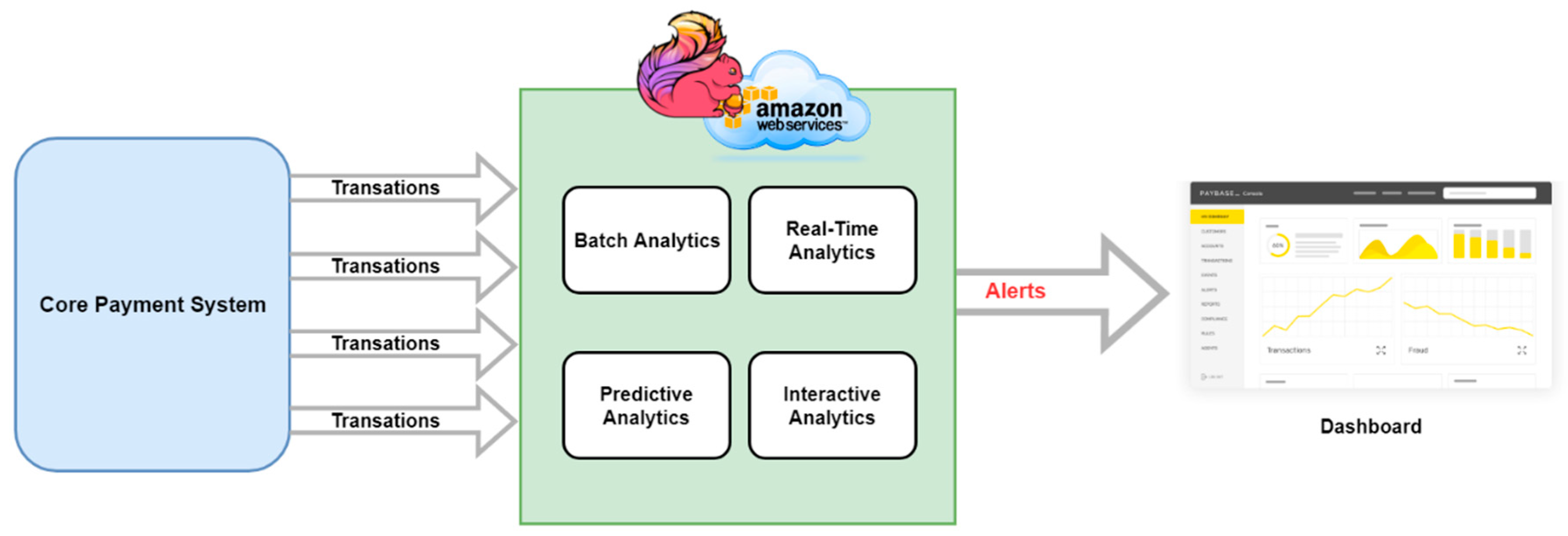
Latency-sensitive applications like fraud detection, traffic analysis, and media streaming need to adapt these capabilities and achieve a better tradeoff between lower latency and higher throughput. With this the goal of the system, the proposed system has different variations of the algorithm to achieve a better tradeoff between these, while taking SLA agreement into consideration. A generic fraud detection and prevention system architecture is shown in Figure 1. The core payment system process all the transaction and pass it to the main detection and prevention system. The system contains batch analytics, real-time analytics, predictive analytics, and interactive analytics modules which process the transactional data and produce alerts based on the analysis of the incoming workload. The alerts are then portrayed to the dashboard, and the system admin takes actions accordingly.

3. Problem Definition

3.1. Problem Statement

Big data applications have exploded in popularity and usage over the years, and to complement this rise, distributed streaming engines like Flink, Samza, and Storm among others, have emerged to process this massive amount of data in a quick, scalable, and reliable way, through distributing both finite and infinite data streams in real-time across the worker nodes of a cluster. Flink, in particular, enables the replication of the operators of a job graph, each with their own code and properties, such as parallelism, across a cluster, decreasing latency and improving both throughput and performance.

Flink code is given, in dataflow form, to the graph builder, which transforms it into a dataflow graph and passes it on to the client, who communicates with the Job Manager using its actor system, as seen in Figure 2. The Job Manager is responsible for scheduling and resource management, essentially keeping track of distributed tasks, scheduling proceeding tasks, and responding to completed or failed tasks, all whilst coordinating every deployment, including for standalone and YARN clusters. The dataflow graph is representation of the jobs as combinations of distributed tasks connected to each other to form a job, and so on, i.e., a job is the combination of tasks to be distributed among available task tracker within the cluster. During job execution, the Job Manager keeps track of distributed tasks, decides when to schedule the next task or set of tasks, and reacts to finished or failed tasks. Job Manager receives a representation of data flow and intermediate results operators (such as joins after the use of Flat map operator, etc.) in the form of job graph. Each operator has its properties like parallelism, and the code it executes. The Job Manager transforms the received job graph into an execution graph according to the parallelism and available resources in the cluster.

All Task Managers have at least one task slot, which primarily runs a pipeline of parallel tasks, or a group of numerous consecutive tasks (i.e., tasks such as map, reduce, and union), and Flink can execute these tasks simultaneously [14]. On a cluster with two task managers, each containing three slots, operators could be distributed amongst the slots, as shown in Figure 3, and are assigned according to the SLA-based parallelism offered by the system. Seeing as latency and throughput are inversely proportional to one another, streaming engines require a feature that can provide an equal trade-off between both.

3.2. Definition of Terms

3.2.1. Max-Out-Of-Orderness

Max-Out-Of-Orderness defines the maximum amount of time that an element(s) for a particular window of timestamp “t” is allowed to be late, by at most “n” milliseconds, after the earliest arriving element of that window, before being ignored in the computation of a final result for said window. As an example, the maxOutOfOrderness is set to value 6000, meaning that elements are allowed to be late for a maximum of six seconds while not being ignored in the final results as shown in Figure 4.

3.2.2. Buffer Timeout

The buffer timeout is the maximum wait time allocated to the buffers to receive data before its transfer between machines occurs, even if the buffer was not full, and while benefiting throughput, it can cause latency issues. An example of this is if the buffer timeout is set to a value of 500 ms in an attempt to increase the throughput of the system, while that of the default value of it is 100 ms as shown in Figure 5. This longer timeout results in a potentially slower performance, so to counteract this, there are two extreme cases where we can maximize throughput at the cost of latency without severely affecting the system: either by setting the Buffer Timeout value to anywhere close to zero (a value of zero can cause a severe performance degradation), or by setting it to “−1”, effectively removing the timeout and simply waiting for the buffers to fill.

3.2.3. Subtask

Programs in Apache Flink (and the others) are inherently distributed and parallel in nature. Incoming data streams are split into partitions, and operators into operator subtasks that execute independently from each other, the number of which is determined based on the parallelism of the operator. An example of this is a streaming dataflow with a condensed and parallelized view of the source, map and apply methods with parallelism two and sink with parallelism one as shown in Figure 6. Streams can transport data between two operators in either a forwarding or a redistributing pattern; forwarding streams preserve the partitioning and order of the elements, while a redistributing stream changes the partitioning of the streams (as seen below in Figure 6 between map() and keyBy/window/apply operators).

3.2.4. Correctness

One often thinks of correctness in terms of accuracy, which is right in translation, but not entirely so in the context of the computing world, where correctness is the accuracy of the answers; if an answer is accurate, but slow to achieve, it is difficult to assume that it is correct.

Flink supports four notions of time for data processing, namely, event time, storage time, ingestion time and processing time, as shown in Figure 7, which highlights where each of the four is recorded and used. Event time is as the name suggests, the time where all events on the device occurred, recorded before the stream enters the system, while storage time is the arrival time of the events into the message queue. Ingestion time is recorded when events enter the system, and each record gets the source’s current time as ingestion timestamp at the source operator, while processing time refers to the current system time of the main machine executing the operations. For example, if an application run at hourly processing time window, and application begins at 8:25 am, the first hourly processing time window will only include the events processed between 8:25 am and 9:00 am, and the next window will include the events processed between 9:00 am and 10:00 am, and so on.

While modern streaming engines are capable of using event time windows to reflect the occurrence of events, system elements can be delayed at a moment’s notice, making it difficult to pinpoint the entire series of events that occur in a specific timestamp; these elements are known as late elements. As a result, these modern distributed systems have two critical drawbacks, namely, the increased amount of data buffering and the aforementioned point about late elements. Flink handles these issues through its use of watermarks, which marks the progress of events throughout the flow of data using timestamps, giving us a more reliable, hands-on estimate of a window’s completeness. Watermarks tend to use the available information such as partition ordering within partitions, among others, to produce an accurate progress estimate, but as seen in Figure 8, this can easily backfire, resulting in the appearance of late elements and an inaccurate estimation. As in this case, the stream is an out of order stream, and two late elements occur due to their arrival after the specified watermark accordingly. Late elements can be defined through a watermark as the elements with the timestamp less than or equal to the current watermark at the time of their arrival. Window correctness is vital towards meeting a user-defined SLA like end-to-end latency or throughput for the above reasons.

4. Proposed System

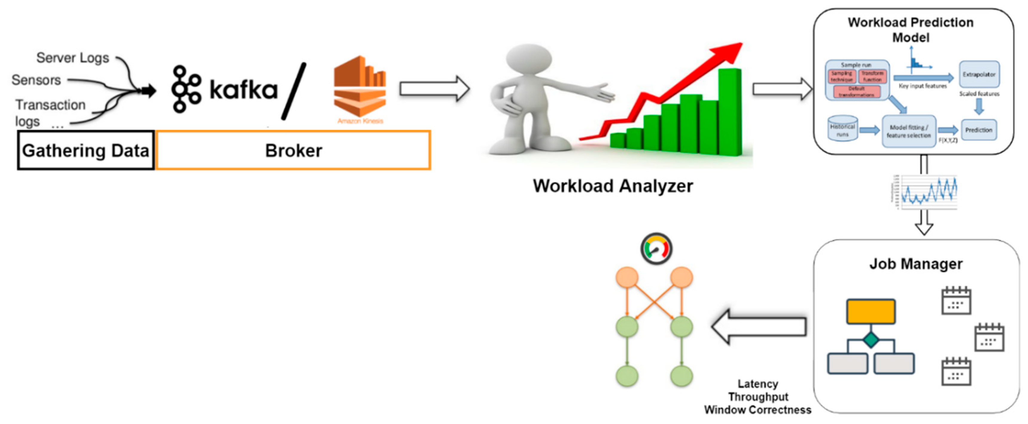
The proposed streaming data processing system is an extended version of our preliminary research work [12], containing brokering module, workload analyzer, and job manager latency controller. Whereas the extended work in this article is composed of input gathering module, brokering module, workload analyzer, a workload prediction module, and job manager’s latency-throughput controller module as shown in Figure 9. The input gathering module is the data and event entry point to the system. It collects data from a variety of sources, like sensors, sensor logs, transaction logs, and the like, which are then passed on to a data broker, such as Kafka or Amazon Kinesis. The data broker backup the data streams in varieties of ways, offer the streams for consumption by the engine, as well as provide the stream recovery mechanism. It also has the role to pipeline this newly acquired data stream to the workload analyzer module. This module uses the incoming workload to analyze and measure the metric values used in the analytic algorithms of the system. It also has the ability to analyze and correlate streams, create derived streams and states. The workload analyzer then passes the resultant metrics and calculated information to the workload prediction module and other upstream modules. The workload prediction module is designed based around machine learning algorithms and previous research on the subject for any multi-tier architecture system [15,16]. This module gives the system a sense of the incoming workload to make the Job Manager ready and help keeps the system from breaching the SLA agreement. The job manager then takes this collective information, along with the incoming prediction from the previous module and the decision algorithm, to calculate an improved performance enhancement. The system can then increase or decrease both throughput and latency accordingly (using any of the target latency modes described in Section IV-D). Once the system reaches the necessary SLA requirement (if possible), the algorithm will steadily reduce maxOutOfOrderness and bufferTimeOut, until a status queue between latency and throughput is established. Furthermore, we have designed an adaptive topology refinement scheme to get the benefit of topological changes needed to be made by the system at runtime while taking the incoming workload into account, which is not in the scope of this paper and will be discussed in our upcoming article.

To this end, we propose a complex adaptive system (CAS), an adaptive watermark and buffer time-out mechanism designed for the efficient optimization of the Flink engine. In the upcoming section, we will briefly highlight the metrics used for our proposed optimization of Flink, as well as explain our aimed latency-bound algorithm. Furthermore, we will also elaborate on the concept surrounding the dynamic buffering timeout and the various target latency techniques we have used throughout the project.

4.1. Performance Metrics

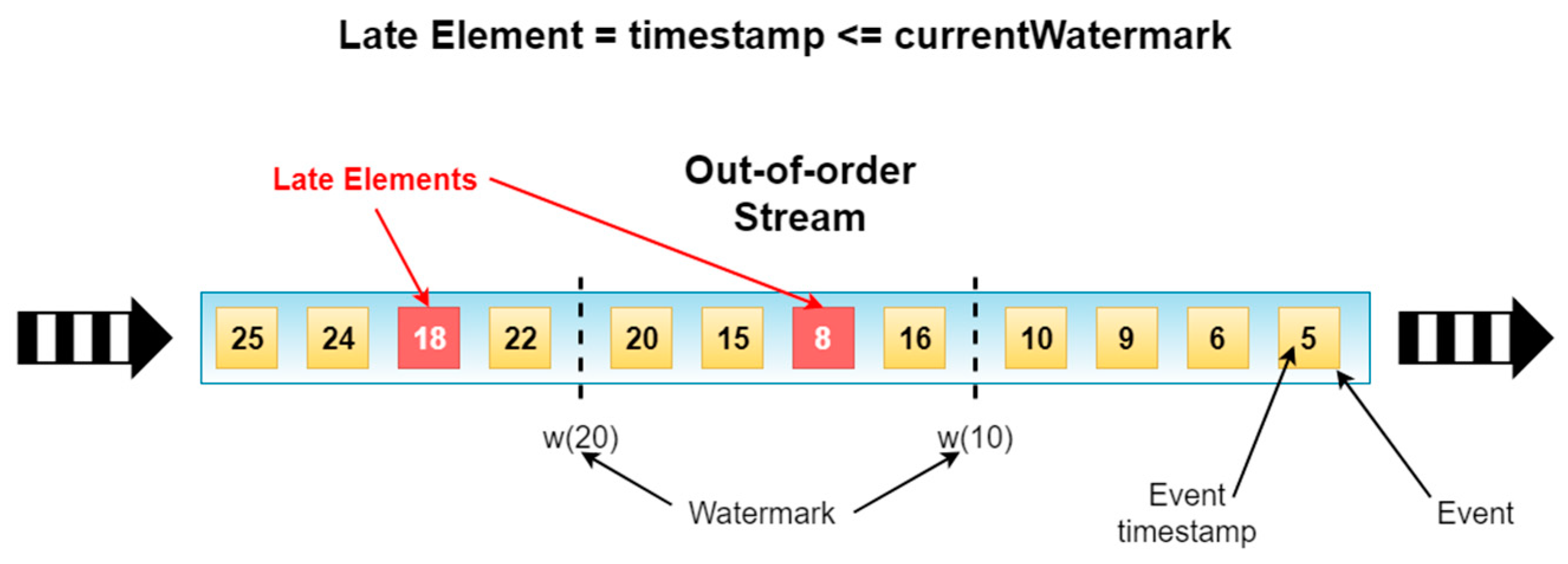
4.1.1. Late Elements Frequency

Within the window operators, whenever a subtask receives any late elements, the operator will alert the master, which in this case is the Job Manager, of the arrival of such elements. The master will then compile the number of late elements of the system, including the recent arrivals, and use them, later on, to help determine the tradeoff mentioned at the beginning of the section between latency and throughput.

4.1.2. Throughput

Flink bestows all users with a rich metric API set. Using Operator.numRecordsOut(the number of accumulated records) at the sink operator to compute the average throughput per second by dividing the result of the numRecordsOut function of Operator class by the time passed in seconds as in Equation (1):

Throughput = Ň/T

(1)

where Ň is the result of the Operator.numRecordsOut, while T is the time in seconds.

4.1.3. Latency

It is genuinely challenging to gather the latency in the entire stream as it is a complex metric. Therefore, it is achieved through sample slicing off some of the records from the incoming stream, followed by an appropriate estimation. Records sampling is completed as well, to prevent any potential degradation of performance in the system, and specific records are marked from the source location, enabling the sink operator to identify them during calculation, as these records are the only ones required.

Marking can be done randomly (through random selection algorithm), or at specified times depending on circumstance. This way, the sink operator know the exact records to use in latency calculations. The Job Manager (master node) calculate the latency through following Equation (2).

$$Latency= t_{finish}- t_{start}$$

(2)

where $t_{finish}$ is the finish time of the marked sample and $t_{start}$ is the entering time of the sample record in the execution pipeline.

4.2. Latency Control Mechanism

Latency control mechanism acts as an addition towards the Job Manager’s ability to find the suboptimal balance between latency, throughput and window correctness, through considering a variety of metrics in the process of achieving the objective of minimalizing latency while maximizing throughput as much as possible. Latency is decreased when the number of out-of-order events that reach the system also decreases, while throughput increases based on the value of the buffering timeout. The main concern here was to sub-optimally decide the tradeoff between latency, window correctness and buffering timeout, to ensure that the system would be able to maintain its functioning without the breach of SLA agreement. We focus on the tradeoff as an increase of throughput can cause latency to be a breach of SLA, or it can also hurt window correctness (as correctness is sometimes more about timely getting the result than only getting the accurate results).

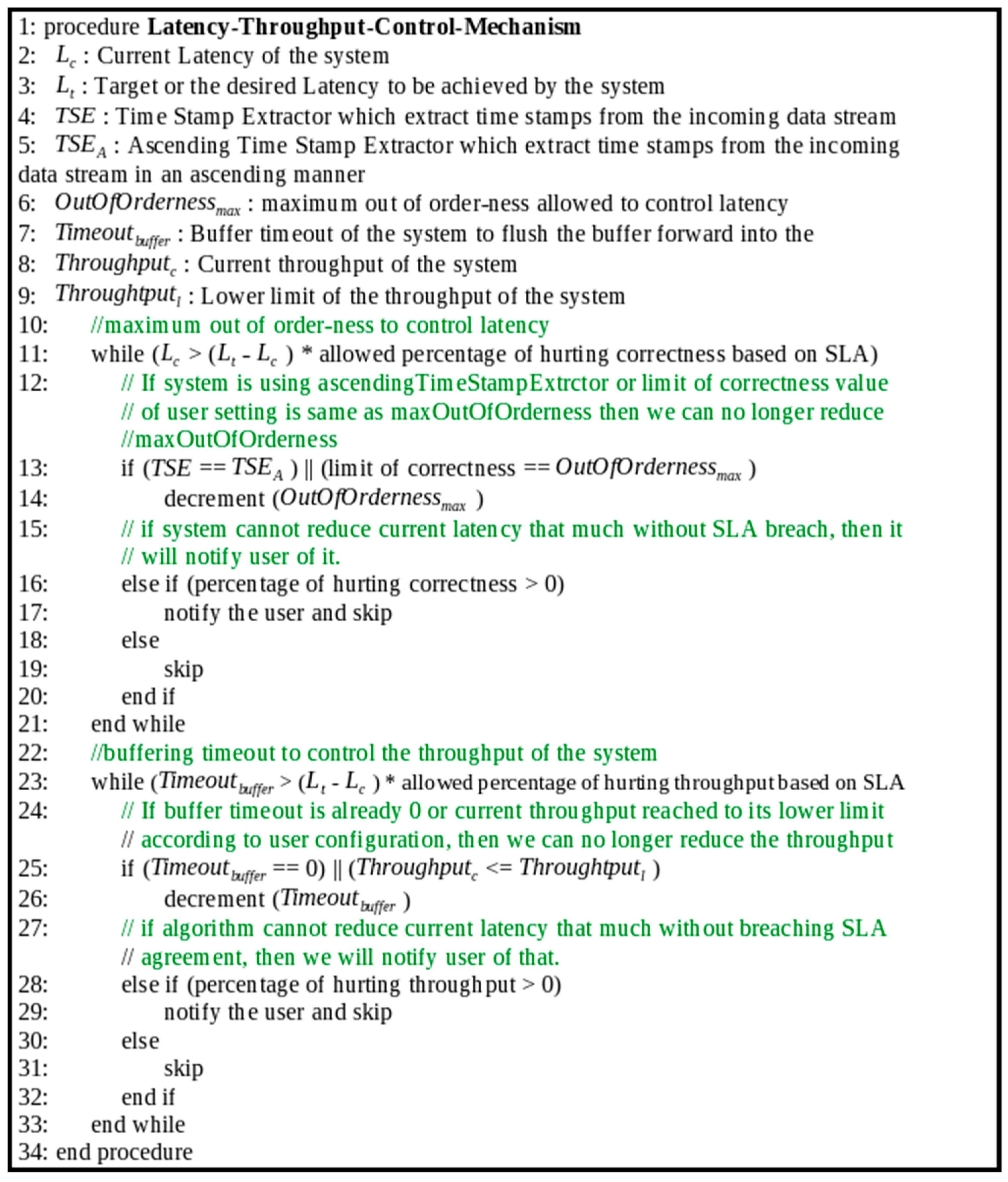
Through using our proposed metric system, as seen in section III-B, the Job Manager now has an educated estimation of the appearance rate of late elements and a vision of the system as a whole in real-time. The master then triggers the algorithm in Figure 10 upon the overflow of the user’s targetLatencyBound.

The algorithm in Figure 10 is self-explanatory, and it controls the latency and throughput of the cluster on run time. The algorithm first uses the allowed range of maximumOfOrderness to control latency of the system and confirms whether the maxOutOfOrderness can be reduced or not, which could result in one of two possible outcomes. The first possible outcome, if the system is using ascendingTimeStampExtractor or the limitation of the correctness value declared by the user is the same as maxOutOfOrderness, then the reduction is no longer possible, and this step is then bypassed. The second outcome happens if the system can reduce maxOutOfOrderness, in which case maxOutOfOrderness will steadily decline until currentLatency of the system reaches the (targetLatency–currentLatency) * allowed percentage of hurting correctness. In the event that the system could not decrease maxOutOfOrderness, and the impact on correctness is higher than zero in percentage terms, then the user is alerted, and the process ends.

Next, throughput is controlled using bufferTimeout, that is, the throughput of the system is checked to see if a decline can occur to ensure that the best tradeoff can happen automatically. In case the bufferTimeout is already zero or currentThroughput of the system reached its lower limit according to the user configuration, throughput cannot be decreased any further. Thus, it will return from the process. However, if the percentage of hurting throughput is greater than zero, then the system will notify the user before returning. When the system is able to reduce the throughput, it will reduce the bufferTimeout until the current throughput value reaches (targetLatency–current latency) * allowed percentage of hurting throughput.

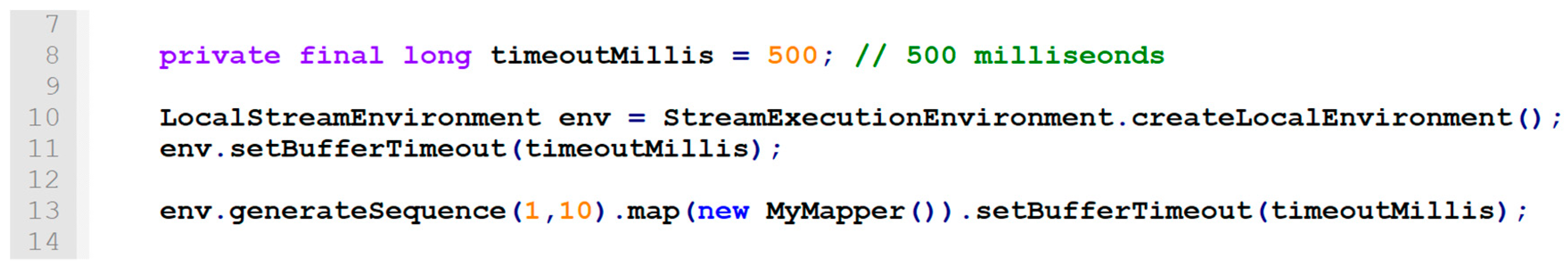
4.3. Dynamic maxOutOfOrderness and Task Tracker’s bufferingTimeout

Most frameworks have no capabilities that enable them to select the out-of-order ness of all incoming events at system runtime, and likewise, these systems often suffer from the static configuration of the buffering time-out. This absence of such features usually results in the breaching of the SLA agreements dealing with the reliable estimation of outcomes, guaranteed throughput (in case of throughput-intensive applications), some forms of manual end-to-end latency for specific systems (in case of response time-sensitive applications such as financial fraud detection, security systems etc.), and so on.

As opposed to the offered Flink framework, we propose an innovative framework model by making the maxOutOfOrderness and task tracker’s buffering timeout more flexible and dynamic at runtime, providing the system with a sense of control, and adaptable at runtime to any manually defined SLAs. The target values of the two are sent to, and maintained in every node, as follows:

4.3.1. Dynamic maxOutOfOrderness

The getCurrentWatermark procedure is used to get the current watermark of the data stream to keep track of the event and processing time of the system. In every iteration, the getCurrentWatermark() method in the run() method of the timestamp and watermark generator’s thread is invoked, our proposed system will call for the master whether the maxOutOfOrderness value was changed or otherwise and will go through with the selected path using the dynamic latency control mechanism accordingly. The proposed system uses a custom-based API to handle the runtime alteration of the out-of-orderness of events in the incoming workload following the procedure and guidelines of the Latency-Throughput control algorithm. In order to avoid the communication overhead from messaging, the communication with the master will be periodic or as necessary. If the maxOutOfOrderness has been altered, the system will change the local variable in the timestamp and watermark generator thread accordingly.

4.3.2. DYNAMIC bufferingTimeout

The connection manager of every node’s task manager sends a request to the master node about the buffer timeout value periodically. Should there have been any changes, then the connection manager will update its local buffer timeout values as needed, while the current ongoing buffer will contain all previous values before the update, and the system will provide the updated value for any generated buffers down the line. The recorded task manager’s value for the buffer timeout is the one changed through custom-based API of the proposed system following the rules and guidelines of the Latency-Throughput control algorithm as shown in Figure 10 and detailed in Section 4.2.

4.4. Target Latency Modes

We propose the following three modes of operations to achieve the target latency of the system: fully automated mode, semi-automated mode, and manual mode.

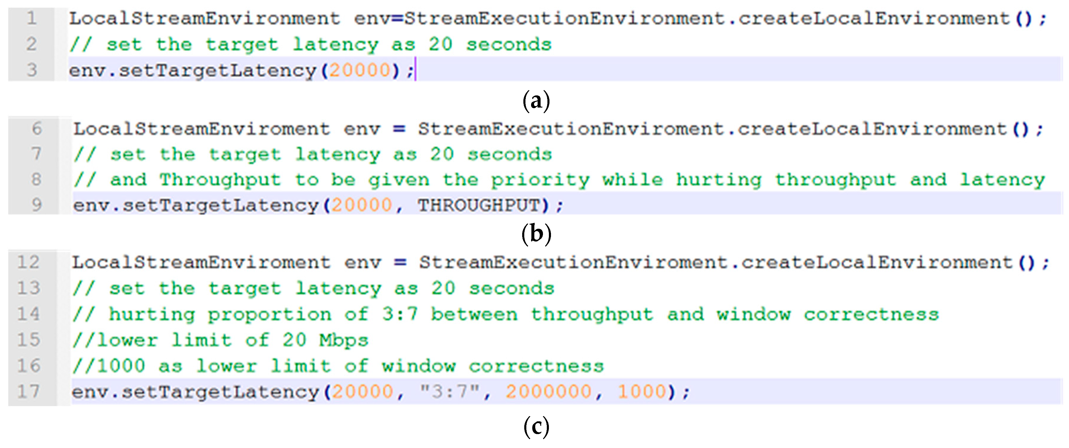
4.4.1. Fully Automated Mode: setTargetLatency(target latency value)

Fully automated mode in the proposed system will automatically provide a sub-optimized ratio between throughput and window correctness of any given workload based on the target latency provided by the user. Based on that, the modified module of the Job Manager will decide the tradeoff between throughput and window correctness, then enforce it at runtime. We utilize a machine learning algorithm which analyzes different workloads and improves the relations between latency, throughput, and window correctness while taking the workload into account. The workloads must be normalized, as the kind of workloads differ.

To elaborate, let us assume we set the target latency of the system to 20 seconds as shown in Figure 11a. Upon detection that the current latency of the system is overflowed 20 seconds by the Flink framework, it will find an optimized tradeoff between throughput and window correctness automatically, all the while factoring the nature of the workload into account.

4.4.2. Semi-Automated Mode: setTargetLatency(target Latency, priority of hurting throughput and window correctness)

In the semi-automated mode, users will establish the value for the target latency and prioritize which of the two, throughput or window correctness, must be sacrificed in a higher capacity, while calculating the sub-optimized solution for the tradeoff between both.

Again, to elaborate, let us assume a user has set the target latency of the system to 20 s and selected throughput as the defining factor over windowing correctness when one has to be chosen as shown in Figure 11b. After Flink determines that the current latency overflew 20 s, it will find an optimized tradeoff between throughput and correctness automatically with the intention of favoring throughput rather than correctness.

4.4.3. Manual Mode: setTargetLatency(target latency, hurting proportion between throughput and window correctness, low limit for throughput, low limit for window correctness)

For manual mode, the user will have to supply the required target latency, which affects the ratio between throughput and window correctness, providing a lower limit for affecting throughput for the sack of latency, and a lower limit for affecting window correctness, allowing the system to calculate the tradeoff between both.

To elaborate, suppose a user sets the target latency of the system to 20 s, resulting in a proportion of 3:7 between throughput and window correctness, low limit of 20 Mbps, and 1000 as the low limit of window correctness as in Figure 11c. After Flink detects that current latency overflew 20 s, it will hurt throughput and window correctness according to 3:7 proportion of throughput and correctness, while taking into account low bound for hurting throughput and the low limit value for hurting window correctness according to the given arguments. If the system cannot fulfill these conditions, it alerts the user about the situation.

In brief, all these operating modes i.e. fully automated mode, semi-automated mode, and manual mode are the variation of a core API function defined in our extension of the original open source framework called “setTargetLatency”. This function is called through the execution environment variable in order for the system to communicate with the system administrator. These functions allows administrators and users to define their SLAs and communicate it to the system in a seamless manner.

5. Evaluation

5.1. Workload Analysis

We use the real-life open-source dataset of German credit fraud data provided by Hamburg University for experimentation [17]. The dataset is chosen due to the reason that no specialized knowledge is required to understand the addressed application. Several changes were planted into the German Credit data to be found by the system and be verified if it can be found accordingly. The dataset contains two classes, as “good” and “bad” credits, and about 20 attributes of each and every person with a status of an existing checking account, credit history, amount, purpose, employment information, guarantors, properties, number of credit cards, and so on. For workload analysis purposes, we use three different classifiers, i.e., a naive Bayes classifier, multilayer perceptron (MLP), and sequential minimal optimization (SMO).

The naive Bayes classifier is a probabilistic classifier based on applying Bayes theorem [18] with strong or naïve independence assumptions between features. Numeric estimator precision values are chosen based on an analysis of the training data. Due to this reason, the classifier is not an updatable classifier and typically initiated with zero training instances. The updatable version is a naïve Bayes updatable classifier which uses the default precision of 0.1 for numeric attributes when called with zero training instances [19]. It is highly scalable, requiring a number of parameters linear in the number of features in a learning problem. Maximum-likelihood training, in this case, can be done through evaluating a closed-form expression, which takes linear time, rather than by complex and expensive iterative approximation as used for many other types of classifiers.

MLP is a class of feedforward artificial neural network, where each MLP consist of at least three layer nodes: an input layer, a hidden layer, and an output layer. Each node is a neuron, except for the input nodes and each neuron uses a nonlinear activation function. MLP utilizes backpropagation supervised learning technique for training [20]. It can distinguish non-linearly separable data due to its multiple layers and non-linear activation. Its network can be built by hand, created by an algorithm, or both. The network can also be modified and monitored during training time.

SMO is usually used for solving the quadratic programming problems that arise during the support vector machines training [21]. It can globally replace all the missing values and transforms nominal attributes into binary ones. It also normalizes all the attributes by default. In order to obtain proper probability estimates, an option that fits calibration models to the outputs of the support vector should be selected. The predicted probabilities are coupled using the pairwise coupling method [22].

We analyze the German credit fraud dataset using the above algorithms. The results are shown in Figure 12. The columns indicate correctly classified instances, incorrectly classified instances, Kappa statistic, mean absolute error, root mean squared error, relative absolute error, and root relative squared error accordingly. Naïve Bayes classifies the highest correct number of instances and with the lowest root relative error and root mean squared error. SMO has the lowest relative absolute error and means absolute error accordingly. The model building time is summarized in

Table 1. Algorithms model building time.

Algorithm	Model Building Time (s)
Naïve Bayes	5.3
Multilayer Perceptron	21.9
SMO	10.3

, showing that Naïve Bayes algorithm has the ability to model the scenario in the lowest time of the other two algorithms despite the number of tuples in the dataset. Naïve Bayes has a 5.2 s model building time, SMO has 10.3 s, and multilayer perceptron has a 21.19 s model building time. The resultant analysis of the workload is transferred to the Job Manager at runtime to be used by the decision process module for the system later on. We are currently working on the custom adaptor to make it happened and will be published with our upcoming research work.

5.2. System Experimentation

In

Table 2. Cluster configuration (adapted from [12]).

Hardware/Software	Configuration
Cluster	Amazon EMR cluster version 5.6.0
Nodes	M3.xlarge (8 vCPU, 15GB, 80 SSD)
No of Instances	3
Flink	Version 1.2.1
Ganglia	Version 3.7.2
Storage Services	Amazon S3

, we show our proposed system’s hardware and software configuration. We performed our experiments using the Amazon EMR (Elastic MapReduce) 5.6.0 with advanced options of selecting both Apache Flink and Ganglia as the main software to be installed, as well as the pre-configuration of the cluster formation and setup. We chose three m3.xlarge instances with eight vCPUs, 15 GiB memory, and an 80 GB SSD. Ganglia is primarily purposed to monitor the cluster and performance of each machine individually. We use the YARN cluster, with default parallelism of 8 as the base cluster for Flink jobs, to be executed to keep the application master up and running.

5.3. Performance Evaluation Experimentation

Firstly, we have found an interesting system effect; with the increase in buffer timeout, both the throughput and latency start to proportionately increase as well, thus proving that both throughput and latency are directly proportional to buffering timeout. This fact details that Flink operators first gather the records in their buffers, before passing them on to the next operator. By specifying the buffer timeout, we notify Flink’s runtime to empty the buffer after the stated time even if it is not full. A lower buffer timeout usually means lower latency, although at the expense of throughput as shown in Figure 13. For time-sensitive cases like fraud detection in financial applications or IT security, response time is critical; latencies higher than 30 ms usually lead to late detection of the problem, which defies the purpose of such applications. The latency boundaries show that both latency and throughput are inversely proportional to one another. We require a system that analyzes the workload and develops a potential ideal trade-off of the two.

The second group of tests reveals that window correctness (as with the increase of allowed lateness, the window correctness increases as well) alter the productivity of the application. This experiment is also done under the same EMR cluster configuration of three m3.xlarge instances of Amazon. The setup uses the streaming application to read parallel streams of events form Apache Kafka [23] and checks the validity of it, like token authentication, service interaction, and login authentication. We also design to push some false late elements (elements with timestamp t’ <= t) to prominence the window correctness problem, meaning that it is unrealistic to postulate a time through which all elements of a definite event timestamp should have happened, leading to late elements in the data stream to be picked up and process with the original data. We collect and analyze the average job execution time, with differing values of allowed lateness ranging from 0 to 30 as published in

Table 3. Job execution time with the varying value of allowed lateness.

Allowed Lateness (s)	Job Execution Time (s)
0	420
5	435
10	467
20	533
30	579

. The experiment shows that the window correctness of the results rises at the cost of total job execution time. Here the increase in the allowed lateness is consistent with the window correctness, i.e., as the allowed lateness increases, it increases the chances of the window to be correct and more accurate in its calculations. This is due to the effect that allowed lateness decreases the chances of elements for the specified window to be late, whereas the increase in the gap for the execution time is a result of an increased delay, causing the Kafka stream to heighten its queue time, altering the overall capabilities of our proposed system.

In an effort to emphasize our definition of latency, another set of experiments shows the event time and processing time latencies under the condition when the system is extremely overloaded. For this set of experiments, we overloaded the system with high input and disabled the system capability to readjust according to the workload to demonstrate the difference between event time latencies and processing time latencies, as shown in Figure 14. This experiment reveals that the processing time latency is significantly lower than the event time latency. The reason behind this phenomenon is that the system creates backpressure due to overloaded incoming workload and lowers the data processing rate to stabilize the end-to-end system latency. The backpressure problem has been addressed in our previous work using the optimized scheduling technique for stream processing [24] and will be discussed in details in our upcoming article. The event time latency keeps increasing as the input data stream waits in the queues while the system stabilizes the end-to-end latency.

Moreover, in this set of experiments, we elaborate the combined effect of our proposed system by designing an experiment to capture the performance of the system, utilizing a varying number of bytes of input data as shown in Figure 15. In the event that the volume of input data is less than expected, both the CASE-Flink and default Flink performance are similar. On the other hand, with the rise in the amount of data, CAS-Flink outshines the default Flink system without scaling out any cases to the EMR cluster. The progress of our system is that we have an algorithmic system in place for the extraction of the latency and throughput metrics within the cluster. At the current moment, there is no need to modify the Flink framework, and we intend to keep things that way, at least temporarily. Also, our workload analyzer is in place to be mounted into the system without significant changes and modification to the core system. We are currently working on the custom adaptor to be used to transfer the analysis results and calculated metrics to the Job Manager on the runtime so that the system would be able to make its decision module automatize based on the metrics received on the fly. We considered another set of experimentation with other major streaming engines like Spark, Storm, and Heron whose comparison is already done in several previous articles, including Spark vs. Flink vs. Storm [25], benchmarking streaming computation engines [26], and side-by-side comparison of streaming engines in [27]. If is for these reasons we design other experimentation instead of just comparing different streaming engines which have been previously handled by many researchers in the research community.

Moreover, in this set of experiments, we manually transfer the workload analysis results to the decision module to make the system more automated. The resultant behavior of the system is shown in Figure 16. It is clear from the figure that the default system has the highest latency in each case following by SMO based CAS-Flink, MLP based CAS-Flink, and naïve Bayes CAS-Flink with the minimum latency. The naïve Bayes-based CAS-Flink system is more promising and shows that with the increase in the incoming streaming data, the system is able to sub-optimally decrease the execution time of the application without the breach in the SLA agreement as well as without any adverse effect on the quality of service (QoS). The results shows that all the workload analysis based systems outperform the default system, this effect is due to the fact that with the overloading, the default system stabilizes its latency at higher value leading to the effect of the incoming stream of data to wait in the queues longer and causes SLA breach or reduction in QoS.

6. Related Research

The increasing relevance of streaming engines has resulted in a number of projects focused on exploiting parallelism in stream processing and scale-out. Apache S4 [28], Strom [5], and Flink [9] represent queries and programs as directed acyclic graphs (DAGs) with parallel operators. S4 schedules parallel instances of operators at the cost of being able to control such operators. Storm allows users to stipulate a parallelization level and supports stream partitioning based on key intervals, but it ignores states of operators and has minimal ability to scale at runtime. System S [29] from IBM supports intra-query parallelism through a fine-grained subscription model that has the ability to describe any and all stream connections. This system has no automated manager for the said mechanism. Hizrel [30] proposed a MatchRegex operator for System S to detect tuple pattern in parallel. This approach does not consider dynamic repartitioning and state is specific to automata-based pattern detection. Stromy [31] uses consistent hashing and a logical ring to accommodate new nodes upon scale out. It does not take congestion into account, while our proposed system does. Zeitler and Risch [32] proposed the parasplit operator for a partitioning stream statically based on a cost model, allowing for a customized stream splitting for the scalable execution of continuous queries over massive data streams. Instead, our take on this decides the parallelization level at runtime, based on performance metrics.

StreamCloud [33] constructs elasticity into Borealis Stream Processing Engine [34]. StreamCloud uses a query compiler to synthesize high-level queries into graphs of relational algebra operators. It uses hash-based parallelization, which is geared towards the semantics of joins and aggregates. It modifies the parallelism level through splitting queries into subqueries and uses rebalancing to adjust resource usage. Our proposed approach CASE-Flink reconfigures the out-of-orderness in the input events occurrences and buffering timeout while complying with user-defined SLA agreement. Backman et al. [35] partition and distribute operators across nodes within the stream processing system to reduce the amount of processing latency through load balancing according to the simulated estimation of latency. They achieve latency-minimization goals through parallelism model encouraged by latency-oriented operator scheduling policy coupled with the diversification of computing node responsibilities. In contrast, our method of the operator over the cluster nodes is done when needed to remove the processing bottlenecks and achieve low latency.

SEEP [36] proposed an elastic approach based on operators state management. It exposes internal operator state explicitly to the stream processing system through a set of state management primitives. Based on these primitives, it describes an integrated approach to dynamically scale and recover stateful operators through periodic checkpointing of externalized operator state by streaming processing systems and backed up to upstream VMs. It offers mechanisms to backup, restores, and partition operator’s states in order to achieve short recovery time. Auto-parallelization [37] addresses the profitability problem associated with automatic parallelization of general purpose distributed data stream processing applications. Their proposed solution can dynamically adjust the numbers of channels used to achieve high throughput and high resource utilization as well as handle partitioned stateful operators through run-time state migration. In contrast, our approach takes workload into account and adjusts the configuration of anticipated metrics at runtime to meet the SLA requirements.

Twitter’s Heron [38] improves Strom’s congestion handling mechanism by using back pressure. However, it fails to address the elasticity and reconfiguration of topologies specifically. Heinze et al. [39] proposed an online parameter optimization approach allowing the system to trade a monetary cost in exchange for the offered QoS. It focused on latency and policy, rather than throughput and mechanism. Reactive-Scaling [40] presents a flexible elastic strategy for enforcing constraints over latencies in a scalable streaming engine while minimizing resource footprints. Their queuing theoretic latency model provides a latency guarantee by tuning the task-wise level of parallelism in a fixed size cluster. It should be pointed out that our proposed mechanisms can be used as a black box within both systems [39,40].

7. Concluding Remarks and Future Directions

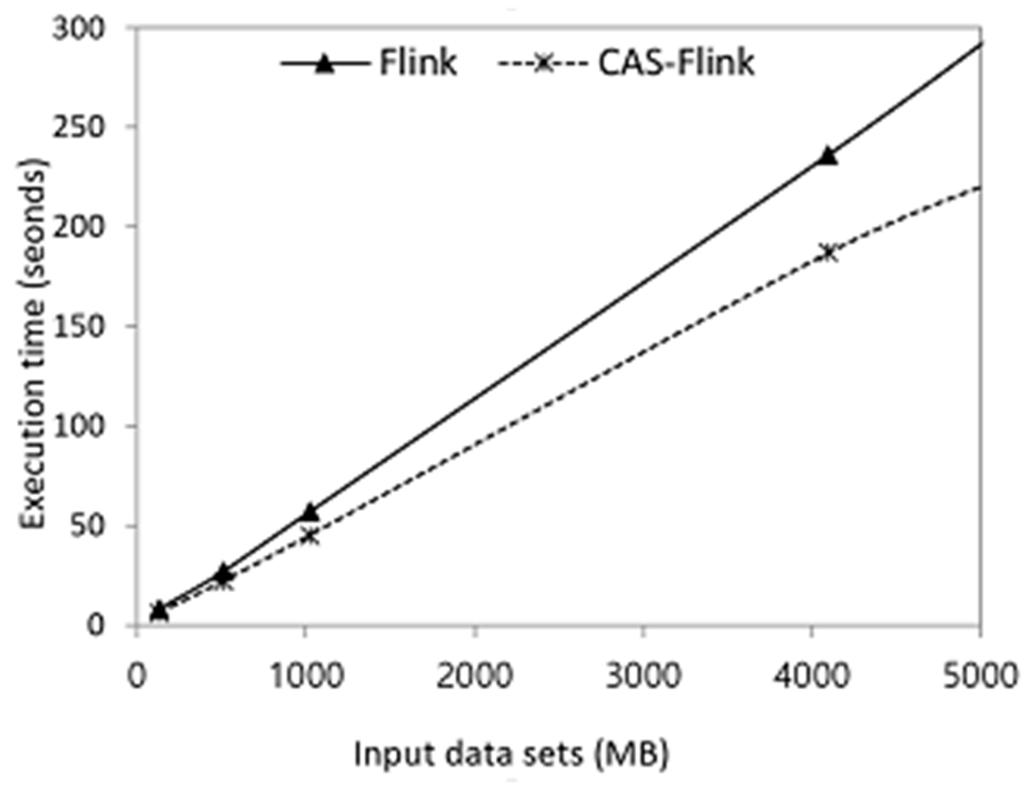
The growing popularity of the Flink framework is due to the wide range of use cases for this platform and its capability to handle both batch and streaming applications and data in a fault-tolerant and efficient way. As an evolving open source framework in the field of big data analytics and distributed computing, Apache Flink has the competency of processing distributed data streams in a reliable and real-time fashion. We proposed an efficient, adaptive watermarking and dynamic buffering timeout mechanism for Apache Flink. It is designed to increase the overall throughput by making the watermarks of the system adaptive based on the workload, while also providing a dynamically updated buffering timeout for every task tracker instantly, all the while maintaining the SLA based end-to-end latency of the system. The main focus of this work is on tuning the parameters of the system based on the incoming workloads and assesses whether a given workload will breach an SLA using output metrics including latency, throughput, and window correctness. Our experimental results show that CAS-Flink outperforms existing distributed stream processing engines.

We plan to investigate more efficient workload analysis methods like Markov Model, and Markov Hidden Model. We believe by introducing such models, and we will be able to fully automatize the system with the inclusion of topology refining scheme to the current model, which will lead the system to be more robust and load balanced within the limits of its SLA agreements and without hurting the QoS accordingly.

References

1. Mell, P.; Grance, T. The NIST Definition of Cloud Computing; National Institute of Standards & Technology: Gaithersburg, MD, USA, 2011; Volume 145, p. 7. [Google Scholar]
2. Demchenko, Y.; De Laat, C.; Membrey, P. Defining Architecture Components of the Big Data Ecosystem. In Proceedings of the 2014 International Conference on Collaboration Technologies and Systems (CTS), Minneapolis, MN, USA, 19–23 May 2014; pp. 104–112. [Google Scholar] [CrossRef]
3. Dean, J.; Ghemawat, S. MapReduce: Simplified data processing on large clusters. ACM Commun. 2008, 51, 107–113. [Google Scholar] [CrossRef]
4. White, T. Hadoop: The Definitive Guide, 3rd ed.; O’Reilly Media: Sebastopol, CA, USA, 2012; Volume 54, ISBN 978-1-4493-1152-0. [Google Scholar]
5. Toshniwal, A.; Taneja, S.; Shukla, A.; Ramasamy, K.; Patel, J.M.; Kulkarni, S.; Jackson, J.; Gade, K.; Fu, M.; Donham, J.; et al. Storm @ Twitter. In Proceedings of the 2014 ACM SIGMOD International Conference on Management of Data, Snowbird, UT, USA, 22–27 June 2014; pp. 147–156. [Google Scholar] [CrossRef]
6. Zaharia, M.; Das, T.; Li, H.; Hunter, T.; Shenker, S.; Stoica, I. Discretized Streams: Fault-Tolerant Streaming Computation at Scale. In Proceedings of the Twenty-Fourth ACM Symposium on Operating Systems Principles, Farminton, PA, USA, 3–6 November 2013; pp. 423–438. [Google Scholar] [CrossRef]
7. Feng, T.; Zhuang, Z.; Pan, Y.; Ramachandra, H. A Memory Capacity Model for High Performing Data-filtering Applications in Samza Framework. In Proceedings of the 2015 IEEE International Conference on Big Data, Santa Clara, CA, USA, 29 October–1 November 2015; pp. 2600–2605. [Google Scholar] [CrossRef]
8. Akidau, T.; Bradshaw, R.; Chambers, C.; Chernyak, S.; Fern, R.J.; Lax, R.; Mcveety, S.; Mills, D.; Perry, F.; Schmidt, E.; et al. The Dataflow Model: A Practical Approach to Balancing Correctness, Latency, and Cost in Massive-Scale, Unbounded, Out-of-Order Data Processing. In Proceedings of the 41st International Conference on Very Large Data Bases, Kohala Coast, HI, USA, 31 August–4 September 2015; pp. 1792–1803. [Google Scholar] [CrossRef]
9. Carbone, P.; Ewen, S. Apache Flink TM: Stream and Batch Processing in a Single Engine. In Bulletin of the IEEE Computer Society Technical Committee on Data Engineering; IEEE Computer Society: Washington, DC, USA, 2015; pp. 28–38. [Google Scholar]
10. Apache! ApacheTM Hadoop®! Available online: http://hadoop.apache.org/ (accessed on 31 December 2015).
11. Hummer, W.; Satzger, B.; Dustdar, S. Elastic stream processing in the cloud. Wiley Interdiscip. Rev. Data Min. Knowl. Discov. 2013, 3, 333–345. [Google Scholar] [CrossRef]
12. Hanif, M.; Yoon, H.; Jang, S.; Lee, C. An adaptive SLA-based data flow mechanism for stream processing engines. In Proceedings of the International Conference on Information and Communication Technology Convergence (ICTC), Jeju Island, Korea, 18–20 October 2017; pp. 81–86. [Google Scholar] [CrossRef]
13. Gee, S. Fraud and Fraud Detection: A Data Analytics Approach; John Wiley & Sons: New York, NY, USA, 2014; 355p. [Google Scholar]
14. Flink!, Job Scehudling Internals: Flink. Available online: https://ci.apache.org/projects/flink/flink-docs-release-1.3/internals/job_scheduling.html (accessed on 25 October 2018).
15. Miguel-alonso, T.L.J.; Lozano, J.A. A Review of Auto-scaling Techniques for Elastic Applications in Cloud Environments. J. Grid Comput. 2014, 12, 559–592. [Google Scholar] [CrossRef]
16. Calheiros, R.N.; Masoumi, E.; Ranjan, R.; Buyya, R. Workload Prediction Using ARIMA Model and Its Impact on Cloud Applications ’ QoS. IEEE Trans. Cloud Comput. 2015, 3, 449–458. [Google Scholar] [CrossRef]
17. Merz, C.J.; Murphy, P. Uci Repository of Machine Learning Databases. 1988. Available online: http://www.cs.uci.edu/mlearn/MLRepository.html (accessed on 12 December 2018).
18. Schulman, P. Bayes’ theorem—A review. Cardiol. Clin. 1984, 2, 319–328. [Google Scholar] [CrossRef]
19. John, G.H.; Langley, P. Estimating Continuous Distribution in Bayesian Classifiers. In Proceedings of the UAI’95 Eleventh Conference on Uncertainty in Artificial Intelligence, Montreal, QC, Canada, 18–20 August 1995; pp. 338–345. [Google Scholar]
20. Rumelhart, D.E.; Hinton, G.E.; Williams, R.J. Learning Internal Representations by Error Propagation. In Readings in Cognitive Science: A Perspective from Psychology and Artificial Intelligence; Elsevier: Amsterdam, The Netherlands, 2013; pp. 399–421. ISBN 1558600132. [Google Scholar]
21. Platt, J.C. Sequential minimal optimization: A fast algorithm for training support vector machines. Adv. Kernel Methods Support Vector Learn. 1998, 208, 1–21. [Google Scholar]
22. Quost, B.; Destercke, S. Classification by pairwise coupling of imprecise probabilities. Pattern Recognit. 2017. [Google Scholar] [CrossRef]
23. Wang, G.; Koshy, J.; Subramanian, S.; Paramasivam, K.; Zadeh, M.; Narkhede, N.; Rao, J.; Kreps, J.; Stein, J. Building a Replicated Logging System with Apache Kafka. In Proceedings of the VLDB Endowment, Kohala Coast, HI, USA, 31 August 2015; pp. 1654–1655. [Google Scholar] [CrossRef]
24. Yoon, H.; Lee, C. Optimized Stream Processing Task Scheduling in Flink. In Proceedings of the Korea Computer Congress, Jeju, Korea, 18–20 June 2017. [Google Scholar]
25. Evans, B. Spark VS flink VS Storm. YAHOO! Eng. 2015. Available online: https://www.mendeley.com/catalogue/spark-vs-flink-vs-storm/ (accessed on 12 March 2019).
26. Chintapalli, S.; Dagit, D.; Evans, B.; Farivar, R.; Graves, T.; Holderbaugh, M.; Liu, Z.; Nusbaum, K.; Patil, K.; Peng, B.J.; et al. Benchmarking streaming computation engines: Storm, flink and spark streaming. In Proceedings of the 2016 IEEE International Parallel and Distributed Processing Symposium Workshops (IPDPSW), Chicago, IL, USA, 23–26 May 2016; pp. 1789–1792. [Google Scholar]
27. Huynh, X. Storm vs. Spark Streaming: Side-by-side comparison. Xinh Tech. 2014. Available online: https://www.mendeley.com/catalogue/storm-vs-spark-streaming-sidebyside-comparison/ (accessed on 12 March 2019).
28. Neumeyer, L.; Robbins, B.; Nair, A.; Kesari, A. S4: Distributed stream computing platform. In Proceedings of the IEEE International Conference on Data Mining, ICDM, Sydney, NSW, Australia, 13 December 2010; pp. 170–177. [Google Scholar] [CrossRef]
29. Amini, L.; Andrade, H.; Bhagwan, R.; Eskesen, F.; King, R.; Selo, P.; Park, Y.; Venkatramani, C. SPC: A Distributed, Scalable Platform for Data Mining. In Proceedings of the 4th International Workshop on Data Mining Standards, Services and Platforms, Philadelphia, PA, USA, 20 August 2006; pp. 27–37. [Google Scholar] [CrossRef]
30. Hirzel, M. Partition and Compose: Parallel Complex Event Processing. In Proceedings of the International Conference on DEBS, Berling, Germany, 16–20 July 2012; pp. 191–200. [Google Scholar] [CrossRef]
31. Loesing, S.; Hentschel, M.; Kraska, T.; Kossmann, D. Stormy: An elastic and highly available streaming service in the cloud. In Proceedings of the 2012 Jt. EDBT/ICDT Work. EDBT-ICDT ’12, Berlin, Germany, 30 March 2012; pp. 55–60. [Google Scholar] [CrossRef]
32. Zeitler, E.; Risch, T. Massive scale-out of expensive continuous queries. In Proceedings of the 36th International Conference on VLDB Endow, Singapore, 13–17 September 2011. [Google Scholar]
33. Gulisano, V.; Jiménez-Peris, R.; Patiño-Martinez, M.; Soriente, C.; Valduriez, P. StreamCloud: An elastic and scalable data streaming system. IEEE Trans. Parallel Distrib. Syst. 2012, 2351–2365. [Google Scholar] [CrossRef]
34. Abadi, D.J.; Ahmad, Y.; Balazinska, M.; Çetintemel, U.; Cherniack, M.; Hwang, J.-H.; Lindner, W.; Maskey, A.; Rasin, A.; Ryvkina, E.; et al. The Aurora and Borealis Stream Processing Engines. In Data Stream Management; Springer: Berlin/Heidelberg, Geramny, 2016; pp. 337–359. [Google Scholar]
35. Backman, N.; Fonseca, R.; Çetintemel, U. Managing parallelism for stream processing in the cloud. In Proceedings of the 1st International Workshop on Hot Topics in Cloud Data Processing, Bern, Switzerland, 10 April 2012; pp. 1–5. [Google Scholar] [CrossRef]
36. Fernandez, R.C. Integrating scale out and fault tolerance in stream processing using operator state management. In Proceedings of the 2013 ACM SIGMOD International Conference on Management of Data, New York, NY, USA, 23–28 June 2013; pp. 1447–1463. [Google Scholar] [CrossRef]
37. Gedik, B.; Schneider, S.; Hirzel, M.; Wu, K.L. Elastic scaling for data stream processing. IEEE Trans. Parallel Distrib. Syst. 2014, 25, 449–458. [Google Scholar] [CrossRef]
38. Kulkarni, S.; Bhagat, N.; Fu, M.; Kedigehalli, V.; Kellogg, C.; Mittal, S.; Patel, J.M.; Ramasamy, K.; Taneja, S. Twitter Heron: Stream Processing at Scale. In Proceedings of the 2015 ACM SIGMOD International Conference on Management of Data, Melbourne, Victoria, Australia, 31 May–4 June 2015; pp. 239–250. [Google Scholar] [CrossRef]
39. Heinze, T.; Roediger, L.; Meister, A.; Ji, Y.; Jerzak, Z.; Fetzer, C. Online Parameter Optimization for Elastic Data Stream Processing. In Proceedings of the Sixth ACM Symposium on Cloud Computing, Kohala Coast, HI, USA, 27–29 August 2015; pp. 276–287. [Google Scholar] [CrossRef]
40. Lohrmann, B.; Janacik, P.; Kao, O. Elastic Stream Processing with Latency Guarantees. In Proceedings of the International Conference on Distributed Computing Systems, Columbus, OH, USA, 29 June–2 July 2015; pp. 399–410. [Google Scholar] [CrossRef]
Figure 1. Fraud detection and prevention system based on Amazon and Apache Flink.
Applsci 09 01045 g001
Figure 2. Apache Flink architecture: Running and dataflow creation of a Flink program on the Flink system, and distribution of the operators to the available slots on each Task Tracker by the Job Manager through the Actor system.
Applsci 09 01045 g002
Figure 3. Distribution of operators in a distributed stream processing framework (adapted from [12]).
Applsci 09 01045 g003
Figure 4. Generating watermark based on the maximum out of orderness of six seconds for the data stream.
Applsci 09 01045 g004
Figure 5. Generating the sequence and transferring it between machines using 500 ms as buffer timeout.
Applsci 09 01045 g005
Figure 6. Subtask concept based on the condensed and parallelized view of the streaming dataflow.
Applsci 09 01045 g006
Figure 7. Different notions of time in a stream processing lifetime.
Applsci 09 01045 g007
Figure 8. Late elements detection through the watermarking mechanism.
Applsci 09 01045 g008
Figure 9. Proposed system architecture: Event gathering systems collect the data, pipelining it to the data broker for validation, then passing it onto the workload analyzer, which finally passes the obtained results onto the Job Manager through workload prediction module (adapted from [12]).
Applsci 09 01045 g009
Figure 10. Dynamic latency control mechanism: Using the expected metrics, this mechanism controls the system’s latency based on the established SLA agreements.
Applsci 09 01045 g010
Figure 11. (a) Fully automated mode example: Setting latency to 20 s according to SLA agreement. (b) Semi-automated mode example: Setting latency to 20 s and prioritizing throughput over latency according to SLA agreement. (c) Manual mode example: Setting latency to 20 s, ratio of 3:7 between throughput and window correctness, threshold of throughput to 20 MB, and threshold of window correctness to 1000 according to the SLA agreement.
Applsci 09 01045 g011
Figure 12. Workload analysis algorithms: Naïve Bayes, multilayer perceptron, and SMO comparisons based on correctly classified instances, incorrectly classified instances, Kappa statistic, mean absolute error, root mean squared error, relative absolute error, and root relative squared error.
Applsci 09 01045 g012
Figure 13. Throughput-latency tradeoff using varying task manager’s buffer timeout values (adapted from [12]).
Applsci 09 01045 g013
Figure 14. Event time vs. processing time latencies under conditions where the system is extremely overloaded with the incoming workload.
Applsci 09 01045 g014
Figure 15. Flink vs. CAS-Flink: The measured performance of Flink vs. CAS-Flink, utilizing a varying volume of input datasets (adapted from [12]).
Applsci 09 01045 g015
Figure 16. Application level performance evaluation of the system based on different workload analysis modules.
Applsci 09 01045 g016