Abstract
Although industrial robots are widely used in production automation, their applications in machining have been limited because of the structural vibrations induced by periodic cutting forces. Since the dynamic characteristics of an industrial robot depends on its configuration, the responses of the robot structure to the cutting forces are affected by how the workpiece is placed within the workspace of the robot. This paper presents a method for workpiece pose optimization for a robotic milling system to improve the quasi-static performance during machining. Since the milling forces are time-varying due to the characteristics of the multi-tooth and discontinuity of milling, these forces can excite vibrations inside the robot structure. To address this issue, a structural dynamics model is established for industrial robots, considering their joint flexibility, and a milling force formulation is incorporated into the robot dynamics model to investigate the forced vibrations of the flexible joints. Then, the quasi-static performance of the robotic machining system is evaluated by the vibration-induced offset of the cutter tool that is mounted on the end-effector. Finally, an optimization approach is given for the workpiece pose to minimize the cutter tool offset under the periodic milling force. A numerical simulation demonstrates that the optimal workpiece pose can significantly reduce the overall tool offset during machining and can lower the variation of the tool offset along the milling path.
1. Introduction
Due to their flexibility, efficiency, and reliability, industrial robots have played an important role in production automation for a wide spectrum of applications including welding, painting, assembly, packaging, and material handling [1]. Recently, these machines have also been proposed for more complex tasks with a large dynamic loading such as machining [2], and these robotic applications require a high positioning accuracy and involve large time-varying loading during the processes. A few examples are the European projects HEPHESTOS and COMET that were launched to develop innovative robotic machining systems for small-batch production [3,4] and Boeing’s initiative that aimed at using robots to automate drilling and percussive riveting processes in aircraft assembly [5]. On the other hand, the challenges for these robotic applications have also been highlighted in literature due to the inherent disadvantages of industrial robots compared with machine tools, such as having a low positioning accuracy and being prone to vibrations [2].
With the development of modern metrology techniques such as laser tracking [6,7] and photogrammetry-based measurement [8,9], the robotic positioning accuracy can be improved by kinematic parameter calibration [10,11,12] and positioning error compensation [7,8,13,14,15,16]. For example, Andres et al. [12] developed a calibration method to estimate the external joint configuration parameters using a laser displacement sensor. Morris et al. [16] developed a kinematic model for a robot arm through a coordinate measuring machine (CMM), and experimental measurements at some robot poses were taken using the CMM. However, industrial robots still face issues due to structural vibrations for these applications, and the resulting influence is difficult to eliminate by metrology techniques.
Robotic machining involves dynamic loading in a way that the magnitudes and directions of the force and torque acting on the robot dramatically change with time during machining. The resulting forced vibrations of the robot structure lead to much more complicated dynamics behaviors than many other robotic tasks such as pick-and-place and welding where static or very low contact forces act on the robot. First, the forced vibrations of the robot can seriously affect the process, for example, by decreasing the efficiency [17], damaging the surface quality [18], causing tool misalignment [19], and reducing the fatigue lives of the tool and the robot to a great extent [20,21]. Second, not only static but also inertial forces are important for these applications. Furthermore, the interaction between the machining forces and the robot vibrations can even cause instability to the robotic machining system [22,23] if some machining parameters such as spindle speed and feed rate are not selected properly [24,25]. All these works have shed some light on the complexity of structural dynamics of robotic machining.
Several approaches have been proposed to improve the robotic machining quality for a specific task considering the forced vibrations caused by machining. Vosniakos et al. [26] used two genetic algorithms to find the region with the best manipulability and the lowest joint torque in the robot workspace. Baglioni et al. [27] developed a parametric modeling procedure that can correctly simulate the robot dynamics behavior. Klimchik et al. [28] modeled the interaction between the milling tool and the workpiece and proposed a method for compensating the compliance errors based on a nonlinear stiffness model. Kaldestad et al. [29,30] adjusted the tool path to counteract the tool deflections during the milling operations after estimating the tool force and robot joint stiffness. Kubela et al. [31] proposed an online method for compensating the backlash errors induced by the drive reversion. Cordes et al. [32] proposed a new joint space model that combined the joint stiffness and the reversal error and then used the model to compensate the milling path deviation. Shi et al. [33] proposed a prediction model that could estimate the stable and unstable zones of milling process.
In a robotic machining system, the workpiece is usually clamped on a work table and must be placed within the work space of the robot. The configuration of the robot and the cutting force acting on it during machining are dependent upon the pose of the workpiece relative to the robot. It has been found that the natural frequencies of a robot strongly depend on its configuration [34] and that the robot stiffness varies significantly in different directions [35,36] and can be improved by optimizing the robot configuration for a given pick-and-place task [36,37,38], which implies that the vibration characteristics of robotic machining are affected by how the workpiece is placed with respect to the robot. For example, the robot stiffness is considered in Reference [37] for the optimization of the redundant degrees of freedom to minimize the displacement of the cutting tool under static force. In this paper, the forced vibrations of the robot are considered and the optimization goal is to minimize the overall steady-state offset amplitude of the cutting tool under the time-varying cutting force during the milling process. To this end, a structural dynamics model is established for industrial robots considering their joint flexibility, and a milling force formulation is incorporated into the robot dynamics model to investigate the forced vibrations of the flexible joints. Then, the quasi-static performance of the robotic machining system is evaluated by the vibration-induced offset of the cutter tool that is mounted on the end-effector. The performance is quasi-static because the effect of the robot’s deformation on the milling force is neglected. Finally, an optimization approach is given for the workpiece pose to minimize the cutter tool offset under the periodic milling force.
The next three sections of this work are organized as follows. Section 2 describes the robotic milling system and the problem statement. Section 3 presents the theoretical modeling, including the robot dynamics model, the milling force model, and the optimization approach for the workpiece pose. A numerical simulation study is given in Section 4.
2. System Description and Problem Statement
As shown in Figure 1, a robotic machining system for milling is being developed. The system is composed of a Kuka KR 300-2 PA robot, a cylindrical helical end milling cutter mounted the robot end-effector, a work table located within the robot workspace, a modular fixture placed on the work table, and a workpiece to be machined. Both the work table and the fixture have pin holes for positioning reference and bolt holes for fastening, and the workpiece is fixed on the fixture. In addition, the inclination angle θp between the fixture and the work table can be adjusted. As a result, the pose of the workpiece relative to the robot can be represented by the position of the fixture on the work table denoted by xp and yp and the inclination angle θp as displayed in Figure 1.
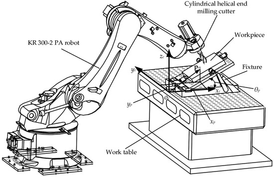
Figure 1.
The robotic milling system under study.
During the milling operation, the robot is subjected to periodic milling forces due to the intermittence of the cutter teeth. Since the machining operations can excite vibrations inside the robot structure, it is necessary to guarantee that the offset of the cutter tool maintains certain tolerances during the milling operation. In other words, the robot must be able to the hold the cutter tool firmly under the periodic milling forces. The machining forces can be changed by adjusting the machining parameters like the spindle speed and the feed rate; however, the adjustment of these parameters is constrained by many other factors such as the process efficiency requirement and the capability of the spindle and the robot. On the other hand, as mentioned above, the vibration characteristics of the system are also influenced by the workpiece pose relative to the robot, and the workpiece pose can be adjusted relatively easily. Then, the problem under study can be defined given the required milling tasks and milling parameters to find the optimal workpiece pose relative to the robot that minimizes the cutter tool offset under the periodic milling forces.
3. Theoretical Modeling
3.1. Dynamic Model of Robot
We first establish a structural dynamics model for the industrial robot to analyze the vibration characteristics. For this purpose, an n-DOF industrial robot with n links and n rotary joints is illustrated in Figure 2. A cutter tool is mounted on the robot end-effector. The local body-fixed coordinate systems {oi_xiyizi} (i = 1, 2,…,n) and the tool coordinate system {ot_xtytzt} are established at each joint and at the cutter tool tip, respectively. The position vector of the ith joint and the origin of tool coordinate system in the inertial coordinate system {o_xyz} are denoted by Pi and Pt respectively. During the milling operation, the cutter is subjected to an external machining force FE.
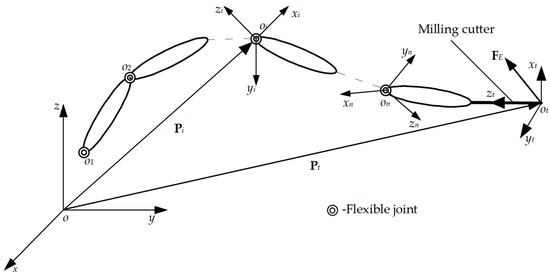
Figure 2.
The kinematic scheme.
For industrial robots, the main source of deformation is joint flexibility [1,39]. Thus, to simplify the robot model, we assume that all the links are rigid and that all the joints are equivalent to linear elastic torsion springs. If the joint angles for a given configuration are denoted as q = (q1, q2, …, qn)T, then the dynamic model of the stationary robot under forced vibrations in this configuration can be written as
where M represents the n × n symmetric generalized mass matrix, K is the n × n diagonal stiffness matrix with its diagonal entries equal to the torsional stiffness of the corresponding joints, and C is a damping matrix. Both K and C are defined in the joint space. Vector Δq is the perturbations in the joint angles from an equilibrium configuration and represents the joint deflections. The 3 × n linear velocity Jacobian matrix Jv represents the mapping from the joint rates to the velocity of the tool tip such that v = Jv, in which v is the linear velocity of tool tip written in the inertial coordinate system and is the joint rates. Matrices M and Jv depend on the robot configuration, and the force FE depends on the specific machining task.
The dynamic model described as Equation (1) is a linear time invariant system. Force FE can be considered as the external input, and Δq is the output response of the robot. In addition, if the joint deflection is small, the linear displacement of tool tip offset can be written as
Thus, once the joint deflection is obtained, the offset of the cutter tool caused by the robot vibration can be calculated through Equation (2), which can be used to evaluate the quasi-static performance of the robotic machining system under a specific machining force.
3.2. Milling Force Model
A cutting force model for cylindrical helical end milling is incorporated into the equation of motion of the robot to obtain the force vector FE, without considering the regenerative effect and the effect of the dynamic response of the robot on the cutting force [40,41]. In our system, up milling is chosen due to the concern with a backlash of the system. The readers are referred to Reference [42] for more detail about the cutting force modeling of down milling, which is similar in principle to that of up milling. In this cutting force model, the instantaneous cutting forces are assumed to be proportional to the area of contact between the flute and the workpiece [43]. Then, a mathematical model of the instantaneous milling force can be constructed by calculating the uncut chip thickness in a certain time. Then, the change of the cutter edge length during milling is analyzed to obtain the continuous milling force in the whole period. Figure 3 shows the geometric size and force condition of a single cutting edge of the cylindrical helical end mill. The tool coordinate system {ot_xtytzt} (also see Figure 2) is established as follows. The origin is at the center of the milling cutter tool tip, the zt axis is along the centerline of the milling cutter, the xt axis is along the direction of feed rate, and the yt axis is determined from the right-hand rule. N represents the number of milling teeth; β and R represent the helical angle and the radius of the cutter, respectively; and ap and ae represent the axial and radial depth of cut, respectively.
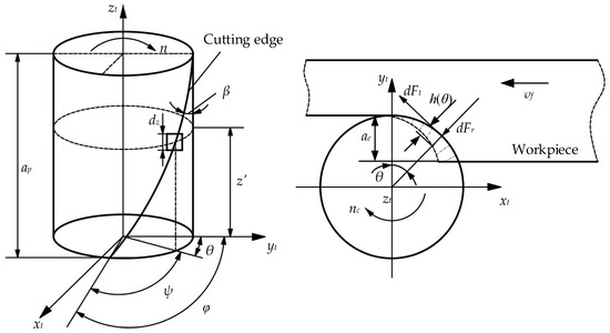
Figure 3.
The instantaneous milling force modeling.
Due to the existence of the helix angle of the cutter tool, the axial height of cutter teeth varies with the cutting thickness. Therefore, a microelement method is used to model a single cutter tooth. First, the cutter edge is discretized into numerous cutting-edge elements along the zt axis direction, and the height of each axial element is denoted as dz. φ represents the projection angle of the entire cutting edge in the xtotyt plane, and this projection angle is denoted as ψ when the axial height reaches z′. Then we have the following equations [42,43,44]:
where nc represents the spindle speed with a unit of rpm and t represents time. The cutting-edge angle θ between the microelement with an axial height of z′ and the yt axis can be calculated as
The determination of the cutting forces requires the area of contact between the end mill and the workpiece. For an axial element of thickness dz, this is equivalent to requiring the uncut chip thickness h. The uncut chip thickness h with an axial height of z′ can be approximately expressed as
where ft = vf/(nN) represents the feed per tooth and vf represents the feed rate. Because dz is very small, the area of contact with a height of dz between the flute and the workpiece at time t can be approximately equal to h(θ)dz. Then, we can calculate the elemental cutting force at this moment. Next, the force generated by this cutting tooth can be obtained by adding up all the elemental cutting forces. This is a definite integral problem, and we can get the result by integrating the axial height numerically. The upper and lower limits of integration can be obtained from the height of the cutting tooth involved during milling. In addition, there can be multiple cutting teeth involved in the cutting at time t. Then, we need to add up the forces from all the cutting teeth involved in the cutting to obtain the overall cutting force. The milling force is periodic because of the intermittence of the cutter teeth. The axial milling force along the zt axis can be neglected, since it is typically much smaller than the tangential and radial forces and has small contributions to the bending moment acting on the cutter tool. The detailed expressions for the tangential and radial milling forces are elaborated in thte Appendix A.
3.3. Steady-State Response and Optimization Method
Since the robot drives the tool to move slowly along the milling path, we can use the steady-state response of the cutter tool offset to evaluate the quasi-static performance of robotic milling in a given position. The cutter tool offset can be solved from Equations (1) and (2) in the time domain if the external forces are given. For a specific milling task, we select np points along the path and obtain the amplitudes di (i = 1, 2, …, np) of the steady-state responses of the cutter tool offset at these points. The steady-state response amplitudes di can also be obtained from Equation (1). Then, we calculate the mean value of all these amplitudes dm to quantify the overall quasi-static performance for this task. Then we have the following Equation:
If a local coordinate system {ow_xwywzw} is established on the workpiece, the position vectors pmi (i = 1, 2,…,np) of the selected points and the milling forces FEi (I = 1, 2,…, np) exerted on the cutter at these points in the inertial coordinate system can be expressed as
where pc and pw represent the position vectors of the work table and workpiece coordinate systems respectively and both vectors are written in the inertial coordinate system. In particular, vector pw can be obtained by xp and yp as pw = [xp, yp, zw]T in which zw is a constant and represents the height of the origin of workpiece coordinate system ow. Vectors pni (i = 1, 2,…,np) represent the position vectors of the selected points in the inertial coordinate system and can be calculated as pn = Rwz(θp)p’ni in which p’ni are the position vectors of the selected points in the workpiece coordinate system and Rwz(θp) represents the rotation matrix from the workpiece coordinate system to the inertial coordinate system. Vector F’ represents the cutting force in the tool coordinate system and can be obtained with the cutting force model presented in Section 3.2, and the 3 × 3 matrices Rni (i = 1, 2…np) represent the rotation matrices from the tool coordinate system of the selected points to the inertial coordinate system. Now, the process to calculate dm is illustrated in Figure 4.
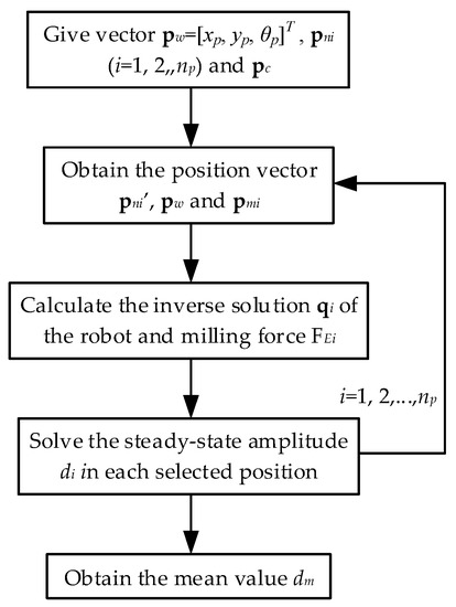
Figure 4.
The calculation flow chart of dm.
The workpiece has three degrees of freedom relative to the work table in this robotic milling system, which can be denoted by a parameter vector p = [xp, yp, θp]T. Then we aim at minimizing the mean value of the amplitudes of the cutter tool offset along the machining path by adjusting these parameters. The optimization problem can be expressed as
where dm is computed with the steps described in Figure 4. Once this optimization problem is solved, we find the optimal pose of the workpiece relative to the robot for the milling.
4. Numerical Simulation
4.1. System Parameters
In this simulation analysis, we only consider the flexibility of the first three joints of the robot because the moment arms of the cutting force about the last three joints are much shorter than those about the first three joints. The aforementioned coordinate systems in this simulation are described as follows. The inertial coordinate system {o_xyz} and the local coordinate systems {oi_xiyizi} (i = 1, 2, 3) of the robot are established as shown in Figure 5a. The inertial coordinate system is located at the base of the robot with the positive z-axis vertically upward and the y-axis perpendicular to the plane containing the second and third links. The zi-axis of the local coordinate systems are along the rotation directions of the corresponding joints; the axis x1 is parallel to the axis x when the robot is stationary, and the x2 and x3 axes are along the link length directions. The directions of the other reference axes of {oi_xiyizi} (i = 1, 2, 3) are determined from the right-hand rule. The local coordinate system of the work table {oc_xcyczc} is established at the middle position near the robot, with the xc and zc axes parallel to the x and z axes respectively and the yc axis is determined from the right-hand rule. The workpiece and the milling path are shown in Figure 5b. The workpiece coordinate system {ow_xwywzw} is established at the bottom of the workpiece, with the xw and yw axes parallel to the length and width and also parallel to the xc and yc axes respectively and the zw axis is determined from the right-hand rule.
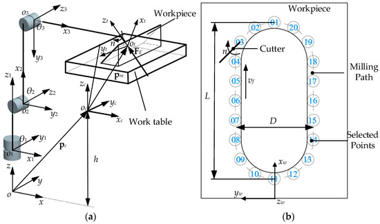
Figure 5.
The reference robotic milling system in the simulation: (a) The reference coordinate systems of the robot and work table and (b) the model of the workpiece and the milling groove.
The geometric, inertial, and structural parameters of the robot are described as follows. The link length vectors of o1o2, o2o3, and o3ot can be written in local coordinate systems of robot as I12 = [0, 0, l1]T, I23 = [l2, 0, 0]T, and I12 = [l3, 0, 0]T, where the link lengths are l1 = 0.2 m and l2 = l3 = 0.8 m. The masses, position vectors of the centers of gravity (CG), and inertia tensors of the links are listed in Table 1. Note that these vectors and tensors are written in the corresponding local coordinate systems. The torsional stiffnesses and damping of the three joints can be obtained by a stiffness identification experiment [45,46]. However, our system is still being built, and thus, the joint stiffness values available for a robot with similar payload and size are adopted, i.e., k1 = 2.4 × 10⁵ Nm/rad and k2 = k3 = 105 Nm/rad. A damping ratio ξ of 0.06 is used to compute the damping matrix based on the modal test data for industrial robots given in Reference [46]. Then, the ranges of the joint angles are θ1 є [−π, π], θ2 є [−π/2, π/2], and θ3 є [−π/3, π/3].

Table 1.
The inertial properties of the links.
The geometric parameters of the work table and the workpiece are described as follows. The position vector of the origin of the work table coordinate system oc are written as pc= [px, py, pz]T, where px, py, and pz are equal to 0.6 m, 0 m, and 0.5 m respectively. The length, width, and height of the work table are 1.16 m, 0.8 m, and 0.5 m, respectively, and the inclination angle of the fixture θp can change from 0 to π/3. The length L and width D of the milling path are 0.16 m and 0.08 m, respectively. We select 20 intermediate points uniformly distributed along the milling groove. The position vector of point 1 in the coordinate system {ow_xwywzw} is pn1 = [nx1, ny1, nz1]T, where nx1 = 0.12 m, ny1 = 0 m and nz1 = 0 m. The position vectors of the rest points can be calculated along the path.
The parameters for the cutter tool are described below. The teeth number and helical angle of the milling cutter are 2 and π/3 in this simulation. The diameter of the tool is 0.024 m, and the material of the tool and workpiece are uncoated tungsten carbide and aluminum alloy, respectively. The axial cutting depth and radial cutting depth are 0.002 m and 0.004 m, respectively, and the feed per tooth ft is 0.00012 m. The coefficient parameters kt1 and kt2 for calculating the cutting force (see Appendix A) are experimentally determined as 387 and 0.0018, respectively. Similarly, parameters b1 and b2 are determined as −0.327 and −0.224, respectively [43]. The readers are referred to the Appendix A for more information about these cutting force parameters.
4.2. Milling Force and Mean Value of Tool Offset
According to the milling parameters given in Section 4.1, we first obtain the milling force and its Fast Fourier Transform (FFT), as shown in Figure 6, when the speed n is equal to 1000 rpm. We can see that this spindle speed leads to a frequency of 33.33 Hz for the cutting force with two teeth.
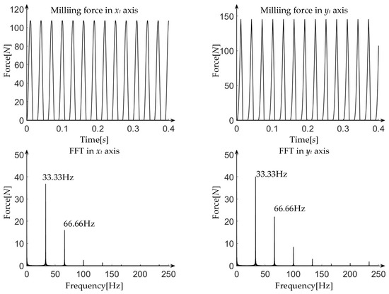
Figure 6.
The milling force and its Fast Fourier Transform (FFT).
In this simulation, we use the lsim function in MATLAB to compute the time-domain response of the joint deflections Δq under the periodic milling force from Equation (1). Then, the cutter tool offset can be obtained from Equation (2) for every point along the tool path.
Figure 7 shows the mean value of the tool offset amplitudes dm with different xp, yp, and θp and the variation of dm in the xpyp plane with different θp. The following observations can be found. In Figure 7a, when yp is equal to 0 m and 0.25 m, the deflection of joint 3 plays a major role when xp is between 0 m and 0.2 m. When xp increases, the torque acting on joint 3 due to the x component of the cutting force decreases. When xp is between 0.2 m and 0.6 m, the deformation of joint 1 plays a major role, and the torque acting on joint 1 due to the y component of the cutting force increases with the increase of xp. When yp is equal to 0.5 m, the deformation of joint 1 plays a major role; therefore, we see that dm increases when xp increases. In Figure 7b, it is seen that dm is asymmetrical about the oxz plane because the cutting forces are in opposite directions in every two symmetrical positions about the oxz plane along the milling groove. Figure 7c shows that dm increases when the inclination angle θp increases. This is likely because the z component of milling force and the resulting torques on joints 2 and 3 increase as the angle θp increases. Similarly, we find in Figure 7d that as angle θp increases, dm becomes larger. In addition, it can be seen from Figure 7d that when θp remains unchanged, dm decreases as the workpiece is placed closer to the robot. In particular, when vector p is equal to [0.6 m, 0.5 m, π/3]T and [0.6 m, −0.5 m, π/3]T, dm dramatically increases since the natural frequencies of the robot along the milling path with these workpiece poses are close to twice that of the milling force frequency (66.7 Hz).
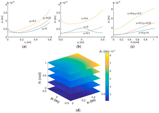
Figure 7.
dm with the different workpiece poses p: (a) The curves of dm change with xp when θp = 0 and yp = 0 m, 0.25 m, and 0.5 m; (b) the curves of dm change with yp when θp = 0 and xp = 0 m, 0.3 m, and 0.6 m; and (c) the curves of dm change θp when [xp, yp] = [0,0] m, [0.3, 0.25] m, and [0.6, 0.5] m. (d) The variation of dm in the xpyp plane when θp is equal to 0, π/12 rad, π/6 rad, and π/3 rad.
4.3. Optimization Results
In this section, the workpiece pose is optimized to minimize the mean value of the steady-state amplitudes of the cutting tool offset dm along the milling path defined in Figure 5b. Accordingly, the optimization problem in Equation (8) can be rewritten for this task as below:
To capture the possible coupling between the three optimization variables, a global optimization algorithm is used for solving the problem. The algorithm utilized here, called optQuest/NLP or OQNLP [47], is designed to find the global optima for pure and mixed integer nonlinear problems with multiple constraints and variables, where all the objective functions are differentiable with respect to the continuous variables. The optimization results and the other selected five sets of dates are listed for comparison in Table 2. The curves in Figure 8 show the steady-state amplitudes of the tool offset in the selected positions along the milling path with different workpiece poses p. We can find that dm introduced in Section 3.3 is strongly influenced by the workpiece pose. In addition, when the workpiece pose remains unchanged, dm can vary greatly at different points along the milling path. The optimal workpiece pose is obtained as p = [0, −0.46, 0]T, which gives the smallest average tool offset amplitude dm of about 0.22 × 10⁻³ m. Also, the tool offset changes relatively smoothly in different positions along the path compared with the variations with other workpiece pose parameters. dmi represents the dm at the position of the ith workpiece position.
Table 2.
dmi with different places of workpiece. * represents the set of result as the optimal workpiece pose.
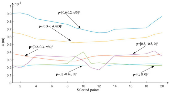
Figure 8.
di with different workpiece poses along the milling groove.
5. Conclusions
Structural vibration induced by periodic machining force is one of the main limitations for the application of industrial robots in machining. This paper presents a method for workpiece pose optimization for robotic milling to improve the quasi-static performance of the system. The method integrates a structural dynamics model of flexible-joint robots, a cutting force model for cylindrical helical end milling, and a global optimization for the workpiece pose. A numerical simulation is carried out for a robotic milling system for a given task. The results show that the quasi-static performance of the robot is strongly influenced by the workpiece pose and can change dramatically in different positions along the milling path. The optimal workpiece pose can effectively reduce the overall tool offset due to the periodic milling force and can lower the variation of the tool offset along the path. The results are helpful to improve the quasi-static performance including the accuracy and quality of robotic machining. The following future research directions are recommended. First, the regenerative effect on the undeformed chip thickness and the dynamic response of the robot should be considered. Second, the nonlinear behavior of robot joints should be further studied in the model.
Author Contributions
Conceptualization and methodology, Y.L. and H.Q.; software and simulation, H.Q. and X.X.; validation and investigation, H.Q.; writing—original draft preparation, H.Q.; writing—review and editing, Y.L.; supervision, Y.L.; funding acquisition, Y.L.
Funding
This research was funded by the National Natural Science Foundation of China under Grant 51775322, by the Shanghai Municipal Science and Technology Commission under Grant 16DZ1120803, and by the Program for Professor of Special Appointment (Eastern Scholar) under Grant TP2015042.
Conflicts of Interest
The authors declare no conflict of interest.
Appendix A
The tangential and radial cutting force acting on a microelement of the milling tool with a thickness of h(θ) can be expressed as
where Ktc and Krc are the tangential and radial cutting force coefficients respectively and are experimentally determined as the following [43]:
where tc is the average chip thickness value over one cutter revolution, and for a rigid tool, it can be given as
The elemental tangential and radial forces can be further written in the tool coordinate system as below:
where dFx and dFy are the elemental forces in the xt and yt directions acting on the microelement with an axial height of z’, respectively. We can integrate Equation (12) about the axial height numerically to obtain the cutting force acting on a single cutting edge. Lastly, the instantaneous cutting force of the whole milling cutter at a certain time can be obtained by adding up the cutting forces on all the cutting edges and expressed as
where Ne represents the number of cutting edges and the upper and lower bounds z1 and z2 represent the height of the lower and upper ends of the cutting edge. As the cutter tool rotates, the length of the cutting edge involved in milling first increases and then decreases until zero. Accordingly, single-tooth milling can be divided into three stages: the entry phase, the stabilization stage, and the off stage. The upper and lower limits for the integration for these three cutting stages are listed in Table A1, where the width of the cutting layer aw can be expressed as
Finally, the upper and lower limits of the next cutter tooth can be obtained by its correlation with the first cutter tooth.
Table A1.
The integral upper and lower limits of a cutter tooth.
Table A1.
The integral upper and lower limits of a cutter tooth.
| Time Range | The Upper | The Lower | |
|---|---|---|---|
| Entry phase | 0 | ||
| Stabilization stage | 0 | ap | |
| Off stage | ap |
References
- Nof, S.Y. Handbook of Industrial Robotics, 2nd ed.; Wiley: New York, NY, USA, 1999; ISBN 0-471-17783-0. [Google Scholar]
- Chen, Y.; Dong, F. Robot Machining: Recent Development and Future Research Issues. Int. J. Adv. Manuf. Technol. 2013, 66, 1489–1497. [Google Scholar] [CrossRef]
- Lehmann, C.; Pellicciari, M.; Drust, M.; Gnnink, J.W. Machining with Industrial Robots: The COMET Project Approach. In Robotics in Smart Manufacturing; Springer: Berlin/Heidelberg, Germany, 2013; pp. 27–36. ISBN 978-3-642-39222-1. [Google Scholar]
- Brunete, A.; Gambao, E.; Koskinen, J.; Heikkilä, T.; Kaldestad, K.B.; Tyapin, I.; Hovland, G.; Surdilovic, D.; Hernando, M.; Bottero, A.; et al. Hard Material Small-Batch Industrial Machining Robot. Robot. Comput.-Integr. Manuf. 2018, 54, 185–189. [Google Scholar] [CrossRef]
- Commercial Feature Stories. Boeing: A Futuristic View of the 777 Fuse-Lage Build. Available online: http://www.boeing.com/features/2014/07/bca-777-fuselage-07-14-14.page (accessed on 22 November 2018).
- Barnfather, J.D.; Goodfellow, M.J.; Abram, T. Achievable Tolerances in Robotic Feature Machining Operations Using a Low-Cost Hexapod. Int. J. Adv. Manuf. Technol. 2017, 95, 1–16. [Google Scholar] [CrossRef]
- Schneider, U.; Drust, M.; Ansaloni, M.; Lehmann, C.; Pellicciari, M.; Leali, F.; Gunnink, W.J.; Verl, A. Improving Robotic Machining Accuracy Through Experimental Error Investigation and Modular Compensation. Int. J. Adv. Manuf. Technol. 2016, 85, 3–15. [Google Scholar] [CrossRef]
- Barnfather, J.D.; Goodfellow, M.J.; Abram, T. Development and Testing of an Error Compensation Algorithm for Photogrammetry Assisted Robotic Machining. Measurement 2016, 94, 561–577. [Google Scholar] [CrossRef]
- Barnfather, J.D.; Goodfellow, M.J.; Abram, T. Photogrammetric Measurement Process Capability for Metrology Assisted Robotic Machining. Measurement 2016, 78, 29–41. [Google Scholar] [CrossRef]
- Leali, F.; Vergnano, A.; Pini, F.; Pellicciari, M.; Berselli, G. A Workcell Calibration Method for Enhancing Accuracy in Robot Machining of Aerospace Parts. Int. J. Adv. Manuf. Technol. 2016, 85, 47–55. [Google Scholar] [CrossRef]
- Marie, S.; Courteille, E.; Maurine, P. Elasto-geometrical modeling and calibration of robot manipulators: Application to machining and forming applications. Mech. Mach. Theory 2013, 69, 13–43. [Google Scholar] [CrossRef]
- Andres, J.; Gracia, L.; Tornero, J. Calibration and control of a redundant robotic workcell for milling tasks. Int. J. Comput. Integr. Manuf. 2011, 24, 561–573. [Google Scholar] [CrossRef]
- Barnfather, J.D.; Abram, T. Efficient Compensation of Dimensional Errors in Robotic Machining Using Imperfect Point Cloud Part Inspection Data. Measurement 2018, 117, 176–185. [Google Scholar] [CrossRef]
- Slavkovic, N.R.; Milutinovic, D.S.; Glavonjic, M.M. A Method for Off-Line Compensation of Cutting Force-Induced Errors in Robotic Machining by Tool Path Modification. Int. J. Adv. Manuf. Technol. 2014, 70, 2083–2096. [Google Scholar] [CrossRef]
- Belchior, J.; Guillo, M.; Courteille, E.; Maurine, P.; Leotoing, L.; Guines, D. Off-Line Compensation of the Tool Path Deviations on Robotic Machining: Application to Incremental Sheet Forming. Robot. Comput.-Integr. Manuf. 2013, 29, 58–69. [Google Scholar] [CrossRef]
- Morris, R.; Driels, M.R.; Swayze, W.; Potter, S. Full-pose calibration of a robot manipulator using a coordinate measuring machine. Int. J. Adv. Manuf. Technol. 1993, 8, 34–41. [Google Scholar]
- Klimchik, A.; Ambiehl, A.; Garnier, S.; Furet, B.; Pashkevich, A. Efficiency Evaluation of Robots in Machining Applications Using Industrial Performance Measure. Robot. Comput.-Integr. Manuf. 2017, 48, 12–29. [Google Scholar] [CrossRef]
- Zaghbani, I.; Songmene, V.; Bonev, I. An Experimental Study on the Vibration Response of a Robotic Machining System. Proceedings of the Institution of Mechanical Engineers. Proc. Inst. Mech. Eng. Part B J. Eng. Manuf. 2013, 227, 866–880. [Google Scholar] [CrossRef]
- Li, Y.; Ji, J.; Guo, S.; Xi, F. Process Parameter Optimization of a Mobile Robotic Percussive Riveting System with Flexible Joints. J. Comput. Nonlinear Dyn. 2017, 12, 061005. [Google Scholar] [CrossRef]
- Tratar, J.; Pusavec, F.; Kopac, J. Tool Wear in Terms of Vibration Effects in Milling Medium-Density Fibreboard with an Industrial Robot. J. Mech. Sci. Technol. 2014, 28, 4421–4429. [Google Scholar] [CrossRef]
- Nie, S.; Li, Y.; Shuai, G.; Tao, S.; Xi, F. Modeling and Simulation for Fatigue Life Analysis of Robots with Flexible Joints Under Percussive Impact Forces. Robot. Comput.-Integr. Manuf. 2016, 37, 292–301. [Google Scholar] [CrossRef]
- Mousavi, S.; Gagnol, V.; Bouzgarrou, B.C.; Ray, P. Model-Based Stability Prediction of a Machining Robot. In New Advances in Mechanisms, Mechanical Transmissions and Robotics; Corves, B., Lovasz, E.C., Hüsing, M., Maniu, I., Gruescu, C., Eds.; Springer: Cassino, Italy, 2017; pp. 379–387. ISBN 978-3-319-45450-4. [Google Scholar]
- Wang, G.; Dong, H.; Guo, Y.; Ke, Y. Chatter Mechanism and Stability Analysis of Robotic Boring. Int. J. Adv. Manuf. Technol. 2017, 91, 411–421. [Google Scholar] [CrossRef]
- Li, J.; Li, B.; Shen, N.; Qian, H.; Guo, Z. Effect of the Cutter Path and the Workpiece Clamping Position on the Stability of the Robotic Milling System. Int. J. Adv. Manuf. Technol. 2016, 89, 2919–2933. [Google Scholar] [CrossRef]
- Tunc, L.T.; Stoddart, D. Tool Path Pattern and Feed Direction Selection in Robotic Milling for Increased Chatter-Free Material Removal Rate. Int. J. Adv. Manuf. Technol. 2017, 89, 2907–2918. [Google Scholar] [CrossRef]
- Vosniakos, G.C.; Matsas, E. Improving feasibility of robotic milling through robot placement optimisation. Robot. Comput.-Integr. Manuf. 2010, 26, 517–525. [Google Scholar] [CrossRef]
- Baglioni, S.; Cianetti, F.; Braccesi, C.; De Micheli, D.M. Multibody modelling of N DOF robot arm assigned to milling manufacturing. Dynamic analysis and position errors evaluation. J. Mech. Sci. Technol. 2015, 30, 405–420. [Google Scholar] [CrossRef]
- Klimchik, A.; Bondarenko, D.; Pashkevich, A.; Briot, S.; Furet, B. Compliance Error Compensation in Robotic-Based Milling. In Informatics in Control, Automation and Robotics; Ferrier, J.L., Bernard, A., Gusikhin, O., Madani, K., Eds.; Springer: Rome, Italy, 2012; pp. 197–216. ISBN 978-3-319-03499-7. [Google Scholar]
- Kaldestad, K.B.; Tyapin, I.; Hovland, G. Robotic face milling path correction and vibration reduction. In Proceedings of the IEEE International Conference on Advanced Intelligent Mechatronics, Busan, Korea, 7–11 July 2015. [Google Scholar]
- Tyapin, I.; Kaldestad, K.B.; Hovland, G. Off-line path correction of robotic face milling using static tool force and robot stiffness. In Proceedings of the Intelligent Robots and Systems, Hamburg, Germany, 28 September–2 October 2015. [Google Scholar]
- Kubela, T.; Pochyly, A.; Singule, V. Investigation of position accuracy of industrial robots and online methods for accuracy improvement in machining processes. In Proceedings of the International Conference on Electrical Drives and Power Electronics, Tatranska Lomnica, Slovakia, 21–23 September 2015. [Google Scholar]
- Cordes, M.; Hintze, W. Offline simulation of path deviation due to joint compliance and hysteresis for robot machining. Int. J. Adv. Manuf. Technol. 2017, 90, 1075–1083. [Google Scholar] [CrossRef]
- Shi, Z.; Liu, L.; Liu, Z.; Zhang, X. Frequency-domain stability lobe prediction for high-speed face milling process under tool–workpiece dynamic interaction. Proc. Inst. Mech. Eng. Part B J. Eng. Manuf. 2017, 231, 2336–2346. [Google Scholar] [CrossRef]
- Mejri, S.; Gagnol, V.; Le, T.P.; Sabourin, L.; Ray, P.; Paultre, P. Dynamic Characterization of Machining Robot and Stability Analysis. Int. J. Adv. Manuf. Technol. 2016, 82, 351–359. [Google Scholar] [CrossRef]
- Mousavi, S.; Gagnol, V.; Bouzgarrou, B.C.; Ray, P. Stability Optimization in Robotic Milling Through the Control of Functional Redundancies. Robot. Comput.-Integr. Manuf. 2017, 50, 181–192. [Google Scholar] [CrossRef]
- Tian, Y.; Wang, B.; Liu, J.; Chen, F.; Yang, S.; Wang, W.; Li, L. Research on layout and operational pose optimization of robot grinding system based on optimal stiffness performance. J. Adv. Mech. Des. Syst. Manuf. 2017, 11, JAMDSM0022. [Google Scholar] [CrossRef]
- Lin, L.; Zhao, H.; Ding, H. Posture optimization methodology of 6R industrial robots for machining using performance evaluation indexes. Robot. Comput.-Integr. Manuf. 2017, 48, 59–72. [Google Scholar] [CrossRef]
- Guo, Y.; Dong, H.; Ke, Y. Stiffness-oriented posture optimization in robotic machining applications. Robot. Comput.-Integr. Manuf. 2015, 35, 69–76. [Google Scholar] [CrossRef]
- Siciliano, B.; Khatib, O. Springer Handbook of Robotics; Springer: Berlin, Germany, 2008; pp. 987–1008. [Google Scholar]
- Cen, L.; Melkote, S.N. Effect of Robot Dynamics on the Machining Forces in Robotic Milling. In Proceedings of the 45th SME North American Manufacturing Research Conference NAMRC, Los Angeles, CA, USA, 4–8 June 2017; Wang, L., Fratini, L., Shih, A.J., Eds.; Elsevier B.V: Amsterdam, The Netherlands, 2017. [Google Scholar]
- Cordes, M.; Hintze, W.; Altintas, Y. Chatter Stability in Robotic Milling. Robot. Comput. Integr. Manuf. 2019, 55, 11–18. [Google Scholar] [CrossRef]
- Sutherland, J.W. A dynamic model of the cutting force system in the end milling process. Diss. Abstr. Int. 1988, 49, 293. [Google Scholar]
- Montgomery, D.; Altintas, Y. Mechanism of cutting force and surface generation in dynamic milling. J. Eng. Ind. 1991, 113, 160–168. [Google Scholar] [CrossRef]
- Sutherland, J.W.; Devor, R.E. An Improved Method for Cutting Force and Surface Error Prediction in Flexible End Milling Systems. J. Eng. Ind. 1986, 108, 269–279. [Google Scholar] [CrossRef]
- Dumas, C.; Caro, S.; Garnier, S.; Furet, B. Joint stiffness identification of six-revolute industrial serial robots. Robot. Comput. Integr. Manuf. 2011, 27, 881–888. [Google Scholar] [CrossRef]
- Behi, F.; Tesar, D. Parametric Identification for Industrial Manipulators Using Experimental Modal Analysis. IEEE T. Robot. Autom. 1991, 7, 642–652. [Google Scholar] [CrossRef]
- Ugray, Z.; Lasdon, L.; Plummer, J.; Glover, F.; Kelly, J.; Marti, R. Scatter Search and Local NLP Solvers: A Multistart Framework for Global Optimization. Informs J. Comput. 2007, 19, 328–340. [Google Scholar] [CrossRef]
© 2019 by the authors. Licensee MDPI, Basel, Switzerland. This article is an open access article distributed under the terms and conditions of the Creative Commons Attribution (CC BY) license (http://creativecommons.org/licenses/by/4.0/).