Article

Robust Planning of Energy and Environment Systems through Introducing Traffic Sector with Cost Minimization and Emissions Abatement under Multiple Uncertainties

1
Donlinks School of Economics and Management, University of Science and Technology Beijing, Beijing 100083, China
2
School of Labor Economics, Capital University of Economics and Business, Beijing 100070, China
3
Professor and Canada Research Chair, Environmental Systems Engineering Program, Faculty of Engineering and Applied Science, University of Regina, Regina, SK S4S 0A2, Canada
4
School of Water Conservancy & Environment, Zhengzhou University, Zhengzhou 450001, China
5
Environment and Energy Systems Engineering Research Center, School of Environment, Beijing Normal University, Beijing 100875, China
*
Authors to whom correspondence should be addressed.
Appl. Sci. 2019, 9(5), 928; https://doi.org/10.3390/app9050928
Submission received: 4 December 2018 / Revised: 30 January 2019 / Accepted: 13 February 2019 / Published: 5 March 2019
(This article belongs to the Special Issue Sustainable Energy Systems Planning, Integration and Management)

Abstract

:
Motor vehicles have been identified as a growing contributor to air pollution, such that analyzing the traffic policies on energy and environment systems (EES) has become a main concern for governments. This study developed a dual robust stochastic fuzzy optimization—energy and environmental systems (DRSFO-EES) model for sustainable planning EES, while considering the traffic sector through integrating two-stage stochastic programming, robust two-stage stochastic optimization, fuzzy possibilistic programming, and robust fuzzy possibilistic programming methods into a framework, which can be used to effectively tackle fuzzy and stochastic uncertainties as well as their combinations, capture the associated risks from fuzzy and stochastic uncertainties, and thoroughly analyze the trade-offs between system costs and reliability. The proposed model can: (i) generate robust optimized solutions for energy allocation, coking processing, oil refining, heat processing, electricity generation, electricity power expansion, electricity importation, energy production, as well as emission mitigation under multiple uncertainties; (ii) explore the impacts of different vehicle policies on vehicular emission mitigation; (iii) identify the study of regional atmospheric pollution contributions of different energy activities. The proposed DRSFO-EES model was applied to the EES of the Beijing-Tianjin-Hebei (BTH) region in China. Results generated from the proposed model disclose that: (i) limitation of the number of light-duty passenger vehicles and heavy-duty trucks can effectively reduce vehicular emissions; (ii) an electric cars’ policy is enhanced by increasing the ratio of its power generated from renewable sources; and (iii) the air-pollutant emissions in the BTH region are expected to peak around 2030, because the energy mix of the study region would be transformed from one dominated by coal to one with a cleaner pattern. The DRSFO-EES model can not only provide scientific support for the sustainable managing of EES by cost-effective ways, but also analyze the desired policies for mitigating pollutant emissions impacts with a risk adverse attitude under multiple uncertainties.

Graphical Abstract

1. Introduction

1.1. Background

China has experienced severe environmental pollution in recent years, which pose a critical threat to public health and sustainable development [1,2]. Energy-related activities are the dominant sources of air pollution [3], with the amounts of carbon dioxide (CO2) and air pollutant emitted from electricity generation plants accounting for approximately 40% and 30% of the total CO2 and air pollutant emissions, respectively [2,4]. Further, motor vehicles have been identified as growing contributors to air pollution due to the rapid growth of transportation, accounting for approximately 20–67% of carbon monoxide (CO) emissions, 12–36% of oxynitride (NOx) emissions, and 12–39% of hydrocarbon compound (HC) emissions [5,6]. The scale of emissions of most of China’s regions has exceeded the capacity of self-purification and air-pollutants’ diffusion from the atmosphere. There is currently a severe conflict between increasing energy demand, excessive vehicle population, and “high coal” energy mix on the one hand, and the imperative of mitigating air pollution on the other hand [7]. To tackle the above-mentioned problems, several policies and measures have been implemented with regard to the development of renewable energy resources: adjustment of the energy structure; encouragement of the use of electric cars (EVs); improvement of energy conversion efficiencies; and enhancement of vehicular emission standards. However, it remains unclear how much pollution reduction can be achieved by these control measures and policies. This situation has forced local managers to propose ambitious schemes for planning energy and environment systems (EES), and to deeply analyze the impacts of different emission mitigation policies and measures on these EES [8,9]. However, EES are complicated by many systemic uncertainties regarding the relevant environmental, economic, energy, and social factors. For instance, electricity demands are often shown as stochastic uncertainties that vary over time based on extant policies and highly variable conditions [10]. Moreover, many economic data and energy demands often exhibit ambiguity [11,12]. Failure to consider these uncertainties may result in less robust decision support [8,13]. Therefore, EES planning as well as considering uncertainty information are required to help confront such problems of EES, and to ensure sustainable economic development and environmental protection [14,15].

1.2. Literature Review

Numerous non-deterministic programming approaches have been used to handle uncertainties in EES. Table 1 lists some previous studies on non-deterministic programming problems.
Among them, two-stage stochastic programming (TSP) has been widely used to tackle uncertainties expressed as a probability distribution [3,16,17,18]. For instance, Gong et al. [16] proposed a two-stage programming method to optimize electric power systems considering air pollutant emissions and CO2 mitigation. Mavromatidis et al. [19] developed a two-stage integer linear program model to optimize distributed energy systems, enable cost-optimized design decisions regarding technology selection and sizing before the determination of uncertain parameters. Mohan et al. [20] presented a two-stage stochastic method for managing the energy reserve of a microgrid system, with an emphasis on the different levels and sources of uncertainties. However, the TSP is unable to regard the variability of stochastic recourse values because it is based on the assumption that the manager adopts a risk-neutral attitude. Thus, TSP may become infeasible when managers are risk-averse under the conditions of high variability [21].
The robust two-stage stochastic optimization (RTSO) method is an attractive method for tackling the above shortcomings of TSP. It is specifically used to penalize the costs of the second-stage that are greater than the expected values and capture the associated risk of stochastic uncertainties [22,23,24]. In the last few decades, the RTSO method has been extensively employed in many research areas, such as supply chain systems, electric power systems, solid waste management, and water resource allocation [3,23,25]. For example, Govindan and Cheng [26] developed a stochastic robust programming method for improving retail supply chain planning through supply chain coordination, risk reduction, vendor selection, and sustainability assessment. Xu et al. [24] proposed a robust TSP method for tackling water resource allocation problems, enabling the handling of uncertainties expressed as stochastic, and analysis of policy scenarios regarding economic penalties for the violation of predefined policies.
However, in the real world, many economic parameters and energy demands often exhibit ambiguities, which can be shown as fuzzy sets [27,28]. Fuzzy possibilistic programming (FPP) theory can effectively address the fuzzy uncertainties of goals and constraints [29]. For instance, Vahdani et al. [30] employed an FPP method for closed-loop recycling collection networks, in which some uncertainty information (e.g., distance, capacity, demand, costs, as well as returned products quantity) were tackled by FPP. Lu et al. [31] proposed an interval FPP method for managing China’s energy systems with CO2 emissions constraints, which could address the uncertainties presented in terms of fuzzy-boundary intervals in both the objective and constraints.
However, an FPP algorithm is unable to ensure the minimization of objective function under all conditions because minimizing of the expected objective value is used as the objective function. This can result in significant deviations of the optimized decision schemes, even in the event of system optimization failure. Robust fuzzy possibilistic programming (RFPP) was developed by Pishvaee et al. [32] to overcome the drawbacks of FPP methods and involves the extension of robust optimization from stochastic algorithms to fuzzy algorithms. RFPP considers three sections in objective function: (i) the minimization of the weight sum of the expected objective values; (ii) the difference between two possible extreme objective values; and (iii) the penalty for constraint violation as the objective function [27,33]. It has, however, been limitedly applied to EES planning.
Generally, although previous research works can effectively deal with EES issues under multiple uncertainties, several gaps still need to be remedied. Firstly, few of the previous studies considered the traffic sector, which has been identified as a growing contributor to air pollution. Currently, a series of traffic policies have been adopted to alleviate the air pollution caused by motor vehicles. However, it remains unclear how much pollution reduction can be achieved by these control measures and policies. Secondly, most of these studies are incapable of considering the system risks from the stochastic and fuzzy uncertainties during the optimization process, which may lead to significant deviations in the optimized decision schemes, even in the event of system optimization failure. Thirdly, the RFPP method is commonly used to plan water resource allocation, and solid management, and is scarcely applied to plan EES systems.

1.3. Objective

The objective of this study was the development of a dual robust stochastic fuzzy optimization—energy and environmental systems (DRSFO-EES) model for planning EES while considering the traffic sector. This study is the first attempt at planning an EES while considering the traffic sector by integrating TSP, FPP, RTSO, and RFPP into a single framework. The proposed model can effectively tackle stochastic and fuzzy uncertainties as well as their combinations, capture associated risks from fuzzy and stochastic uncertainties, and thoroughly analyze trade-offs between system costs and reliability. The proposed DRSFO-EES model was applied to the Beijing-Tianjin-Hebei (BTH) region in China, which experiences severe smog and haze associated with high concentrations of air pollutants. The following is a detailed enumeration of the capabilities of the proposed model: (i) exploration of the impacts of different vehicle policies (such as regarding EVs usage, EV’s power source, and vehicular emission standards) on vehicular emission mitigation via scenario analysis; (ii) generation of robust optimized solutions for energy allocation, coking processing, oil refining, heat processing, electricity generation, electricity power expansion, electricity importation, energy production, as well as emission mitigation under multiple uncertainties; (iii) identification of the study regional atmospheric pollution contributions of different energy activities such as coke processing, heat processing, oil refining, electricity generation, and motor vehicle operation.

2. Methodology

The robust two-stage stochastic optimization (RTSO) method brings risk aversion into stochastic programming methods, and finds robust schemes for system management [33,34]. The RTSO method can deal with the stochastic uncertainties of real-world management problems, analyze the policy scenarios associated with economic penalties when the predefined policies of the first-stage are violated, capture the variability of the second-stage costs that are greater than the expected values, and evaluate trade-offs between system economy and risk [23,24]. An RTSO method is formulated as follows:
Min f = C T 1 X + h = 1 s p h D T 2 Y h + ρ 1 h = 1 s p h   V
subject to
A r X B r , r M ;   M = 1 , 2 , ,   m 1
A r X + A r h Y h w i h ,   i M ;   i =   1 , 2 ,   ,   m 2 ;   h = 1 ,   2 ,   ,   s
x j 0 ,   x j X ; j = 1 ,   2 ,   ,   n 1
y j h 0 ,   y j h Y ; j = 1 ,   2 ,   ,   n 2 ;   h = 1 ,   2 , ,   v
V = D T 2 Y h h = 1 s p h D T 2 Y h + 2 θ h ,   h = 1 , 2 ,     , s
v j h 0 , v j h V ;   j = 1 , 2 ,     , n 2 ;   h = 1 , 2 ,     , s
where, X and Y h denote the decision variables of the first-stage and the second-stage, respectively; p h are occurrence probability of scenario h, h = 1 H p h = 1 ; C represent coefficients of X and D h are coefficients of Y h ; w i h are random variables with probability levels p h ; A r is the fixed coefficient of X; A r h are coefficients of Y h . B r represent the boundary vectors of the right-hand side of constraints. θ h denote slack variables used for achieving looser constraints. ρ1 denotes a goal programming weight of stochastic uncertainties; the managers can regulate the variability of the stochastic recourse cost through adjusting the ρ1 level [24,35]. When ρ1= 0, the RTSO model becomes a conventional TSP, which indicates that the managers adopt risk-neutral attitudes and the variability of the stochastic uncertain recourse costs is not considered. However, when ρ1 = 1, the managers adopt risk- aversive attitudes and the variability of the second-stage cost is considered. V denotes the deviation of an expected value from the given scenario’s cost [3]. Besides, constraints (6) and (7) can define the positive variability of the recourse costs.
However, RTSO is inefficient in addressing the uncertainties expressed by fuzzy sets. Thus, fuzzy possibilistic programming (FPP) is joined to RTSO as a hybrid robust stochastic-fuzzy optimization (RSFO) model as follows:
Min   f ˜ = C ˜ T 1 X + h = 1 s p h D ˜ T 2 Y h + ρ 1 h = 1 s p h   V
subject to
C r { B ˜ | A r X B ˜ r } α , r M ;   M = 1 , 2 , ,   m 1
A r X + A r h Y h w i h ,   i M ;   i =   1 , 2 ,   ,   m 2 ;   h = 1 ,   2 ,   ,   s
x j 0 ,   x j X ; j = 1 ,   2 ,   ,   n 1
y j h 0 ,   y j h Y ; j = 1 ,   2 ,   ,   n 2 ;   h = 1 ,   2 , ,   v
V = D T 2 Y h h = 1 s p h D T 2 Y h + 2 θ h ,   h = 1 , 2 ,     , s
v j h 0 , v j h V ;   j = 1 , 2 ,     , n 2 ;   h = 1 , 2 ,     , s
where C r { · } represents the credibility measure of a fuzzy event in { · } ; C ˜ T 1 and D ˜ T 2 are cost coefficients expressed as a triangular fuzzy number; B ˜ r ( B r 1 , B r 2 , B r 3 ) is the boundary vectors of the right-hand side of constraints, which expresses as triangular fuzzy sets with its membership functions μ ( B ˜ r ) . α denotes the predetermined confidence-level. C r { B ˜ | A r X B ˜ r } α denotes the credibility of satisfying A r X B ˜ r is higher than or equal to confidence-level α. According to reference [29], the detailed solution procedures of model (2) can be summarized as: firstly, transforming objective function (8) into its expected value form; secondly, converting constraints (9) into their crisp equivalents. A series of solutions can be obtained under difference confidence-levels [25].
However, an FPP algorithm cannot ensure the minimization of objective function under all conditions because the expected objective value is used as the objective function. This may result in significant deviations of the optimized decision solutions, even in the event of system optimization failure. Robust fuzzy possibilistic programming (RFPP) was developed by Pishvaee et al. [32] to overcome the above-mentioned drawbacks of FPP methods. Additionally, the RFPP method is scarcely applied to EES systems, which are commonly used to plan water resource allocation, and solid management [25,27].
Therefore, this study developed a dual robust stochastic fuzzy optimization (DRSFO) method through integrating TSP, RTSP, FPP, and RFPP methods in a single framework, which can be used to effectively tackle fuzzy and stochastic uncertainties as well as their combinations, capture the associated risks from fuzzy and stochastic uncertainties, as well as thoroughly analyze the trade-offs between system costs and reliability. In detail, it is formulated as follows:
Min   f ˜ = f ¯ + λ 1 · ( f max f ¯ ) + λ 2 · ( f ¯ f min ) + ρ 2 · [ B R ( α ) B r 1 ] = 0.25 · ( C T 1 1 + 2 · C T 1 2 + C T 1 3 ) · X + λ 1 · [ C T 1 3 0.25 · ( C T 1 1 + 2 · C T 1 2 + C T 1 3 ) ] · X + λ 2 · [ 0.25 · ( C T 1 1 + 2 · C T 1 2 + C T 1 3 ) C T 1 1 ] · X + 0.25 · ( D T 2 1 + 2 · D T 2 2 + D T 2 3 ) · h = 1 s p h · Y h + λ 1 · [ D T 2 3 0.25 · ( D T 2 1 + 2 · D T 2 2 + D T 2 3 ) ] · h = 1 s p h · Y h + λ 2 · [ 0.25 · ( D T 2 1 + 2 · D T 2 2 + D T 2 3 ) D T 2 1 ] · h = 1 s p h · Y h + ρ 1 · h = 1 s p h   V +   ρ 2 · [ B R ( α ) B r 1 ]
subject to:
C r { B ˜ | A r X B ˜ r } α , r M ;   M = 1 , 2 , ,   m 1
A r X + A r h Y h w i h ,   i M ;   i =   1 , 2 ,   ,   m 2 ;   h = 1 ,   2 ,   ,   s
x j 0 ,   x j X ; j = 1 ,   2 ,   ,   n 1
y j h 0 ,   y j h Y ; j = 1 ,   2 ,   ,   n 2 ;   h = 1 ,   2 , ,   v
V = D T 2 Y h h = 1 s p h D T 2 Y + 2 θ h ,   h = 1 , 2 ,     , s
v j h 0 , v j h V ;   j = 1 , 2 ,     , n 2 ;   h = 1 , 2 ,     , s
where f ¯ denotes the expected value of objective function (8); f max and f min are the maximum value and minimum value of objective function (8); B R ( α ) is the maximum values of all potential values, i.e., B R ( α ) = sup { B | B = μ 1 ( α ) } , μ 1 is the inverse of μ . The first section in the objective function (i.e., f ¯ ) is used to denote the system cost, while minimizing the weight sum among the expected objective values; the second section [i.e., λ 1 ·   ( f max f ¯ )   +   λ 2 ·   ( f ¯ f min ) ] represents the differences between two extreme possible values, which can enhance the robustness of optimization solutions, where λ 1 and λ 2 represent their respective weight coefficients; and the last section (i.e., ρ 2 · [ B R ( α ) B r 1 ] ) denotes the difference between the extreme values of fuzzy uncertainty information, which can control the feasibility robustness of the generated solution. ρ2 is a goal programming weight for fuzzy uncertainties [25]. The evaluation of the trade-offs between system cost and risk can be obtained under different coefficients λ 1 , λ 2 , ρ1, ρ2, and α. The constraint (16) can be tackled by a conventional FPP algorithm.

3. Applications

3.1. Statement of Problem

The BTH region is regarded as China’s economic, political, cultural, and technological innovation center, representing the most dynamic urban cluster in the country, including 11 prefecture-level cities of Hebei Province, as well as two megacities (Beijing and Tianjin) [36,37]. The region has experienced rapid economic development, with a high annual growth rate of 6.64% for gross domestic product (GDP) over the last five years [1,2,3]. The BTH region’s energy demands have dramatically increased along with its rapid urbanization, industrialization, and economic development. According to the National Bureau of Statistics of the People’s Republic of China, the region’s electricity demand reached 50.92 million kWh in 2016, representing an increase of 13.31% compared with five years earlier. The domestic energy structure is heavily dependent on coal resources, with coal-based power accounting for 85.04% of the region’s electricity power generation, while renewable energy contributes only 8%.
Fossil fuels in general are the major contributor to air pollution. For example, approximately 50%, 70%, 90%, and 65% of the total CO2 emissions, nitrogen oxide (NOx), sulfur dioxide (SO2), and particulate matter (PM) are contributed by coal resources [4,38]. In addition, the BTH region is one of the high-traffic regions of China, with a vehicle population of 20.67 million in 2016, representing an increase of 63% from 2011. Motor vehicles are recognized as a major contributor of regulated pollutants such as CO, NOx, HC, and PM. Based on several references, vehicular emissions contributed approximately 20–67% of CO emission, 12–36% of NOx emission, and 12–39% of HC emissions [5].
The BTH region experiences severe air pollution due to increasing energy consumption and vehicle population, as well as a “high coal” energy mix characteristic. Cities in the region generally occupy more than half of the top-ten spots for the most polluted cities in China [39]. The scale of emissions in the BTH region has exceeded the capacity of self-purification and air-pollutants’ diffusion from the atmosphere [25,33]. This situation has forced local managers to propose ambitious schemes for planning the EES of the BTH region.
To tackle the above-mentioned problems, several policies and measures have been implemented with regard to the development of renewable energy resources: adjustment of the energy structure; encouragement of the use of EVs; improvement of energy conversion efficiencies; and enhancement of vehicular emission standards. For example, several strategies have been proposed for reducing vehicular emissions, such as the deployment of EVs and the implementation of the China VI vehicular emission standard. However, it remains unclear how much pollution reduction can be achieved by these control measures and policies. As noted earlier, this paper proposed the DRSFO-EES model for the assessment of the impacts of different emission mitigation policies and measures on EES; development of robust optimization solutions for EES planning; determination of the regional atmospheric pollution contributions of different energy sectors such as energy processing, electricity generation, and vehicular traffic.

3.2. Schematic Overview of This Study

The proposed DRSFO-EES model was applied to EES planning for the BTH region. As shown in Figure 1, the considered EES included several energy-related activities such as heat processing, coke processing, oil refining, electricity conversion, EVs expansion, and energy import. The electricity demands of the BTH region are supplied by local power plants and import from adjacent power grids. The major local electricity conversion technologies include natural gas-based, coal-based, wind and solar power. The vehicle population consists of heavy-duty passenger vehicles (HDVs), light-duty passenger vehicles (LDVs), light duty trucks (LDTs), heavy duty trucks (HDTs), EVs, and “others”. The DRSFO-EES model was used in this study to determine the air pollutants and greenhouse gases (NOx, SO2, PM, CO, HC, and CO2) emitted from the different energy related-activities in the region. The EES considered a number of uncertainties (such as electricity demand, and many economic parameters expressed as random variables and fuzzy sets) that would affect the optimization scheme.

3.3. Development of DRSFO-EES Model

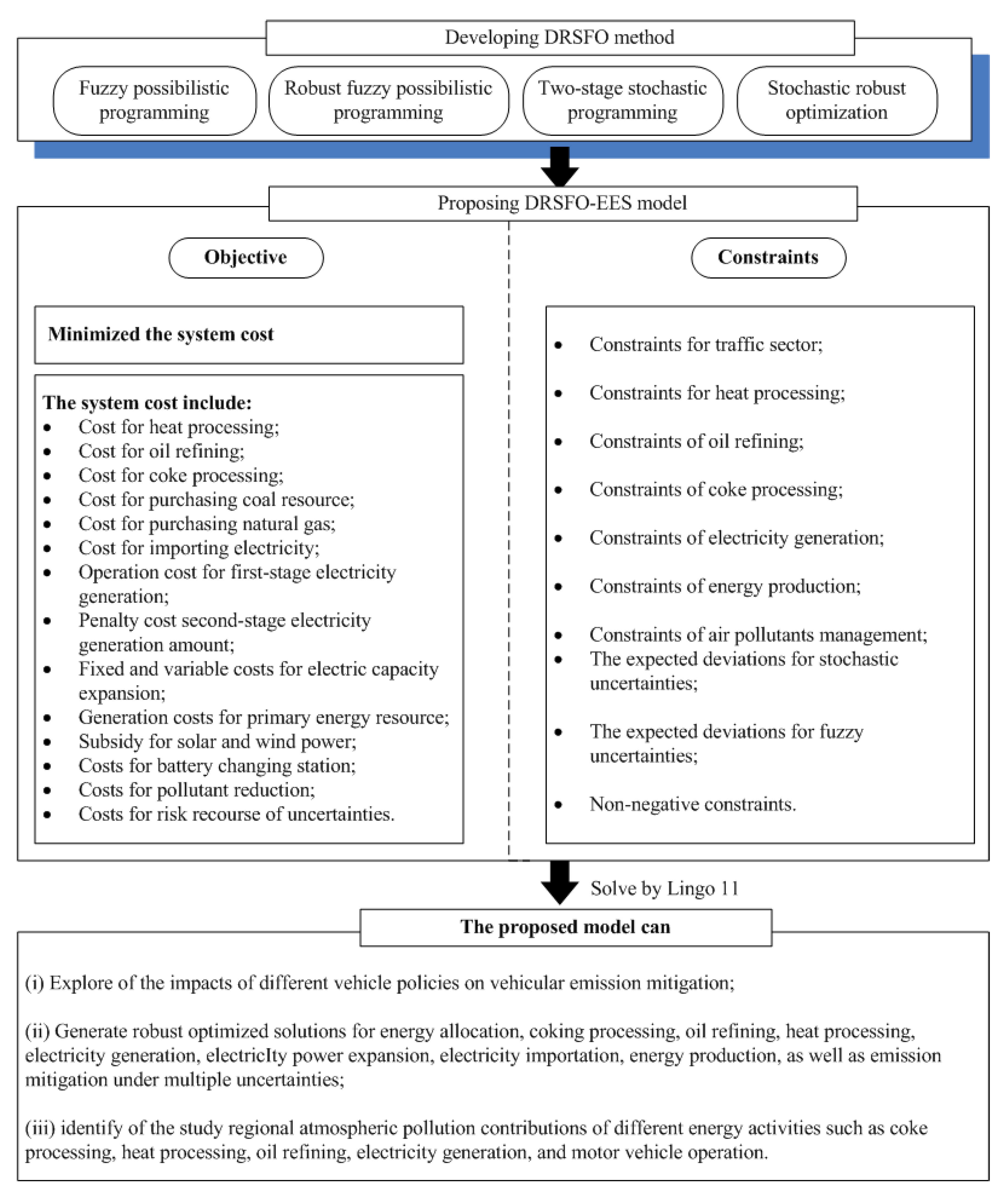
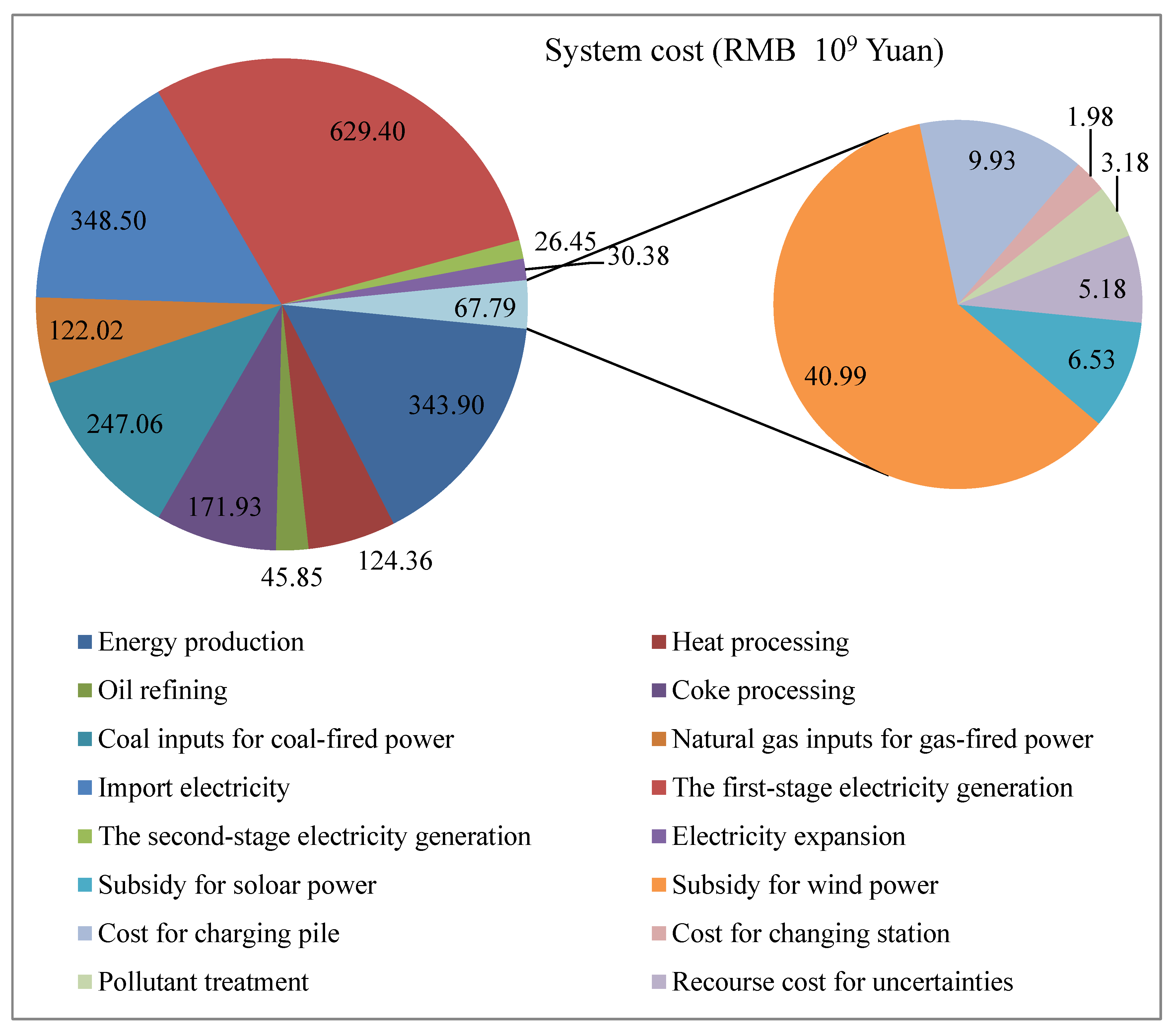
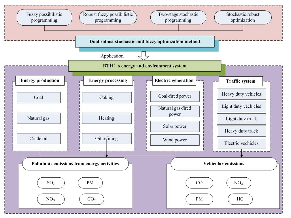
Minimizing the system cost is the objective of DRSFO-EES, which includes costs for coke processing, heat processing, input for coal-based power, oil refining, input for natural gas-based power, imported electricity, first-stage of electricity generation, second-stage of electricity generation, electricity expansion, energy production, subsidy for solar power generation, subsidy for wind power generation, EVs charging piles, EVs charging stations, pollutants treatment, and risk recourse for the stochastic and fuzzy uncertainties. The proposed DRSFO-EES can be solved by Lingo 11.0 software. The schematic diagram of DRAOM-EWNS model is presented in Figure 2.
In the DRSFO-EES, t denotes the planning periods, period 1 (2020), period 2 (2025), and period 3 (2030); i denotes the primary energy production type, i = 1 is coal, i = 2 is natural gas, and i = 3 is crude oil; k denotes the electric conversion technology, k = 1 is coal-based power, k = 2 is natural gas-based power, k = 3 is solar power, and k = 4 is wind power; h expresses the electricity demand-level, h = 1 (low demand level), h = 2 (medium demand level), h = 3 (high demand level), h = 1 3 p h = 1 ; g are the vehicles types, g = 1 is HDVs, g = 2 is LDVs, g = 3 is TDTs, g = 4 is HDTs, and g = 5 is others. The proposed DRSFO-EES is formulated as follows:
Objective:
Min   f ˜ = f ¯ + λ 1 ( f max f ¯ ) + λ 2 ( f ¯ f min ) + V F t = f 1   +   f 2   +   f 3   +   f 4 +   f 5   +   f 6   +   f 7 +   f 8 +   f 9   +   f 10     f 11 f 12 + f 13   +   f 14   +   f 15 +   f 16  
where f ˜ represents the system cost; f ˜ 1 denotes the heat processing cost; f ˜ 2 denotes oil refining cost; f ˜ 3 denotes coke processing cost; f ˜ 4 denotes the cost of coal inputs for coal-based power; f ˜ 5 denotes the cost of natural gas inputs for natural gas-based power; f ˜ 6 denotes importing electricity cost; f ˜ 7 denotes the cost of first-stage electricity generation; f ˜ 8 denotes the cost of second-stage electricity generation; f ˜ 9 denotes electricity expansion cost; f ˜ 10 denotes the energy production cost; f ˜ 11 denotes the subsidy for solar power; f ˜ 12 denotes the subsidy for wind power; f ˜ 13 denotes the cost of charging pile; f ˜ 14 denotes the cost of changing station; f ˜ 15 denotes air-pollutants removal cost; f ˜ 16 denotes the risk recourse costs of stochastic and fuzzy uncertainties. V F t represents the positive deviation between maximum values and worst value of fuzzy parameters. λ 1 and λ 2 represent their respective weight coefficients, where it is assumed λ 1 and λ 2 are fixed (i.e., λ 1 = λ 2 = 1).
(1) Cost of heat processing. This cost is used for heat processing, and it is calculated based on the unit-price and amount of heat processing.
f ˜ 1 = t = 1 3 [ 0.25 · ( H P P t 1 + 2 H P P t 2 + H P P t 3 )   · H G A t +   λ 1 · t = 1 3 [ H P P t 3 0.25 · ( H P P t 1 + 2 · H P P t 2 + H P P t 3 ) ] ·   H G A t +   λ 2 · t = 1 3 [ 0.25 · ( H P P t 1 + 2 · H P P t 2 + H P P t 3 ) H P P t 1 ] ·   H G A t
where H P ˜ P t ( H P P i t 1 , H P P i t 2 , H P P i t 3 ) is the cost for unit of heat processing, which is expressed as a triangular fuzzy number; H G A t is the heat processing amount.
(2) Cost for oil refining. This cost is calculated in terms of the unit-price and the amount of oil refining.
f ˜ 2 = t = 1 3 [ 0.25 · ( P V O t 1 + 2 · P V O t 2 + P V O t 3 )   · O F O I L t +   λ 1 · t = 1 3 [ P V O t 3 0.25 · ( P V O t 1 + 2 · P V O t 2 + P V O t 3 ) ] · O F O I L t +   λ 2 · t = 1 3 [ 0.25 · ( P V O t 1 + 2 · P V O t 2 + P V O t 3 )   P V O t 1 ] ·   O F O I L t
where P V ˜ O t   ( P V O t 1 , P V O t 2 , P V O t 3 ) is the cost for unit of oil refining; O F O I L t is the crude oil consumption of oil refining. (3) Cost for coke processing. This cost is calculated in terms of the unit-price and the amount of coke processing.
f ˜ 3 = t = 1 3 [ 0.25 · ( P W O t 1 + 2 · P W O t 2 + P W O t 3 )   · C K P A t +   t = 1 3 [ P W O t 3 0.25 · ( P W O t 1 + 2 · P W O t 2 + P W O t 3 ) ]   · C K P A t +   t = 1 3 [ 0.25 · ( P W O t 1 + 2 · P W O t 2 + P W O t 3 )   P W O t 1 ] ·   C K P A t
where P W ˜ O t ( P W O t 1 , P W O t 2 , P W O t 3 ) is the cost for unit of coke processing; and C K P A t is the coke processing amount.
(4) Cost for purchasing coal resources. This cost is used for purchasing coal resources, and it is calculated based on the unit-price and the amount of coal resource.
f ˜ 4 = t = 1 3 [ 0.25 · ( N S C t 1 + 2 · N S C t 2 + N S C t 3 ) ]   · E C O A L M t +   λ 1 · t = 1 3 [ N S C t 3 0.25 · ( N S C t 1 + 2 · N S C t 2 + N S C t 3 ) ] · E C O A L M t +   λ 2 · t = 1 3 [ 0.25 · ( N S C t 1 + 2 · N S C t 2 + N S C t 3 )   N S C t 1 ] ·   E C O A L M t
where N S ˜ C t ( N S C t 1 , N S C t 2 , N S C t 3 ) is the price for unit of coal resource; and E C O A L M t is the coal consumption of coal-based power.
(5) Cost for purchasing natural gas resources. This cost is used for purchasing natural gas resources, and it is calculated based on the unit-price and the amount of natural gas resource.
f ˜ 5 = t = 1 3 [ 0.25 · ( N S N t 1 + 2 · N S N t 2 + N S N t 3 ) ]   · E N G M t +   λ 1 · t = 1 3 [ N S N t 3 0.25 · ( N S N t 1 + 2 · N S N t 2 + N S N t 3 ) ] · E N G M t +   λ 2 · t = 1 3 [ 0.25 · ( N S N t 1 + 2 · N S N t 2 + N S N t 3 )   N S N t 1 ] ·   E N G M t
where N S ˜ N t ( N S N t 1 ,   N S N t 2 ,   N S N t 3 ) is the price for unit of natural gas resource; and E N G M t is the natural gas consumption of natural gas-based power.
(6) Cost for importing electricity. This cost is calculated in terms of the unit-price and the amount of importing electricity.
f ˜ 6 = t = 1 3 h = 1 3 [ 0.25 · ( N E t 1 + 2 · N E t 2 + N E t 3 )   · E D t h +   λ 1 · t = 1 3 h = 1 3 [ N E t 3 0.25 · ( N E t 1 + 2 · N E t 2 + N E t 3 ) ] · E D t h +   λ 2 · t = 1 3 h = 1 3 [ 0.25 · ( N E t 1 + 2 · N E t 2 + N E t 3 )   N E t 1 ] ·   E D t h
where N E ˜ t ( N E t 1 ,   N E t 2 ,   N E t 3 ) is the price for unit of imported electricity; E D t h is the amount of imported electricity.
(7) Operation cost for first-stage electricity generation. The cost represents the operation cost of first-stage electricity generation facilities (i.e., coal-based power, gas-based power, wind power and solar power) during the planning periods. It is calculated in terms of the operation costs and the amount of electricity generation for each of the electricity generation facilities. Furthermore, the first-stage is given by W k t ± = W k t + r r k t · Δ W , where r r k t denotes the decision variables, Δ W = W k t + W k t .
f ˜ 7 = k = 1 4 t = 1 3 [ 0.25 · ( P V k t 1   +   2 · P V k t 2 + P V k t 3 )   ] ·   ( W k t + r r k t · Δ W k t ) + λ 1 k = 1 4 t = 1 3 [ P V i t 3 0.25 · ( P V k t 1   +   2 · P V k t 2 + P V k t 3 )   ] ·   ( W k t + r r k t · Δ W k t ) + λ 2 k = 1 4 t = 1 3 [ 0.25 · ( P V k t 1   +   2 · P V k t 2 + P V k t 3 )   P V k t 1 ] ·   ( W k t + r r k t · Δ W k t )
where P V ˜ k t ( P V k t 1 ,   P V k t 2 ,   P V k t 3 ) denotes the operation cost of different power conversion technologies; W k t ± = W k t + r r k t · Δ W k t is the first-stage electricity generation amount, which is determined by decision variables r r k t ( Δ W = W k t + W k t and r r k t [ 0 ,   1 ] ).
(8) Penalty cost for second-stage electricity generation amounts (i.e., shortage electricity amount of first-stage). It is calculated in terms of the penalty costs and the amount of second-stage electricity generation by each electricity generation technology.
f ˜ 8 = k = 1 4 t = 1 3 h = 1 3 [ 0.25 · ( P P k t 1 + 2 · P P k t 2 +   P P k t 3 ) ] · p t h · Y k t h +   λ 1 · k = 1 4 t = 1 3 h = 1 3 [ P P k t 3 0.25 · ( P P k t 1 + 2 · P P k t 2 +   P P k t 3 ) ] ·   p t h · Y k t h + λ 2 · k = 1 4 t = 1 3 h = 1 3 [ 0.25 · ( P P k t 1 + 2 · P P k t 2 +   P P k t 3 ) P P k t 1 ] ·   p t h · Y k t h
where P P ˜ k t ( P P k t 1 ,   P P k t 2 ,   P P k t 3 ) is the operating cost for the second-stage electricity generation amount ( Y k t h ). Y k t h is the second-stage electricity generation amount.
(9) Fixed and variable costs for electric capacity expansion. These costs include the fixed and variable electric capacity expansion costs of four electricity generation technologies in the planning horizon.
f ˜ 9 = i = 1 4 t = 1 3 h = 1 3 p t h · [ 0.25 · ( A k t 1 + 2 · A k t 2 +   A k t 3 ) ] · Q k t h + λ 1 · i = 1 4 t = 1 3 h = 1 3 p t h · [ A k t 3 0.25 · ( A k t 1 + 2 · A k t 2 +   A k t 3 ) ] · Q k t h + λ 2 · i = 1 4 t = 1 3 h = 1 3 p t h · [ 0.25 · ( A k t 1 + 2 · A k t 2 +   A k t 3 ) A k t 1 ] · Q k t h + i = 1 4 t = 1 3 h = 1 3 p t h · [ 0.25 · ( B k t 1 + 2 · B k t 2 +   B k t 3 ) ] · Z k t h + λ 1 · i = 1 4 t = 1 3 h = 1 3 p t h · [ B k t 3 0.25 · ( B k t 1 + 2 · B k t 2 +   B k t 3 ) ] · Z k t h + λ 2 · i = 1 4 t = 1 3 h = 1 3 p t h · [ 0.25 · ( B k t 1 + 2 · B k t 2 +   B k t 3 ) B k t 1 ] · Z k t h
where A ˜ k t ( A k t 1 , A k t 2 , A k t 3 ) denote fixed-charge cost for different electric capacity expansion. Q k t h are binary variables for identifying whether or not the capacity expansion needs to be undertaken by power conversion technology k. B ˜ k t ( B k t 1 , B k t 2 , B k t 3 ) denote the variable cost of capacity expansion. Z k t h denotes the continuous variable of the capacity expansion amount.
(10) Generation costs for primary energy resources. This cost is calculated in terms of the unit-price of primary energy (i.e., coal, natural gas, and crude oil) and the amount of primary generation.
f ˜ 10 = i = 1 3 t = 1 3 0.25 · ( E P P i t 1   + 2 · E P P i t 2 + E P P i t 3 ) ·   E P A i t + λ 1 · i = 1 3 t = 1 3 [ E P P i t 3 0.25 · ( E P P i t 1 + 2 · E P P i t 2 + E P P i t 3 ) ] ·   E P A i t + λ 2 · i = 1 3 t = 1 3 [ 0.25 · ( E P P i t 1 + 2 · E P P i t 2 + E P P i t 3 ) E P P i t 1 ] ·   E P A i t
where E P ˜ P i t ( E P P i t 1 , E P P i t 2 , E P P i t 3 ) is the production cost per unit of energy resource; and E P A i t is the production amount.
(11) Subsidy for solar power. The government provides a subsidy for units of electricity generated by solar power, and it is calculated in terms of the unit-subsidy of solar power and the amount of electricity generation amount of solar power.
f ˜ 11 = t = 1 3 [ 0.25 · ( S P t 1 + 2 · S P t 2 + S P t 3 )   · ( W 3 t + r r 3 t · Δ W 3 t ) +   t = 1 3 [ S P t 3 0.25 · ( S P t 1 + 2 · S P t 2 + S P t 3 ) ]   · ( W 3 t + r r 3 t · Δ W 3 t ) +   t = 1 3 [ 0.25 · ( S P t 1 + 2 · S P t 2 + S P t 3 )   S P t 1 ] ·   ( W 3 t + r r 3 t · Δ W 3 t )
where S P ˜ t ( S P t 1 , S P t 2 , S P t 3 ) is the solar subsidy provided by government for unit of electricity generated by solar power.
(12) Subsidy for wind power. The government provides a subsidy for units of electricity generated by wind power, and it is calculated in terms of the unit-subsidy of wind power and the amount of electricity generation amount of wind power.
f ˜ 12 = t = 1 3 [ 0.25 · ( W P t 1 + 2 · W P t 2 + W P t 3 )   · ( W 4 t + r r 4 t · Δ W 4 t ) +   t = 1 3 [ W P t 3 0.25 · ( W P t 1 + 2 · W P t 2 + W P t 3 ) ]   · ( W 4 t + r r 4 t · Δ W 4 t ) +   t = 1 3 [ 0.25 · ( W P t 1 + 2 · W P t 2 + W P t 3 )   W P t 1 ] ·   ( W 4 t + r r 4 t · Δ W 4 t )
where W P ˜ t ( W P t 1 , W P t 2 , W P t 3 ) is the wind subsidy provided by government for unit of electricity generated by wind power.
(13) Costs for battery charging piles. It is calculated in terms of the average charging pile amount for unit of electric vehicle, the EVs population, as well as the investment cost per EV charging pile.
f 13 = t = 1 3 E V A t · R E C t · F C D t
where E V A t is the EVs population; R E C t is the average charging pile amount for unit of electric vehicle; F C D t is the investment cost per EV charging pile.
(14) Costs for battery changing station. It is calculated in terms of the average changing station amount for unit of electric vehicle, the EVs population, as well as the investment cost per EV changing station.
f 14 = t = 1 3 E V A t · R E V t · F V D t
where R E V t is the average changing station amount for unit of electric vehicles; F V D t is the investment cost per EV changing station.
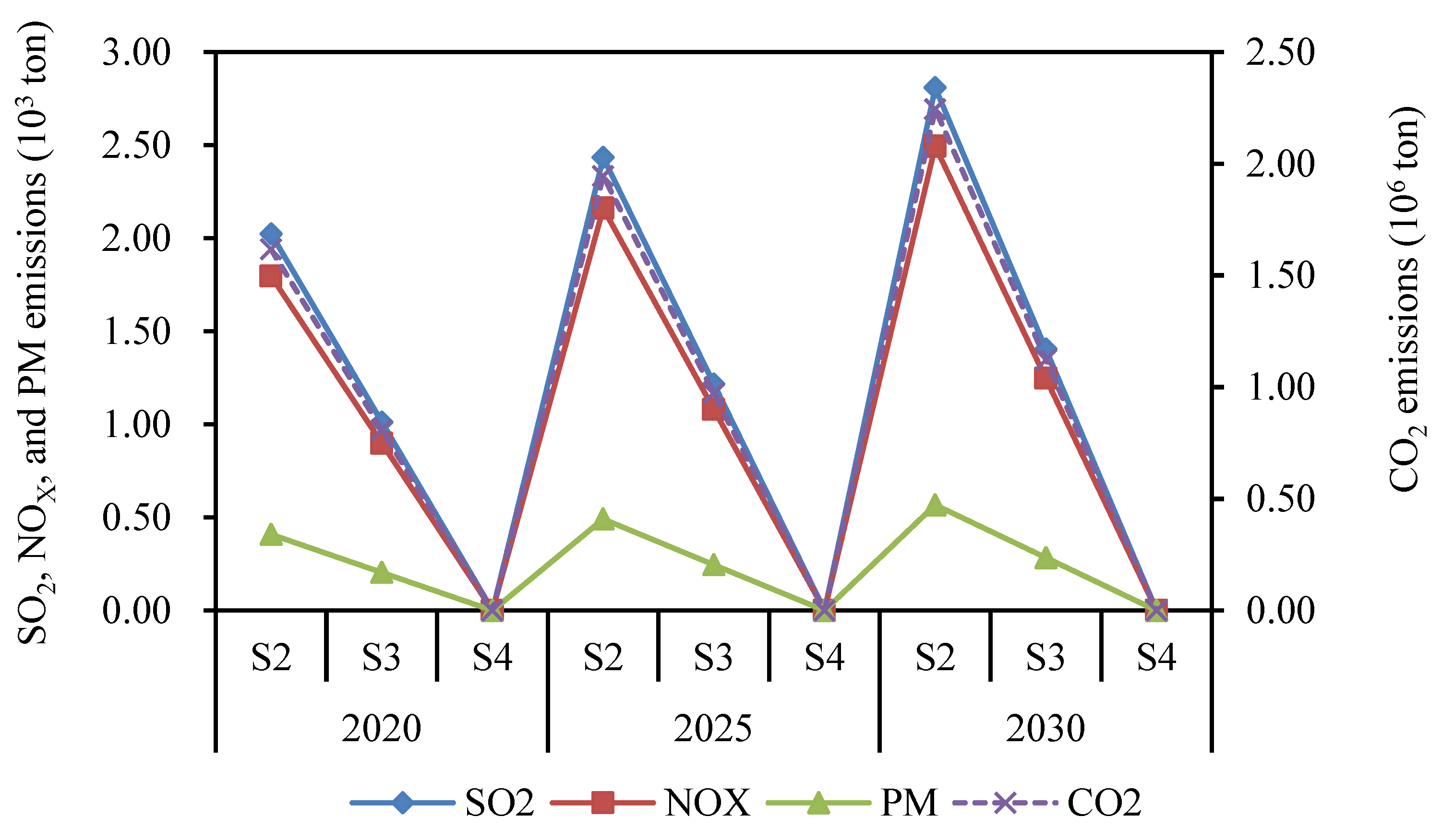
(15) Costs for pollutant reduction. These costs include reduction costs for three pollutants, i.e., SO2, NOX, and PM emissions.
f ˜ 15 =   f ˜ 15 s + f ˜ 15 N + f ˜ 15 P M
where   f ˜ 15 s is the cost of desulfurization; S O 2 K t is the SO2 emissions from coking processing; S O 2 C E t is the SO2 emissions from coal-based power; S O 2 N E t is the SO2 emissions from natural gas-based power; S O 2 H t is the SO2 emissions from heating processing; S O 2 O t is the SO2 emissions from oil refining; T P ˜ S t ( T P S t 1 , T P S t 2 , T P S t 3 ) is the desulfurization cost of per unit of SO2 emission; η s is the desulfurization efficiency.
(15a) Costs for SO2 emissions reduction. The cost is calculated in terms of the total SO2 emissions, the desulfurization cost per unit of SO2 emission, and the desulfurization efficiency.
f ˜ 15 S =   { t = 1 3 ( S O 2 K t + S O 2 C E t +   S O 2 N E t + S O 2 H t +   S O 2 O t )   · 0.25 ·   ( T P S t 1 + T P S t 2 + T P S t 3   ) ·   η s } + λ 1 · { t = 1 3 ( S O 2 K t + S O 2 C E t +   S O 2 N E t + S O 2 H t +   S O 2 O t ) · [ T P S t 3   0.25 ·   ( T P S t 1 + T P S t 2 + T P S t 3   ) ] ·   η s } + λ 2 · { t = 1 3 ( S O 2 K t + S O 2 C E t +   S O 2 N E t + S O 2 H t +   S O 2 O t ) · [ 0.25 ·   ( T P S t 1 + T P S t 2 + T P S t 3   ) T P S t 1 ] ·   η s }
where   f ˜ 15 s is the cost of desulfurization; S O 2 K t is the SO2 emissions from coking processing; S O 2 C E t is the SO2 emissions from coal-based power; S O 2 N E t is the SO2 emissions from natural gas-based power; S O 2 H t is the SO2 emissions from heating processing; S O 2 O t is the SO2 emissions from oil refining; T P ˜ S t ( T P S t 1 , T P S t 2 , T P S t 3 ) is the desulfurization cost per unit of SO2 emission; η s is the desulfurization efficiency.
(15b) Costs for NOX emissions reduction. The cost is calculated in terms of the total NOx emissions, the desulfurization cost per unit of NOx emission, and the desulfurization efficiency.
f ˜ 15 N =   { t = 1 3 ( N O X K t + N O X C E t +   N O X N E t + N O X H t +   N O X O t )   · 0.25 ·   ( T P N t 1 + T P N t 2 + T P N t 3   ) ·   η N } + λ 1 · { t = 1 3 ( N O X K t + N O X C E t +   N O X N E t + N O X H t +   N O X O t ) · [ T P N t 3   0.25 ·   ( T P N t 1 + T P N t 2 + T P N t 3   ) ] ·   η N } + λ 2 · { t = 1 3 ( N O X K t + N O X C E t + N O X N E t + N O X H t + N O X O t ) · [ 0.25 ·   ( T P N t 1 + T P N t 2 + T P N t 3   ) T P N t 1 ] ·   η N }
where f ˜ 15 N is the cost of denitration; N O X K t is the NOx emissions from coking processing; N O X C E t is the NOx emissions from coal-based power; N O X N E t is the NOx emissions from natural gas-based power; N O X H t is the NOx emissions from heat processing; N O X O t is the NOx emissions from oil refining; T P ˜ N t ( T P N t 1 , T P N t 2 , T P N t 3 ) is the denitration cost per unit of NOx emission; η N is the denitration efficiency.
(15c) Costs for PM emissions reduction. The cost is calculated in terms of the total PM emissions, the desulfurization cost per unit of PM emission, and the desulfurization efficiency.
f ˜ 15 P M =   { t = 1 3 ( P M K t + P M C E t +   P M N E t + P M H t +   P M O t )   · 0.25 ·   ( T P P M t 1 + T P P M t 2 + T P P M t 3   ) ·   η P M } + λ 1 · { t = 1 3 ( P M K t + P M C E t +   P M N E t + P M H t + P M O t ) · [ T P P M t 3   0.25 ·   ( T P P M t 1 + T P P M t 2 + T P P M t 3   ) ] ·   η P M } + λ 2 · { t = 1 3 ( P M K t + P M C E t + P M N E t + P M H t + P M O t ) · [ 0.25 ·   ( T P P M t 1 + T P P M t 2 + T P P M t 3   ) T P P M t 1 ] ·   η P M }
where   f ˜ 15 P M is the PM removal cost; P M K t is the PM emissions from coking processing; P M C E t is the PM emissions from coal-based power; P M N E t is the PM emissions from natural gas-based power; P M H t is the PM emissions from heating processing; P M O t is the NOX emissions from oil refining; T P ˜ P M t ( T P P M t 1 , T P P M t 2 , T P P M t 3 ) is the treatment cost per unit of PM emission; η P M is the PM removal efficiency.
(16) Costs for risk recourse of stochastic and fuzzy uncertainties.
f ˜ 16 = V T ˜ S + V T ˜ F = ρ 1 · i = 1 I t = 1 T h = 1 H p t h ( V i t h + V C i t h ] + ρ 2 · t = 1 3 V F t
where V T ˜ S denotes the risk recourse cost for stochastic uncertainties; V T ˜ F denotes the risk recourse cost of fuzzy uncertainties, with capturing the difference between the extreme values of fuzzy parameters. The nonnegative factors ρ1 and ρ2 represent robust levels (its range from 0 to 1), which can help managers make trade-offs between system economy and reliability.
Constraints:
The constraints of the proposed DRSFO-EES model include traffic sector, heat processing, coke processing, oil refining, electricity generation, energy production, air-pollutants treatment, and risk recourse cost for stochastic uncertainties and risk recourse for fuzzy uncertainties.
(1) Constraints for traffic sector.
This constraint represents that the optimized vehicles population must be not less than the lower bounds of vehicle population. C r { M A ˜ L g t | M A g t M A ˜ L g t } α means the credibility of the M A g t M A ˜ L g t is higher than or equal to confidence-level α.
C r { M A ˜ L g t | M A g t M A ˜ L g t } α
where M A g t is the optimized solutions of vehicles population; M A ˜ L g t ( M A L g t 1 ,   M A L g t 2 ,   M A L g t 3 ) is the lower bounds of vehicle population, which is expressed as a triangular fuzzy number.
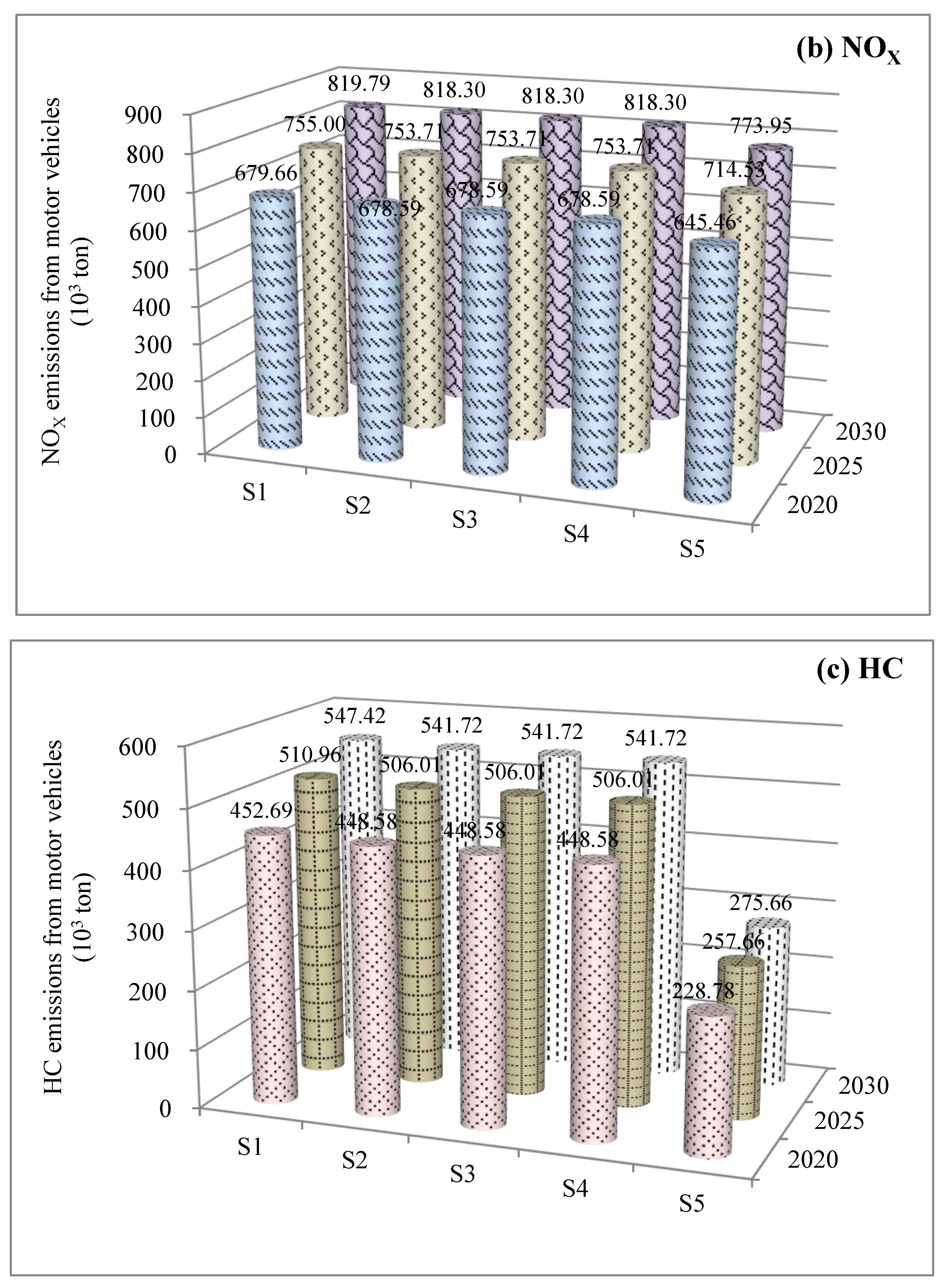
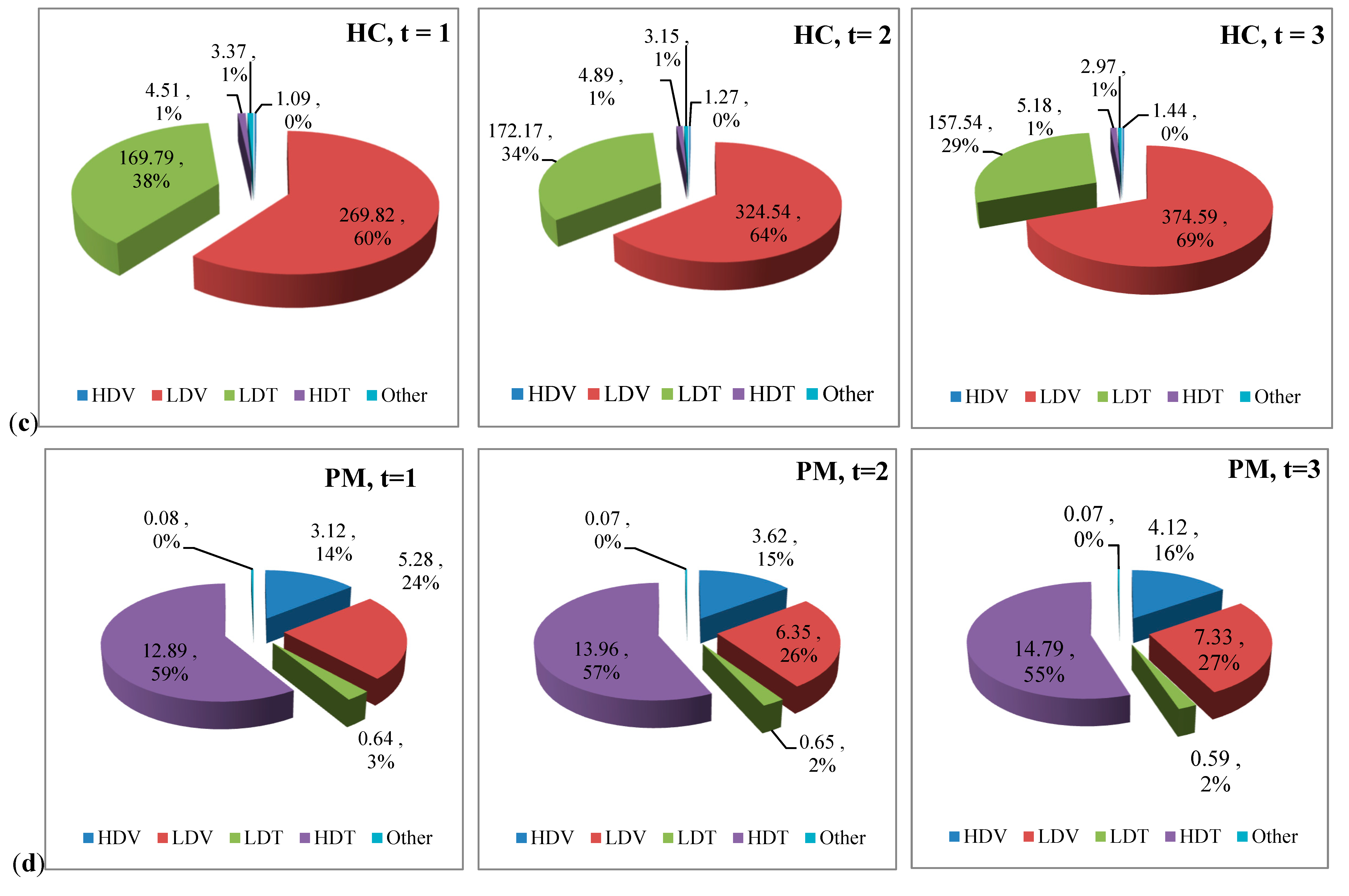
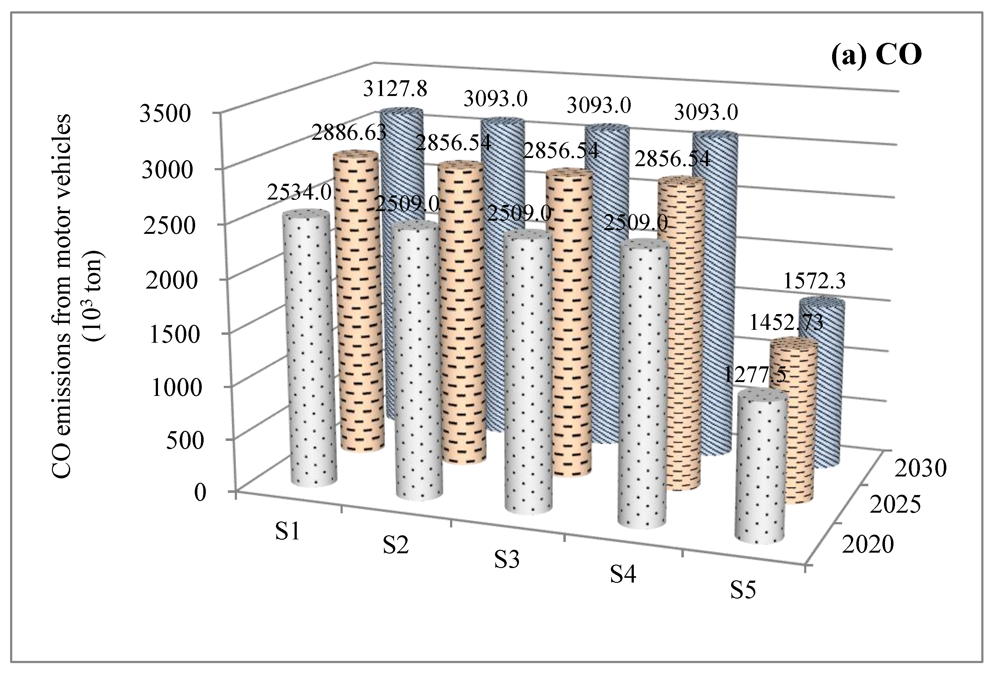
Constraints for vehicle-emissions, including CO, NOx, HC, and PM emissions. These constraints represent that the vehicle-emissions are calculated in terms of the annual average mileage, the proportion of electric vehicles and the emission factors of CO, NOx, HC and PM emissions.
T R C O g t | g = 1 , 3 , 4 , 5 = M A g t | g = 1 , 3 , 4 , 5 · M Q g t | g = 1 , 3 , 4 , 5 · T R C O E g t | g = 1 , 3 , 4 , 5
T R C O 2 t = ( M A g t M A g t · R E V t ) · M Q g t · T R C O E g t
T R N O X g t | g = 1 , 3 , 4 , 5 = M A g t | g = 1 , 3 , 4 , 5 · M Q g t | g = 1 , 3 , 4 , 5 · T R N O E g t | g = 1 , 3 , 4 , 5
T R N O X 2 t = ( M A g t M A g t · R E V t ) · M Q g t · T R N O E g t
T R H C g t | g = 1 , 3 , 4 , 5 = M A g t | g = 1 , 3 , 4 , 5 · M Q g t | g = 1 , 3 , 4 , 5 · T R H C g t | g = 1 , 3 , 4 , 5
T R H C 2 t = ( M A g t M A g t · R E V t ) · M Q g t · T R H C g t
T R P M g t | g = 1 , 3 , 4 , 5 = M A g t | g = 1 , 3 , 4 , 5 · M Q g t | g = 1 , 3 , 4 , 5 · T R P M g t | g = 1 , 3 , 4 , 5
T R P M 2 t = ( M A g t M A g t · R E V t ) · M Q g t · T R P M g t
where T R C O g t is CO emissions from vehicle g in period t; M Q g t is the annual average mileage; R E V t is the proportion of electric vehicles; T R C O E g t the emission factor of CO; T R N O E g t the emission factor of NOX; T R H C g t the emission factor of HC; T R P M g t the emission factor of PM.
Constraints of the electricity demands of EVs. This constraint is calculated in terms of the electricity consumption amounts per hundred kilometers of EVs and the amount of EVs.
E V E C t = M A 2 t · R E V t · M Q 2 t · E C P E V t
where E V E C t is the electricity consumption amounts of EVs; E C P E V t is the electricity consumption amounts per hundred kilometers of EVs.
(2) Constraints of heat processing. Constraint (52) depicts that the heat generation amounts must not be less than the heat demands, and C r { D M ˜ H t | H G A t D M ˜ H t } α means the credibility of the H G A t D M ˜ H t is higher than or equal to confidence-level α. Constraints (53) and (54) represent the consumption amounts of natural gas and coal for heat processing.
C r { D M ˜ H t | H G A t D M ˜ H t } α
C F H G C t = C F H t · H G A t · H C P t
C F H G N t = C F H t · H G A t · H N P t
where D M ˜ H t ( D M H t 1 , D M H t 2 , D M H t 3 ) is the heat demand; C F H t denotes the energy consumption for the unit of kerosene processing. C F H G C t denotes the coal consumption of heat processing; C F H G N t is the natural gas consumption of heat processing; H C P t denotes the ratio of coal consumption of heat processing; H N P t denotes the ratio of natural gas consumption of heat processing.
(3) Constraints of oil refining. The constraint depicts the input amounts of crude oil for oil refining.
O F O I L t = Z C Y t · Z C Y E t + Z Q Y t · Z Q Y E t + Z M Y t · Z M Y E t +   Z R L Y t   ·   Z R L Y E t   +   Z S N Y t   ·   Z S N Y E t +   Z S J Y t   ·   Z S J Y E t   +   Z L P G t   ·   Z L P G E t   +   Z Q T t
where Z C Y t is the diesel processing amount; Z C Y E t denotes the crude oil consumption for unit of diesel processing; Z Q Y t is the processing amount of gasoline; Z Q Y E t denote the crude oil consumption for unit of gasoline processing; Z M Y t is the processing amount of kerosene; Z M Y E t denotes the crude oil consumption for unit of kerosene processing; Z R L Y t is the fuel oil processing amount; Z R L Y E t is the crude consumption for unit of fuel oil processing; Z S N Y t is the processing amount for naphtha; Z S N Y E t denotes the crude oil consumption for unit of naphtha processing; Z S J Y t is the processing amount of asphaltic pyrobitumen; Z S J Y E t denotes the crude oil consumption for unit of asphaltic pyrobitumen processing; Z L P G t is the processing amount of LPG; Z L P G E t denotes the crude consumption for unit of LPG processing; Z Q T t denotes the crude oil consumption of other oil products.
(4) Constraints of coke processing. Constraint (56) means that the amount of coke processing is not less than the coke demands, and C r { D M C ˜ J t | C K P A t D M C ˜ J t } α means the credibility of the C K P A t D M C ˜ J t is higher than or equal to confidence-level α. Constraint (57) depicts the coal consumption amount for coke processing.
C r { D M C ˜ J t | C K P A t D M C ˜ J t } α
C F C J t   =   C K P A t / C T C K E t
where D M C ˜ J t ( D M C J t 1 , D M C J t 2 , D M C J t 3 ) is the coke demand expressed as a triangular fuzzy number. C T C K E t denotes the coal consumption for unit of coke processing; C F C J t is the coal consumption of coke processing.
(5) Constraints of electricity generation.
Constraints for mass balance of coal and natural gas resources. These constraints are established to calculate the consumption amounts of coal and natural gas for electricity generation.
[ ( W 1 t + r r 1 t · W C 1 t ) + Y 1 t h + E V E C t ] · F E 1 t = E C O A L M t
[ ( W 2 t + r r 2 t · W C 2 t ) + Y 2 t h ] · F E 2 t = E N G M t
where F E i t is the coal (i = 1) and natural gas (i = 2) consumption for a unit of electricity generation.
Constraints of electricity demand and supply balance. Constraint (60) is established to ensure the electricity demand be satisfied by domestic electricity generation and importation. And C r { D ˜ t h | i = 1 4 t = 1 3 [ ( W i t + r r i t · W C i t ) + Y i t h + E V E C t ] + E d t h D ˜ t h } α means the credibility of the i = 1 4 t = 1 3 [ ( W i t + r r i t · W C i t ) + Y i t h + E V E C t ] + E d t h D ˜ t h is higher than or equal to confidence-level α. For constraint (61), the optimized amount of electricity generated in the first-stage is given by W k t ± = W k t + r r k t · Δ W , where r r k t denotes the decision variables, and r r k t [ 0 ,   1 ] .
C r { D ˜ t h | i = 1 4 t = 1 3 [ ( W i t + r r i t · W C i t ) + Y i t h + E V E C t ] + E d t h D ˜ t h } α
0 r r i t 1
where D ˜ t h is the electricity demand under various electricity demand levels, which show the characteristics of stochastic and fuzzy sets. r r i t denotes the decision variable of first-stage electricity generation.
Constraints for electricity capacities. These constraints mainly depict that the amount of generated electricity must not exceed its existing and expanded capacities, which are established to ensure that the available electricity-generation capacity is greater than the generated electricity.
i = 1 4 ( W i t + r r i t · W C i t ) + Y i t h + E V E C t i = 1 2 [ C F i t · ( R C i t + Z i t h ) ]
i = 1 4 ( R C i + Z i t h ) U t ; t ,   h
i = 1 4 ( R C i + Z i t h ) U S t ; t ,   h
i = 1 4 Y i t h i = 1 4 C F i t · Z i t h
0 Y i t h ( W i t + r r i t · W C i t ) ; i ,   t ,   h
Q i t h = { = 1 ,   if   capacity   expansion   of   is   undertaken   i ,   t ,   h = 0 ,   if   otherwise
where C F k t is the operating hours of electricity conversion technology k; R C k t is the original capacity; U t is the lower bound of load demands; U S t is the upper bound of load demands.
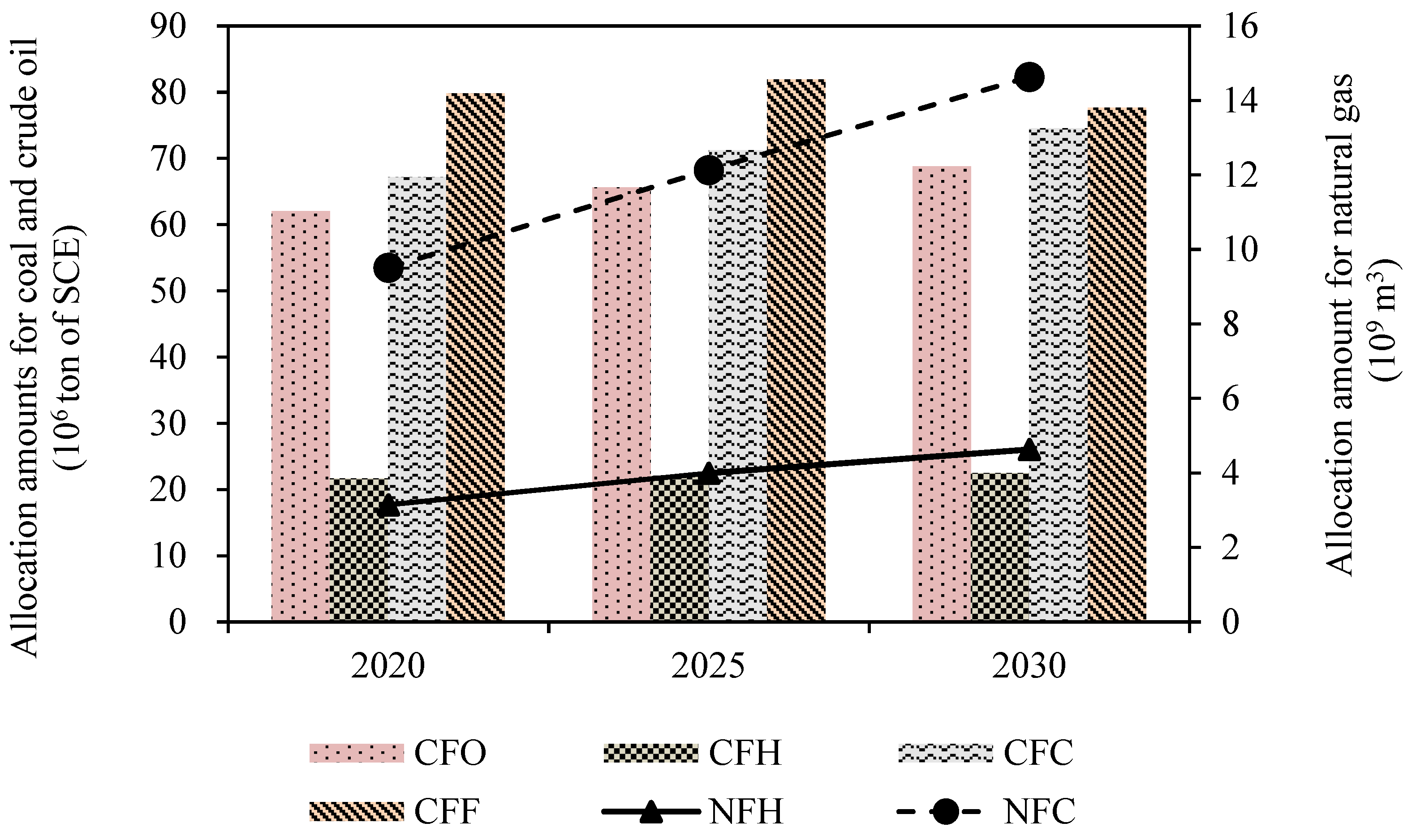
(6) Constraints of energy production. The constraint is established to ensure the primary energy production amount must be less than the lower bound and higher than the upper bound.
E P A L E P A i t     E P A U i t
where E P A U i t is the upper bound of amount of primary energy production. E P A L i t is the lower bound of amount of primary energy production.
(7) Constraints for air-pollutants management.
SO2 emissions. Constraints (69) to (74) represent the SO2 emissions from energy activities (i.e., coke processing, heat processing, electricity generation, and oil refining). Constraints (74) are used for ensuring that the SO2-emissions are satisfied by the pollutant-emission permits.
S O 2 K t = C F C J t · C S t
S O 2 C E t = E C O A L M t ·   C S t
S O 2 N E t = N E G M t · C S t
S O 2 H t = C F H G C t · C S t + C F H G N t · N S t
S O 2 O t = O F O I L t · O S t
( S O 2 K t + S O 2 C E t + S O 2 N E t + S O 2 H t + S O 2 O t )   ·   ( 1 η s )     T S t
where C S t is the SO2 emission factor of coal; N S t is the SO2 emission factor of natural gas; O S t is the SO2 emission factor of crude oil; η s is the desulfurization efficiency; T S t is the upper bounds of SO2 emission.
NOX emissions. Constraints (75) to (79) represent the NOx emissions from energy activities (i.e., coke processing, heat processing, electricity generation, and oil refining). Constraints (80) are used for ensuring that the NOx-emissions are satisfied by the pollutant-emission permits.
N O X K t = C F C J t · C N t
N O X C E t = E C O A L M t ·   C N t
N O X N E t = N E G M t · N N t
N O X H t = C F H G C t · C N t + C F H G N t · N N t
N O X O t = O F O I L t · O N t
( N O X K t + N O X C E t + N O X N E t + N O X H t + N O X O t )   ·   ( 1 η N )     T N t
where C N t is the NOx emission factor of coal; N N t is the NOx emission factor of natural gas; O N t is the NOx emission factor of crude oil; η N is the denitration efficiency; T N t is the upper bounds of NOx emission.
PM emissions. Constraints (81) to (85) represent the PM emissions from energy activities (i.e., coke processing, heat processing, electricity generation, and oil refining). Constraints (86) are used for ensuring that the PM-emissions are satisfied by the pollutant-emission permits.
P M K t = C F C J t · C P M t
P M C E t = E C O A L M t ·   C P M t
P M N E t = N E G M t · N P M t
P M H t = C F H G C t · C P M t + C F H G N t · N P M t
P M O t = O F O I L t · O P M t
( P M K t + P M C E t + P M N E t + P M H t + P M O t )   ·   ( 1 η P M )     T P M t
where C P M t is the PM emission factor of coal; N P M t is the PM emission factor of natural gas; O P M t is the PM emission factor of crude oil; η P M is the PM removal efficiency; T P M t is the upper bound of PM emission.
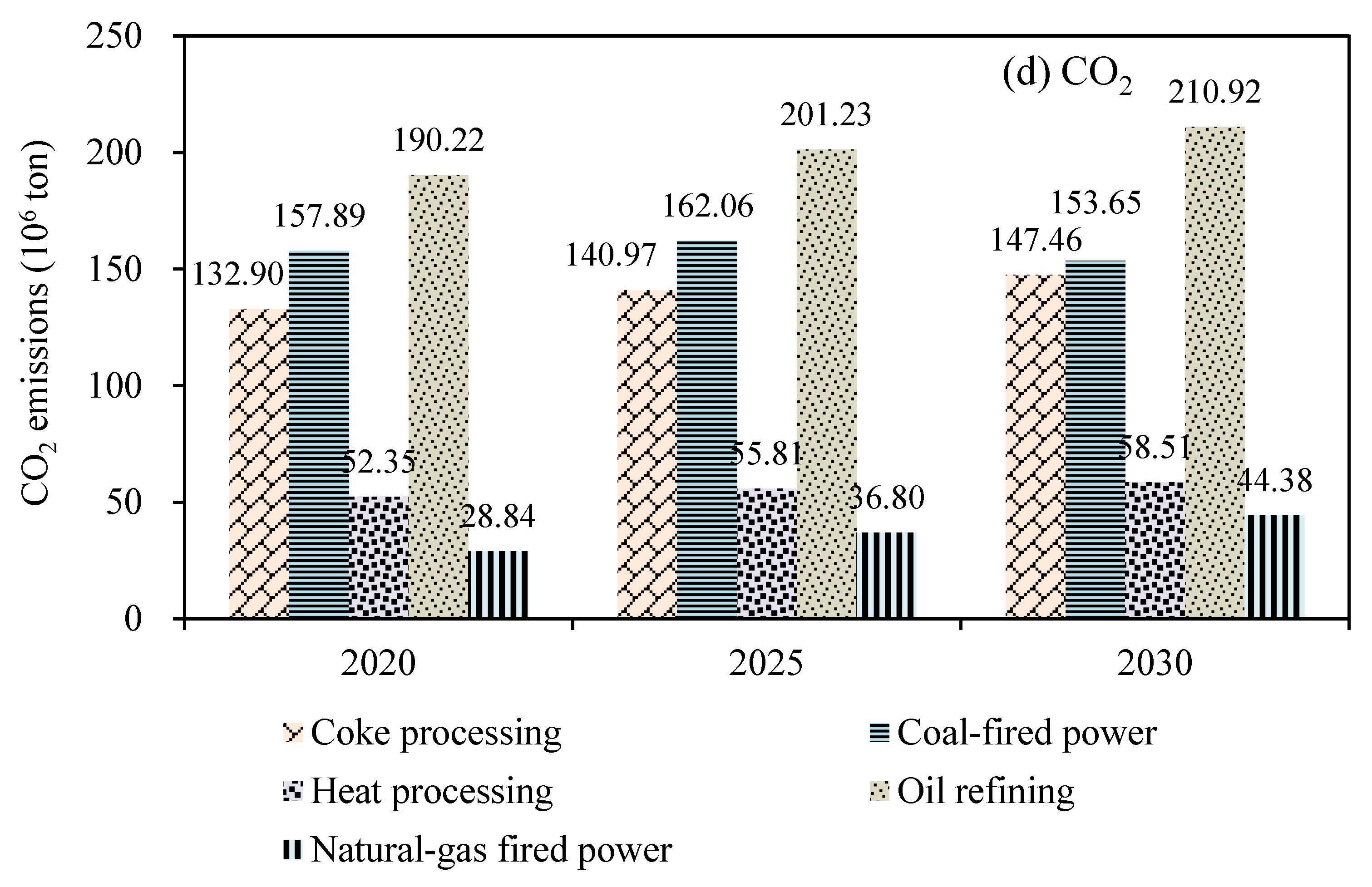
CO2 emissions. Constraints (81) to (85) represent the CO2- emissions from energy activities (i.e., coke processing, heat processing, electricity generation, and oil refining).
C O 2 K t = C F C J t · C C O 2 t
C O 2 C E t = E C O A L M t ·   C C O 2 t
C O 2 N E t = N E G M t · N C O 2 t
C O 2 H t = C F H G C t · C C O 2 t + C F H G N t · N C O 2 t
C O 2 O t = O F O I L t · O C O 2 t
where C C O 2 t is the CO2 emission factor of coal; N C O 2 t is the CO2 emission factor of natural gas; O C O 2 t is the CO2 emission factor of crude oil.
(8) The expected deviations for stochastic uncertainties. These constraints are used for capturing the risk from stochastic uncertainties.
V i t h = P P ˜ i t · Y i t h ± h = 1 H p t h P P ˜ i t · Y i t h ± + 2 θ h ; i , t , h
V C i t h = ( A ˜ i t Q i t h + B ˜ i t Z i t h ) h = 1 H p t h ( A ˜ i t Q i t h + B ˜ i t Z i t h ) + 2 θ h ; i , t , h
V i t h ± 0 ,   V C i j c t h ± 0 ;
where θ h 0 are slack variables that can achieve looser constraints; V i t h and V i j c t h are the weighted values of the expected deviations from stochastic uncertainties.
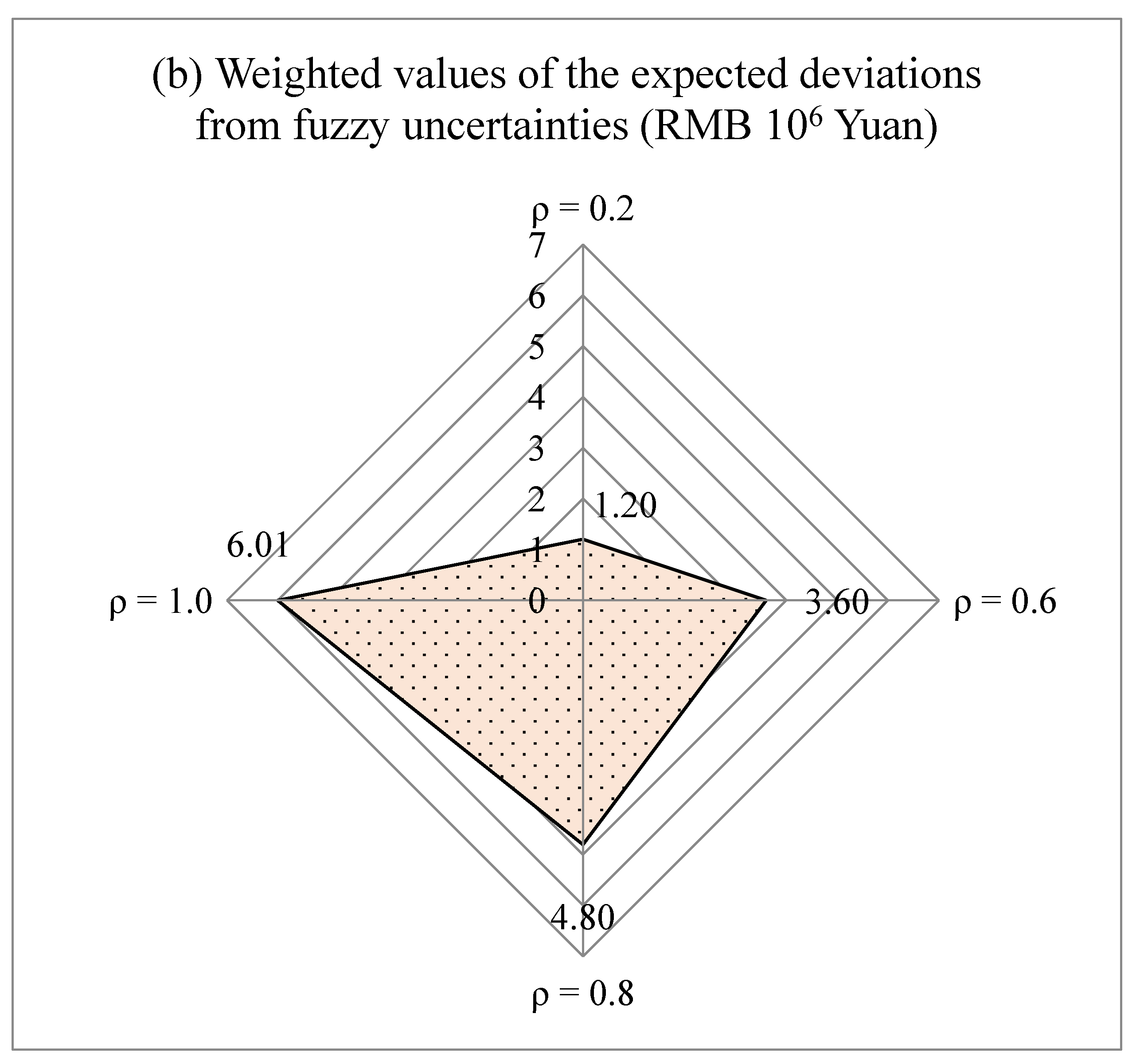
(9) The expected deviations for fuzzy uncertainties. These constraints are used for capturing the risk from fuzzy uncertainties.
V F t = ( D M C J t R ( α ) D M C J t 1 ) + ( D M H t R ( α ) D M H t 1 ) + g = 1 5 ( M A L g t R ( α ) M A L g t 1 ) + h = 1 3 [ D t h R ( α ) D t h 1 ] ; g , t , h
V F t 0
where V F t represents the positive deviation between maximum values and worst value of fuzzy parameters of right-side of constraints. D M C J t R ( α ) , D M H t R ( α ) , M A L t R ( α ) , and D t h R ( α ) are the maximum values of all potential values, i.e., D M C J t R ( α ) = sup { B | B = μ 1 ( α ) } , μ 1 is the inverse of μ . D M C J t 1 ( α ) , D M H t 1 ( α ) , M A L t 1 ( α ) , and D t h 1 ( α ) represent the possible worst values of fuzzy numbers D M C ˜ J t ( α ) , D M ˜ H t ( α ) , M A ˜ L t ( α ) , and D ˜ t h ( α ) , respectively.
(10) Non-negative constraints. This constraint assures that only positive variables are considered in the solutions, eliminating infeasibility while calculating the solution.
M A g t , E P A i t ,   H G A t ,   C F H G C t ,   C F H G N t ,   O F O I L t , C K P A t , E C O A L M t , E N G M t , E d t h , r r i t , E V E C t , Y i t h , Q i t h , Z i t h   0

3.4. Data Acquirement

The data sources of the DRSFO-EES are related references, government reports, and statistical yearbooks. The data regarding the vehicle population of the BTH region in particular was obtained from reference [38]. The annual average vehicle kilometers travelled (VKT) data were obtained from related reference [40,41,42]. Table 2 details the vehicular emission factors of China-V and China-VI [40,41,43,44,45,46,47,48]. Table 3 gives the electricity demands and representative technical data [1,23,49,50,51,52]. The electricity demands were expressed as stochastic uncertain with three probability levels (20%, 60%, and 20% corresponding to low, medium, and high levels of electricity demand, respectively). The residual capacities and operation times of the different electricity generation technologies were obtained from [49]. The CO2 and air-pollutant emission factors were acquired from related references and Intergovernmental Panel on Climate Change (IPCC) reports [2,3,53,54].

4. Results analysis

4.1. Analysis of Vehicular Emissions of BTH Region

Several policies on vehicular emission mitigation, such as the development of EVs, EV power sources and vehicular emission standards, have been proposed by the government of China. In this study, five scenarios labeled S1–S5 were designed to analyze the potentials of different emission mitigation strategies and policies for reducing vehicular emissions (NOx, HC, CO, and PM) in the BTH region. Table 4 gives the parameter settings of the different scenarios. Following is a description of each scenario:
  • S1: Without consideration of EVs, and with the local governments implementing the China V vehicular emission standard.
  • S2: With consideration of EVs, which account for 1.5% of the LDVs population. EV power sources are 100% based on coal-based power, and the China V vehicular emission standard is implemented.
  • S3: With consideration of EVs, which account for 1.5% of the LDVs population. EV power sources are based 50% on coal-based and 50% on renewable power. It is assumed that coal-based power is local coal-based power, and renewable power included wind, solar power and imported electricity. The China V vehicular emission standard is implemented.
  • S4: With consideration of EVs, which account for 1.5% of the LDVs population and with power sources based 100% on renewable energy. The China V vehicular emission standard is implemented.
  • S5: With consideration of EVs, which account for 1.5% of the LDVs population and with power sources based 100% on renewable energy. The China VI vehicular emission standard (gasoline standard) is implemented.

4.1.1. Contributions of Different Vehicle Categories to Vehicular Emissions

Numerous results were obtained by the DRSFO-EES model, and the situation of α = 0.5, ρ = 0.2, and scenario S2 is used here as an example to illustrate the optimized solutions for the EES. The rapid development of traffic systems has led to large amounts of vehicular emissions such as CO, HC, NOx, and PM. Figure 3 presents the contributions of the different vehicle categories to vehicular emissions in the BTH region over the planning periods. As indicated in Figure 3a–d, due to the sharp growth of LDVs, the total CO, NOx, HC, and PM emissions are expected to increase by 23.28%, 17.07%, 17.19%, and 22.22% over the planning periods, respectively. The results indicated that LDVs are the major contributors of CO and HC emissions, to which they contribute 65.46–73.72% and 60.15–69.15%, respectively, over the planning horizon. It is therefore necessary for local governments to limit the number of LDVs through appropriate measures and policies such as improvement of the public transit system and encouragement of the use of EVs.
Further, HDTs are the major contributor of NOx and PM, to which they are expected to contribute 67.07–63.08% and 58.58%–54.98%, respectively, between 2020 and 2030. Limiting the development of HDTs would therefore be effective for reducing vehicular NOx and PM emissions. The results also indicated that the traffic sector is set to be one of the major emitters for NOx in the BTH region. For example, the NOx emission from vehicles will account for 58.65%, 60.13%, and 61.90% of the total NOx emission (the total NOx emission includes contributions from oil refining, coke processing, heat processing, natural gas-based power, and coal-based power) in 2020, 2025, and 2030, respectively.

4.1.2. Analysis of the Impact of Traffic Policies on Vehicle Pollutants

Figure 4 shows the vehicular emissions for different scenarios and can be used to analyze the pollutant emission mitigation potential of different vehicle policies. As per the results, implementation of the stringent China VI emission standard is effective for mitigating vehicular emissions, especially CO and HC emissions. The standard is specifically projected to afford CO, HC, NOx, and PM emission reductions of 49.08%, 49.00%, 4.88%, and 0.00%, respectively, in 2020. As also indicated in Figure 4, the adoption of an EVs policy could reduce CO, NOx, HC, and PM emissions from vehicles by 25.01×10³, 1.07×10³, 4.11×10³, and 0.08×10³ ton, respectively, by 2020. However, approximately 2.6×10⁹, 3.2×10⁹, and 3.7×10⁹ kWh of electricity would have to be added by 2020, 2025, and 2030, respectively, to meet the power requirements of EVs. This implies the emission of additional air pollutants (SO2, NOx, PM, and CO2) through the increased electricity generation. Further analysis is thus required to explore the comprehensive impact of the adoption of EVs on pollutant emissions.
The sources of electricity for EVs generally include coal-based power and renewable energy. In this study, it is assumed that electricity from coal-based power was locally generated and renewable power means solar, wind power and imported electricity. Based on different power sources of EVs, there would be different impacts on the environment. Figure 5 shows the additional CO2 and air pollutant (PM, SO2, and NOx) emissions that result from the additional electricity generation required by the adoption of EVs. As can be seen, an EVs policy promises to effectively mitigate CO and HC emissions in all the scenarios. However, it increases SO2 and CO2 emissions. Moreover, no reduction in NOx and PM emissions would be achieved by the EVs policy if the power required by the EVs were entirely generated by coal-based power. Actually, in such a case, the total NOx emission would increase by 0.72×103 ton by 2020, 0.87×103 ton by 2025, and 1.32×103 ton by 2030. Conversely, if the power for EVs was generated 50% by coal-based and 50% from renewable sources, as in scenario S3, the EVs policy would reduce NOx emission by 0.17×103 ton by 2020, 0.21×103 ton by 2025, and 0.24×103 ton by 2030. If the EVs power was entirely generated from renewable sources, as in scenario S4, the policy would remarkably reduce NOx emission by 1.07×103 ton by 2020, 1.29×103 ton by 2025, and 1.49×103 by 2030. These results indicate that the vehicle-emissions could be reduced directly; but through the extra electricity generated from local region, leading to additional air-pollutants. Thus, an EVs policy should be enhanced by increasing the ratio of the needed power generated from renewable sources.

4.2. Optimized Robust Solutions For Energy and Environment Systems

4.2.1. Optimized Schemes of Energy Allocation

Figure 6 shows the optimized energy consumption of energy processing (heat processing, coke processing, and oil refining) and electricity generation (natural gas-based power and coal-based power) between period 1 and period 3. The use of natural gas is expected to substantially increase toward achieving a sustainably developed society. For example, the natural gas inputs to heat processing and natural gas-based power generation are projected to respectively increase by 47.16% (from 3.15 × 10⁹ m3 in 2020 to 4.63 × 10⁹ m3 in 2030) and 53.86% (from peak m 9.51 × 10⁹ m3 to 14.63 × 10⁹ m3) between 2020 and 2030. Crude oil input to oil refining, coal input to coke processing, and coal input to heating processing are expected gradually increase by 10.88%, 10.95%, and 3.86%, respectively, in periods 1, 2 and 3. Conversely, the coal consumption of coal-based power generation is expected to decrease by 2.69% between 2020 and 2030, specifically from 79.83 × 10⁶ ton to 77.68 × 10⁶ ton between period 1 and period 3. An appropriate energy mix can thus be effectively used to reduce coal consumption, and hence mitigate pollutant emissions.

4.2.2. Optimized schemes of electricity supply

Figure 7a shows the optimized electricity generation scheme between 2020 and 2030. The major electricity power conversion technologies in the BTH region include gas-based, coal-based, wind, and solar power. Optimized electricity generation is defined by the following equation: O E G k t h   o p t   =   W k t   o p t ±   +   Y k t h   o p t , where W k t opt ± and Y k t opt are the amounts of electricity generated in the first and second stages. Coal-based power is expected to play the dominant role, contributing what would be 259.06 × 10⁹ kWh, 265.41 × 10⁹ kWh, and 250.97 × 10⁹ kWh in periods 1, 2 and 3 (h = 3), respectively. With the implementation of a series of energy mix policies for pollutant emission mitigation, such as the “Paris Agreement” and “Chinese Action Plan of Air Pollution Prevention and Control”, the ratio of coal-based power generation would decrease from 68.79% in 2020 to 55.48% in 2030. The utilization of natural gas-based and renewable energy would rapidly develop from 2020 to 2030. Natural gas-based power, wind power, solar power and generation are projected to increase by 53.86%, 87.96%, and 266.34% over the planning horizon, contributing 22.65%, 20.44%, and 1.44%, respectively to the total power generation by 2030.
Further, the amount of locally generated electricity is insufficient for the needs of the BTH region, with approximately 36% of the consumed electricity imported from other regions. Figure 7b describes imported electricity under different electricity demand levels between 2020 and 2030. Imported electricity is expected to increase from 202.47 × 10⁹ to 254.47 × 10⁹ kWh over the planning horizon under a high electricity demand level. This indicates that imported electricity is expected to play an increasingly important role from period 1 to period 3, especially at a high demand level.

4.2.3. Optimized schemes of energy processing

Figure 8 shows the amounts of processed secondary energy (i.e., coke, heat, diesel, gasoline, fuel oil, liquefied petroleum gas, kerosene, naphtha, and tar) during periods 1 to 3. With the rapid development of society over the entire considered time, the energy processing amounts for heat, gasoline, coke, kerosene, naphtha, fuel oil, tar, and liquefied petroleum gas (LPG) are expected to respectively increase by 10.37%, 29.98%, 10.59%, 19.97%, 1.11%, 7.48%, 6.90%, and 8.84%, between 2020 and 2030.

4.2.4. Pollutant Emissions from Energy Activities

Figure 9 shows the CO2 and air pollutant (NOx, SO2, and PM) emissions from natural gas-based power generation, coal-based power generation, heat processing, coke processing, and oil refining) over the planning horizon. As can be observed, CO2, NOx, SO2, and PM emissions are expected to gradually increase by 9.37%, 5.25%, 4.43%, and, 3.59%, respectively, between 2020 and 2030. The air-pollutants emissions would approach their peak values around 2030. For example, the SO2 emission would increase by 4.14% between 2020 and 2025, and by 0.27% between 2025 and 2030, indicative of peaking around 2030. Coal-based power generation would be the major contributor of NOx, SO2, and PM emissions, respectively accounting for 36.66–33.90%, 41.89–39.03%, and 47.33–44.46% of these emissions between 2020 and 2030, with the specific contributions progressively decreasing. Coke processing would contribute 30.86–32.53%, 35.26%–37.46%, and 39.84%–42.67% of NOx, SO2, and PM emissions, respectively.
As indicated in Figure 9d, oil refining, coal-based power generation, and coke processing would be the major sources of CO2 emissions between 2020 and 2030 in BTH region, accounting for 33.83–34.30%, 28.08–24.99%, and 23.64–23.98%, respectively. In conclusion, coal-based power generation and coke processing would be the major enablers of SO2, NOx, and PM emissions reduction, while oil refining, coal-based power generation, and coke processing would be the major contributors of CO2 emission.

4.2.5. Analysis of system cost

The system costs are composed of 16 main components, namely, the costs of heat processing, coke processing, oil refining, coal input to coal-based power generation, natural gas input to natural gas-based power generation, imported electricity, first-stage of electricity generation, second-stage of electricity generation, electricity expansion, subsidy for solar power generation, subsidy for wind power generation, energy production, EVs charging piles, EVs charging stations, pollutants treatment, and risk recourse for the stochastic and fuzzy uncertainties. As shown in Figure 10, the costs of electricity generation, imported electricity, energy production, and coal input for coal-based power generation account for 30.51%, 16.90%, 16.67%, and 11.98% of the total system costs, respectively. Solar and wind power would be subsidized by the local government because their current price and technology limitations make them uncompetitive in the market. Government subsidies for wind and solar power would be RMB ¥ 40.99 × 10⁹, and RMB ¥ 6.52 × 10⁹, respectively.

5. Discussion

5.1. Analysis of Atochastic Uncertainties

In EES in the real-world, many parameters are expressed as random distribution (i.e., electricity demand, electricity generation, and electricity expansion). In this study, the TSP method was used to tackle the stochastic uncertainties. The decision variables of the electricity generation were divided into two subsets, namely, W k t opt ± and Y k t opt , which are respectively the amounts of electricity generated in the first-stage (which must be predetermined) and the second-stage (obtained after the determination of the random variables) [55]. Generally, shortages may occur if the electricity demand-levels are continuously high, and the second-stage electricity generation amount Y k t opt would be undertaken to avoid insufficient electricity supply.
In the TSP method, the final optimized electricity generation schemes were equal to W k t ± + Y k t h ± . In detail, the optimized amount of electricity generated in the first-stage is given by W k t ± = W k t + r r k t · Δ W , where r r k t denotes the decision variables, Δ W = W k t + W k t , and r r k t [ 0 ,   1 ] . Take period 1 for example, λ 11 o p t = 0.55, λ 21 o p t = 1, λ 31 o p t = 1.00, and λ 41 o p t = 1.00, indicating that the optimized electricity generation amounts for coal-based power, natural gas-based power, solar power and wind power are supposed to be (221.08 + 0.52 × 58.74) × 109, (58.41 + 1.00 ×5.00) × 109 kWh, (1.78 + 1.00 × 0.50) × 109 kWh, and (49.54 + 1.00 × 9.36) × 109 kWh, respectively. Generally, the variation of r r k t represents diverse policies of electricity generation under stochastic electricity demands. When r r k t = 0, the cost would be relatively low, although a higher penalty may have to be paid when the generated electricity does not meet the demand. On the contrary, when r r i t = 1, the cost would be higher, but accompanied by a lower risk of violating the target, and hence of incurring a lower penalty.

5.2. Analysis of Fuzzy Uncertainties

In the real world, energy price and energy demands often exhibit vagueness and ambiguity because of the subjectivity of human judgment [25]. According to FPP theory, the minimum, medium, and maximum values of these parameters are sufficient for expressing a triangular fuzzy parameter. And the proposed DRSFO-EES model can be used to effectively address the uncertainties expressed as triangular fuzzy parameter of the objectives and constraints. For FPP, the confidence level α is an indication of the manager’s violation risk attitude towards imprecise information [56,57]. In the present application of the DRSFO-EES model, four confidence levels (α = 0.5, 0.6, 0.8, and 0.9) were used to examine the impacts of different confidence levels on the EES. Generally, a higher confidence level implies a higher likelihood of satisfying the fuzzy confidence constraints, resulting in less uncertainty about the imprecise constraints. For instance, a confidence level of 0.8 indicates that the credibility of the constraint (e.g., C r { M A ˜ L g t | M A g t M A ˜ L g t } α ) is greater than or equal to 0.8. However, a higher confidence level increases the system costs. Contrarily, a lower confidence level implies a more aggressive attitude of the decision maker regarding the expected total system costs, and increases the uncertainty of the fuzzy constraints, resulting in a higher risk of violating the energy demand. Table 5 gives the optimized solution under different confidence levels α during the planning periods. As can be seen, a higher α increases the coefficients of the right-side constraints, further necessitating electricity import and increasing pollutant emission and the system costs. Vehicle ownership, heat processing, and coke processing also increase with α, all accompanied by pollutant emissions.

5.3. Risk Analysis

A robust optimization method can be effectively used to determine the associated risk from stochastic and fuzzy uncertainties. In this study, two risk recourse actions were adopted to make the model robust, which were used to capture the risks from stochastic and fuzzy uncertainties, respectively. Figure 11 presents the weighted values of the expected deviations from the stochastic uncertainties ( V T ˜ S = ρ · i = 1 I t = 1 T h = 1 H p t h ( V i t h + V C i j c t h ] ) and fuzzy uncertainties ( V T ˜ F = ρ · t = 1 3 V F t ) under different robustness levels of 0.2, 0.6, 0.8, and 1.0, respectively. ρ is a goal programming weight, through varying the ρ level, the decision makers can then control the variability of the recourse cost. Generally, a lower ρ corresponds to a lower weight value of the expected deviations and system costs, indicating an aggressive attitude of the manager regarding the system costs. However, this might be associated with a higher risk level because of the expected deviations from the uncertainties. On the contrary, a plan with a higherρwould better resist a deviation from the uncertainties of the EES. A decision with a higher robust level would thus correspond to a lower risk of system failure and higher system reliability. As results, the weighted values of the expected deviations from the stochastic and fuzzy uncertainties increased with increasing robustness level ρ. For instance, V T ˜ S would be RMB 5.17 × 10⁹ when ρ = 0.2, RMB 15.54 × 10⁹ when ρ = 0.6, RMB 20.71 × 10⁹ when ρ = 0.8, and 25.89 × 10⁹ when ρ = 1. This analysis demonstrates the trade-offs between system costs and reliability. The results enable the manager to plan with a reasonable consideration of both system costs and reliability.

6. Conclusions

In this study, a DRSFO-EES model was developed for planning an EES while considering the traffic sector, which integrates the TSP, FPP, RTSO, and RFPP methods in a single framework for the effective handling of EES uncertainties expressed as fuzzy sets and stochastic uncertainties as well as their combinations, capturing of the associated risks from the stochastic and fuzzy uncertainties, and analyzing the trade-offs between system costs and reliability. Four confidence levels (α = 0.5, α = 0.6, α = 0.8, and α = 0.9) and four robust levels (ρ = 0.2, ρ = 0.6, ρ = 0.8, and ρ = 1.0) were used for examining the impacts of uncertainties on the objective function, constraints and optimized solutions of the DRSFO-EES model.
The proposed model was applied to the EES of the BTH region in China. Following is a summary of the findings and the identified policy implications:
(1)
Limiting the numbers of LDVs and HDTs could effectively reduce vehicular emissions. LDVs are expected to be the major contributors of CO and HC emissions, and HDTs are expected to be the major contributors of NOx and PM emissions.
(2)
A EVs policy would be enhanced by increasing the ratio of power generated for EVs from renewable sources. The emission reduction effect of an EVs policy would thus be limited, especially with regard to NOx and PM emissions, if the EVs power source was entirely coal-based.
(3)
Optimizing the energy mix and developing the renewable energy can effectively reduce air-pollutant and CO2 emissions. Air-pollutant amounts of NOx, SO2, and PM emissions in the BTH region are expected to peak around 2030, because the energy mix of the study region would be transformed from one dominated by coal to one with a cleaner pattern, with vigorous development of the utilization of natural gas and renewable energy.
(4)
Enhancement of the energy utilization efficiencies of coal-based power generation, oil refining, and coke processing would effectively reduce CO2 and air-pollutant emissions. Coal-based power generation and coke processing are expected to be the major contributors of air-pollutant missions, while oil refining, coal-based power generation and coke processing would be the chief sources of CO2 emissions.
Although the DRSFO method was the first attempt for planning an EES while considering the traffic sector of the BTH region, results indicated that DRSFO-EES could: (i) explore the impacts of different vehicle policies (i.e., EVs deployment, EVs power source for EVs, and vehicular emission standards) on vehicular emissions; (ii) generate robust optimized solutions for energy allocation, oil refining, coking processing, heat processing, electricity generation and expansion, electricity importation, as well as emission mitigation under multiple uncertainties; (iii) identify the atmospheric pollution contributions of different energy activities such as coke processing, electricity generation, heat processing, oil refining, and motor vehicle operation. The proposed model could help to balance the contradiction between increasing energy demands and an increasing vehicle population, “high coal” energy systems, and the pressures of emission mitigation. Moreover, the proposed model could be applied at both city and regional scales, which would support policymakers adjusting current energy and environmental strategies in sustainable and robust ways.
However, the DRSFO-EES also has potential limitations and extensions should be addressed in future study. Firstly, the developed model, based on historical data of annual electricity demand to predict future electricity demands, does not consider the specific parameters such as hourly or seasonal electricity load curves, which may result in significant deviations from the optimized decision schemes, even in the event of electricity shortage. Thus, further study is required for considering the hourly and seasonal electricity load curves; secondly, the TSP, FPP, RTSO, and RFPP methods were combined into a single framework to formulate the DRSFO-EES model, leading to relatively high computational requirements. As a result, simplifying the calculation procedure could be required in the further study work; thirdly, the DRSFO-EES model mainly focused on economic objectives, whilst scarcely considering the trade-off between economic and environmental objectives. Therefore, further study should make improvements in the handling of multi-objective problems and better balance the tension between energy and environmental systems.

Author Contributions

C.C. proposed and calculated the DRSFO-EES model through Lingo 11, as well as analyzed the results and wrote this original manuscript; X.T.Z. and contributed in conceptualization of idea; G.H.H. contributed in supervision and revised the manuscript; Y.L. has collected the data, analyzed related data; Y.P.L. contributed in editing the manuscript.

Funding

This research was supported by the national natural science fund projects (No. 41701621, 71673022); Beijing Municipal Social Science Foundation (No. 18LJC006,17LJB004); Self-designed project of Heilongjiang Institute of Water Conservancy Science (ZN201806). The authors are grateful to the editors and the anonymous reviewers for their insightful comments and suggestions.

Conflicts of Interest

The authors declare no conflict of interest.

References

  1. Chen, C.; Long, H.L.; Zeng, X.T. Planning a sustainable urban electric power system with considering effects of new energy resources and clean production levels under uncertainty: A case study of Tianjin, China. J. Clean. Prod. 2018, 17, 67–81. [Google Scholar] [CrossRef]
  2. Chen, C.; Qi, M.Z.; Kong, X.M.; Huang, G.H.; Li, Y.P. Air pollutant and CO2 emissions mitigation in urban energy systems through a fuzzy possibilistic programming method under uncertainty. J. Clean. Prod. 2018, 192, 115–137. [Google Scholar] [CrossRef]
  3. Chen, C.; Zhu, Y.; Zeng, X.T.; Huang, G.H.; Li, Y.P. Analyzing the carbon mitigation potential of tradable green certificates based on a TGC-FFSRO model: A case study in the Beijing-Tianjin-Hebei region, China. Sci. Total Environ. 2018, 630, 469–486. [Google Scholar] [CrossRef] [PubMed]
  4. Ministry of Environment Protection of the People’s Republic of China. China’s Environmental Statistics Yearbook; China Statistics Press: Beijing, China, 2017.
  5. Guo, X.R.; Fu, L.W.; Ji, M.; Lang, J.L.; Chen, D.S. Scenario analysis to vehicular emission reduction in Beijing-Tianjin-Hebei (BTH) region, China. Environ. Pollut. 2016, 216, 470–479. [Google Scholar] [CrossRef] [PubMed]
  6. Yu, L.; Li, Y.P. A flexible-possibilistic stochastic programming method for planning municipal-scale energy system through introducing renewable energies and electric vehicles. J. Clean. Prod. 2019, 207, 772–787. [Google Scholar] [CrossRef]
  7. Odetayo, B.; MacCormack, J.; Rosehart, W.D.; Zareipour, H.; Seifi, A.R. Integrated planning of natural gas and electric power systems. Electr. Power Energy Syst. 2018, 103, 593–602. [Google Scholar] [CrossRef]
  8. Chen, J.P.; Huang, G.H.; Baetz, B.W.; Lin, Q.G.; Dong, C.; Cai, Y.P. Integrated inexact energy systems planning under climate change: A case study of Yukon Territory, Canada. Appl. Energy 2018, 229, 493–504. [Google Scholar] [CrossRef]
  9. Sahabmanesh, A.; Saboohi, Y. Model of sustainable development of energy system, case of Hamedan. Energy Policy 2017, 104, 66–79. [Google Scholar] [CrossRef]
  10. Peker, M.; Kocaman, S.A.; Kara, B.Y. A two-stage stochastic programming approach for reliability constrained power system expansion planning. Electr. Power Energy Syst. 2018, 103, 458–469. [Google Scholar] [CrossRef]
  11. Markel, E.; Sims, C.; English, B.C. Policy uncertainty and the optimal investment decisions of second-generation biofuel producers. Energy Econ. 2018, 76, 89–100. [Google Scholar] [CrossRef]
  12. Yu, L.; Li, Y.P.; Huang, G.H. Planning municipal-scale mixed energy system for stimulating renewable energy under multiple uncertainties—The City of Qingdao in Shandong Province, China. Energy 2019, 166, 1120–1133. [Google Scholar] [CrossRef]
  13. Sarkar, M.; Sarkar, B.; Iqbal, M.W. Effect of Energy and Failure Rate in a Multi-Item Smart Production System. Energies 2018, 11, 2958. [Google Scholar] [CrossRef]
  14. Wen, W.; Zhou, P.; Zhang, F.Q. Carbon emissions abatement: Emissions trading vs consumer awareness. Energy Econ. 2018, 76, 34–47. [Google Scholar] [CrossRef]
  15. Zeng, X.T.; Zhu, Y.; Chen, C.; Tong, Y.F.; Li, Y.P.; Huang, G.H.; Nie, S.; Wang, X.Q. A production-emission nexus based stochastic-fuzzy model for identification of urban industry-environment policy under uncertainty. J. Clean. Prod. 2017, 154, 61–82. [Google Scholar] [CrossRef]
  16. Gong, J.W.; Li, Y.P.; Suo, C. Full-infinite interval two-stage credibility constrained programming for electric power system management by considering carbon emissions trading. Electr. Power Energy Syst. 2019, 105, 440–453. [Google Scholar] [CrossRef]
  17. Ervural, B.C.; Zaim, S.; Delen, D. A two-stage analytical approach to assess sustainable energy efficiency. Energy 2018, 164, 822–836. [Google Scholar] [CrossRef]
  18. Simic, V. End-of life vehicles allocation management under multiple uncertainties: An interval-parameter two-stage stochastic full-infinite programming approach. Resour. Converv. Recycl. 2016, 114, 1–17. [Google Scholar] [CrossRef]
  19. Marvromatidis, G.; Orehounig, K.; Garmeliet, J. Design of distributed energy systems under uncertainty: A two-stage stochastic programming approach. Appl. Energy 2018, 222, 932–950. [Google Scholar] [CrossRef]
  20. Mohan, V.; Singh, J.G.; Ongsakul, W. An efficient two-stage stochastic optimal energy and reserve management in a microgrid. Appl. Energy 2015, 160, 28–38. [Google Scholar] [CrossRef]
  21. Bai, D.; Carpenter, T.J.; Mulvey, J.M. Making a case for robust models. Manag. Sci. 1997, 43, 895–907. [Google Scholar] [CrossRef]
  22. Chen, C.; Li, Y.P.; Huang, G.H.; Li, Y.F. A robust optimization method for planning regional-scale electric power systems and managing carbon dioxide. Electr. Power Energy Syst. 2012, 40, 70–84. [Google Scholar] [CrossRef]
  23. Chen, C.; Li, Y.P.; Huang, G.H. Interval-fuzzy municipal-scale energy model for identification of optimal strategies for energy management—A case study of Tianjin, China. Renew. Energy. 2016, 86, 1161–1177. [Google Scholar] [CrossRef]
  24. Xu, Y.; Huang, G.H.; Qin, X.S. Inexact two-stage stochastic robust optimization model for water Resources management under uncertainty. Environ. Eng. Sci. 2009, 26, 1765–1774. [Google Scholar] [CrossRef]
  25. Xu, Y.; Huang, G.H. Development of an improved fuzzy robust chance-constrained programming model for air quality management. Environ. Model Assess. 2015, 20, 533–548. [Google Scholar] [CrossRef]
  26. Govindan, K.; Cheng, T.C.E. Advances in stochastic programming and robust optimization for supply chain planning. Comput. Oper. Res. 2018, 100, 262–269. [Google Scholar] [CrossRef]
  27. Xu, Y.; Huang, G.H.; Li, J.J. An enhanced fuzzy robust optimization model for regional solid waste management under uncertainty. Eng. Optim. 2016, 48, 1869–1886. [Google Scholar] [CrossRef]
  28. Promentilla, M.A.B.; Janairo, J.J.B.; Yu, D.E.C.; Pausta, C.M.J.; Beltran, A.B.; Huelgas-Orbecideo, A.P.; Tapia, J.F.D.; Aviso, K.B.; Tan, R.R. A stochastic fuzzy multi-criteria decision-making model for optimal selection of clean technologies. J. Clean. Prod. 2018, 183, 1289–1299. [Google Scholar] [CrossRef]
  29. Jiménez, M.; Arenas, M.; Bilbao, A.; Rodriguez, M.V. Linear programming with fuzzy parameters: An interactive method resolution. Eur. J. Oper. Res. 2007, 177, 1599–1609. [Google Scholar] [CrossRef]
  30. Vahdani, B.; Razmi, J.; Tavakkoli-Moghaddam, R. Fuzzy possibilistic modeling for closed loop recycling collection networks. Environ. Model. Assess. 2012, 17, 623–637. [Google Scholar] [CrossRef]
  31. Lu, W.T.; Dai, C.; Fu, Z.H.; Liang, Z.Y.; Guo, H.C. An interval-fuzzy possibilistic programming model to optimize China energy management system with CO2 emission constraint. Energy 2018, 142, 1023–1039. [Google Scholar] [CrossRef]
  32. Pishvaee, M.S.; Razmi, J.; Torabi, S.A. Robust possibilistic programming for socially responsible supply chain network design: A new approach. Fuzzy Sets Syst. 2012, 1, 1–20. [Google Scholar] [CrossRef]
  33. Xu, Y.; Huang, G.H.; Shao, L.G. A stochastic fuzzy chance-constrained programming model for energy–environment system planning and management in the City of Beijing. Int. J. Green Energy 2017, 14, 171–183. [Google Scholar] [CrossRef]
  34. Mulvey, J.M.; Vanderbei, R.J. Robust optimization of large-scale systems. Oper. Res. 1995, 43, 264–281. [Google Scholar] [CrossRef]
  35. Ahmed, S.; Sahinidis, N.V. Robust process planning under uncertainty. Ind. Eng. Chem. Res. 1998, 37, 1883–1892. [Google Scholar] [CrossRef]
  36. Sun, L.; Pan, B.L.; Gu, A.; Lu, H.; Wang, W. Energy–water nexus analysis in the Beijing–Tianjin–Hebei region: Case of electricity sector. Renew. Sustain. Energy Rev. 2018, 93, 27–34. [Google Scholar] [CrossRef]
  37. Zhang, Z.Z.; Wang, W.X.; Cheng, M.M.; Liu, S.J.; Xu, J.; He, Y.J.; Meng, F. The contribution of residential coal combustion to PM2.5 pollution over China’s Beijing-Tianjin-Hebei region in winter. Atmos. Environ. 2017, 159, 147–161. [Google Scholar] [CrossRef]
  38. National Bureau of Statistics of the People’s Republic of China. Chinese Statistical Yearbook; China Statistics Press: Beijing, China, 2017.
  39. Chen, L.; Guo, B.; Huang, J.S.; He, J.; Wang, H.F.; Zhang, S.Y.; Chen, S.X. Assessing air-quality in Beijing-Tianjin-Hebei region: The method and mixed tales of PM2.5 and O3. Atmos. Environ. 2018, 193, 290–301. [Google Scholar] [CrossRef]
  40. Lang, J.L.; Cheng, S.Y.; Ying, W.W.; Zhou, Y.; Wei, X.; Chen, D.S. A study on the trends of vehicular emissions in the Beijing-Tianjin-Hebei (BTH) regin, China. Atmos. Environ. 2012, 62, 605–614. [Google Scholar] [CrossRef]
  41. Lang, J.L.; Cheng, S.Y.; Han, L.H.; Zhou, Y.; Liu, Y.T. Vehicular emission characteristics in Beijing-Tianjin-Hebei (BTH) region. J. Beijing Univ. Technol. 2012, 38, 1716–1723. (In Chinese) [Google Scholar]
  42. Lang, J.L.; Zhou, Y.; Cheng, S.Y.; Zhang, Y.Y.; Dong, M.; Li, S.Y.; Wang, G.; Zhang, Y.L. Unregulated pollutant emissions from on-road vehicles in China, 1999–2014. Sci. Total Environ. 2016, 573, 974–984. [Google Scholar] [CrossRef] [PubMed]
  43. Ministry of Ecology and Environmental of the People’s Republic of China. Limits and Measurement Methods for Emissions from Diesel Fuelled Heavy-Duty Vehicles (CHINA V); Ministry of Ecology and Environmental of the People’s Republic of China Press: Beijing, China, 2013. (In Chinese)
  44. Ministry of Ecology and Environmental of the People’s Republic of China. Limits and Measurement Methods for Emissions from Light-Duty Vehicles (CHINA V); Ministry of Ecology and Environmental of the People’s Republic of China Press: Beijing, China, 2013. (In Chinese)
  45. Ministry of Ecology and Environmental of the People’s Republic of China. Limits and Measurement Methods for Emissions from Diesel Fuelled Heavy-Duty Vehicles (CHINA Ⅵ); Ministry of Ecology and Environmental of the People’s Republic of China Press: Beijing, China, 2018. (In Chinese)
  46. Ministry of Ecology and Environmental of the People’s Republic of China. Limits and Measurement Methods for Emissions from Light-Duty Vehicles (CHINA Ⅵ); Ministry of Ecology and Environmental of the People’s Republic of China Press: Beijing, China, 2018. (In Chinese)
  47. Cai, H.; Xie, S.D. Determination of emission factors from motor vehicles under different emission standards in China. Acta Scientiarum Naturalium Universitatis Pekinensis 2010, 46, 319–326. (In Chinese) [Google Scholar]
  48. Li, Y.Y. Research on Total Amount of Vehicular Emissions in Beijing-Tianjin-Hebei (BTH) Region and Its Abatement Control Stratety; Tianjin University of Technology: Tianjin, China, 2015. (In Chinese) [Google Scholar]
  49. Editorial Committee of China Electric Power Yearbook; China Electric Power Press: Beijing, China, 2017. (In Chinese)
  50. Hebei Statistics Bureau. Hebei Economic Year book; China Statistics Press: Beijing, China, 2016. (In Chinese)
  51. Tianjin Statistics Bureau. Tianjin Statistic Yearbook; China Statistics Press: Beijing, China, 2016. (In Chinese)
  52. Beijing Statistics Bureau. Beijing Statistic Yearbook; China Statistics Press: Beijing, China, 2016. (In Chinese)
  53. IPCC. Coefficient of Greenhouse Gas Emissions; IPCC: Geneva, Switzerland, 2006. [Google Scholar]
  54. Li, G.C.; Sun, W.; Huang, G.H.; Lv, Y.; Liu, Z.F. An CJ. Planning of integrated energy-environment systems under dual interval uncertainties. Electr. Power Energy Syst. 2018, 100, 287–298. [Google Scholar] [CrossRef]
  55. Chen, W.T.; Li, Y.P.; Huang, G.H.; Chen, W.T.; Chen, X.; Li, Y.P. A two-stage inexact-stochastic programming model for planning carbon dioxide emission trading under uncertainty. Appl. Energy 2010, 87, 1033–1047. [Google Scholar] [CrossRef]
  56. Dai, C.; Cai, Y.P.; Ren, W.; Xie, Y.F.; Guo, H.C. Identification of optimial placements of best management practices through an interval-fuzzy possibilistic programming model. Agric. Water Manag. 2016, 165, 108–121. [Google Scholar] [CrossRef]
  57. Zhang, X.D.; Huang, G.H.; Nie, X.H. Robust stochastic fuzzy possibilistic programming for environmental decision making under uncertainty. Sci. Total Environ. 2009, 408, 192–201. [Google Scholar] [CrossRef] [PubMed]
Figure 1. Schematic overview of this study.
Applsci 09 00928 g001
Figure 2. The schematic diagram of dual robust stochastic fuzzy optimization—energy and environmental systems (DRSFO-EES).
Applsci 09 00928 g002
Figure 3. (a) CO emissions from traffic system. (b) NOX emissions from traffic system. (c) HC emissions from traffic system. (d) PM emissions from traffic system.
Applsci 09 00928 g003aApplsci 09 00928 g003b
Figure 4. Vehicular emissions from traffic systems under different scenarios.
Applsci 09 00928 g004aApplsci 09 00928 g004bApplsci 09 00928 g004c
Figure 5. Additional emissions caused by electric vehicles under different scenarios.
Applsci 09 00928 g005
Figure 6. Optimized solutions of energy input amounts for energy processing and electricity generation between 2020 and 2030. CFO represents crude oil input to oil refining; CFH represents coal input to heat processing; NFH represents natural gas input to heat processing; CFC represents coal input to coke processing; CFF represents coal input to coal-fired power; NFC represents natural gas input to coal-fired power.
Applsci 09 00928 g006
Figure 7. Optimized solutions for electricity supply of the Beijing-Tianjin-Hebei (BTH) region between 2020 and 2030.
Applsci 09 00928 g007
Figure 8. Optimized solutions for energy processing between 2020 and 2030.
Applsci 09 00928 g008
Figure 9. Pollutants and CO2 emissions from energy activities between 2020 and 2030.
Applsci 09 00928 g009aApplsci 09 00928 g009b
Figure 10. System cost over the planning periods.
Applsci 09 00928 g010
Figure 11. Weighted values of the expected deviations under different robust levels.
Applsci 09 00928 g011aApplsci 09 00928 g011b
Table 1. Previous studies related to the subject.
Ref. No.Non-Deterministic ProgrammingResearch AreaConsidering Traffic Sector
TSPRTSOFPPRFPPEnergy SystemsOthersYesNo
[5]
[17]
[18]
[19]
[20]
[21]
[22]
[23]
[24]
[25]
[26]
[27]
[28]
[29]
[30]
[31]
[32]
Note: TSP, two-stage stochastic programming; RTSO. robust two-stage stochastic optimization; FPP, fuzzy possibilistic programming; and RFPP, robust fuzzy possibilistic programming.
Table 2. Vehicular emission factors with different emissions standards (mg/km•unit).
CONOXHCPM
HDVChina-Ⅴ300 4610 35 100
China-Ⅵ300 4610 35 100
LDVChina-Ⅴ1400 60 230 5
China-Ⅵ700 35 115 5
LDTChina-Ⅴ5800 60 1200 5
China-Ⅵ2900 35 600 5
HDTChina-Ⅴ200 3530 35 100
China-Ⅵ200 3530 35 100
OtherChina-Ⅴ2750 150 855 20
China-Ⅵ2750 150 855 20
Table 3. Electricity demand and technological data.
Period
Period 1Period 2Period 3
Electricity demand (109 kWh)
Low demand level[517.71, 537.71, 557.71][553.82, 573.82, 593.82][594.67, 614.67, 634.67]
Medium demand level[547.25, 567.25, 587.25][595.73, 615.73, 635.73][636.18, 656.18, 676.18]
High demand level[559.07, 579.07, 599.07][646.05, 666.05, 686.05][686.87, 706.87, 726.87]
Electricity generation target (109 kWh)
Coal-fired power[221.07, 279.81][213.27, 268.01]208.93, 269.50]
Gas-fired power[58.41, 63.41][76.91, 80.91][91.88, 95.88]
Wind[40.19, 49.55][45.79, 56.48][51.01, 61.94]
Solar power[1.20, 1.70][3.20, 3.60][5.99, 6.22]
Energy consumption amounts per unit of electricity production
Coal (ton of SCE/103 kWh)30.50 30.50 30.50
Natural gas (m3/103 kWh)142.80 142.80 142.80
Coal consumption amounts per unit of coke processing (ton of SCE/ton)
1.35 1.35 1.35
Energy consumption amounts for unit of heat processing (ton of SCE/109 kJ)
36.00 36.00 36.00
Table 4. Parameter settings of scenarios.
Vehicular Emissions StandardsThe Proportion of EVsPower Sources for EVs
S1China Ⅴ0%
S2China Ⅴ1.50%100% coal-fired power based
S3China Ⅴ1.50%50% coal-fired power based, 50% renewable energy based
S4China Ⅴ1.50%100% renewable energy based
S5China Ⅵ1.50%100% renewable energy based
Table 5. (a) Optimized solutions under different α levels in 2020.
α = 0.5α = 0.6α = 0.8α = 0.9
Traffic system and its relative pollutants
Vehicle ownership (106)22.11 22.34 22.80 23.03
CO emissions (103 ton)2534.02 2561.58 2616.70 2644.26
NOX emissions (103 ton)679.66 685.44 696.98 702.75
HC emissions (103 ton)452.69 457.67 467.62 472.59
PM emissions (103 ton)22.09 22.28 22.67 22.86
Heat processing (1012 kJ)
707.31 708.31 710.31 711.31
Coke processing (106 ton)
69.61 70.11 71.11 71.61
Import electricity amounts (109 kWh, h = 1 )
161.10 163.10 167.10 169.10
Air pollutants and CO2 from energy processing and electricity generation (103 ton)
SO2 emissions667.86 669.95 674.12 676.20
NOX emissions476.67 479.17 484.17 486.67
PM emissions83.92 84.18 84.69 84.95
CO2 emissions560593.92 564482.45 572259.52 576148.05
Table 5. (b) Optimized solutions under different α levels in 2025.
α = 0.5α = 0.6α = 0.8α = 0.9
Traffic system and its relative pollutants
Vehicle ownership (106)26.16 26.39 26.84 27.07
CO emissions (103 ton)2886.63 2914.19 2969.31 2996.87
NOX emissions (103 ton)754996.10 760.77 772.31 778.09
HC emissions (103 ton)510.96 515.93 525.88 530.86
PM emissions (103 ton)24.75 24.94 25.33 25.52
Heat processing (1012 kJ)
748.38 749.38 751.38 752.38
Coke processing (106 ton)
73.84 74.34 75.34 75.84
Import electricity amounts (109 kWh, h = 1 )
164.89 166.89 170.89 172.89
Air pollutants and CO2 from energy processing and electricity generation (103 ton)
SO2 emissions689.20 691.28 695.45 697.53
NOX emissions497.49 499.95 504.85 507.30
PM emissions87.16 87.41 87.93 88.18
CO2 emissions594920.14 598809.23 606587.42 610476.51
Table 5. (c) Optimized solutions under different α levels in 2030.
α = 0.5α = 0.6α = 0.8α = 0.9
Traffic system and its relative pollutants
Vehicle ownership (106)29.69 29.92 30.38 30.61
CO emissions (103 ton)3127.77 3155.33 3210.45 3238.01
NOX emissions (103 ton)819.79 825.56 837.11 842.88
HC emissions (103 ton)547.42 552.40 562.35 567.32
PM emissions (103 ton)27.01 27.21 27.59 27.78
Heat processing (1012 kJ)
780.64 781.64 783.64 784.64
Coke processing (106 ton)
77.24 77.74 78.74 79.24
Import electricity amounts (109 kWh, h = 1)
194.72 195.44 196.88 197.60
Air pollutants and CO2 from energy processing and electricity generation (103 ton)
SO2 emissions688.19 690.27 694.44 696.52
NOX emissions501.10 503.75 509.05 511.70
PM emissions86.79 87.05 87.56 87.81
CO2 emissions612669.67 617113.59 626001.42 630445.34

