The Virial Effect—Applications for SF₆ and CH₄ Thermal Plasmas

Abstract

A tool based on the mass action law was developed to calculate plasma compositions and thermodynamic properties for pure gases and mixtures, assuming a local thermodynamic equilibrium for pressures of up to 300 bar. The collection of the data that was necessary for tool calculation was automated by another tool that was written using Python, and the formats for the model were adapted directly from the NIST and JANAF websites. In order to calculate the plasma compositions for high pressures, virial correction was introduced. The influences of the parameters that were chosen to calculate the Lennard–Jones (12-6) potential were studied. The results at high pressure show the importance of virial correction for low temperatures and the dependence of the dataset used. Experimental data are necessary to determine a good dataset, and to obtain interaction potential. However, the data available in the literature were not always provided, so they are not well-adapted to a large pressure range. Due to this lack, the formulation provided by L. I. Stiel and G. Thodos (Journal of Chemical and Engineering Data, vol. 7, 1962, p. 234–236) is a good alternative when the considered pressure is not close to the critical point. The results may depend strongly on the system studied: examples using SF₆ and CH₄ plasma compositions are given at high pressure.

1. Introduction

The calculation of plasma compositions under the assumption of local thermal equilibrium (LTE) is necessary to determine the thermodynamic properties and the transport coefficients that are needed for magneto-hydrodynamic models of thermal plasma processes and systems as circuit breakers, plasma torches, or thermal engines. These compositions are also necessary as initial equilibrium states for chemical kinetic studies and to determine departures from chemical equilibrium.

In the literature, three methods are mainly used to calculate the evolution of species densities with temperature and pressure in thermal plasmas: the Gibbs free enthalpy minimization [1], the mass action law method [2,3], and the collisional radiative model. Based on these methods, numerous papers have reported chemical plasma compositions for pure gases and mixtures, with or without the LTE assumption [2,4,5,6,7,8,9,10,11,12,13,14,15,16].

Nevertheless, in most of these papers, even at high pressure (>30 bar), only the first-order Debye–Hückel correction is taken into account [2,17]. Although this correction is necessary at high temperatures to consider the Coulombic interactions between the charged particles and others, it is not sufficient for low temperatures (around 300 K), where molecule interactions are important. Under these conditions, it is necessary to correct the perfect gas behavior by considering virial pressure correction. However, in the thermal plasma community, only a few authors have considered this correction at high pressures [4,6,9,14].

The virial pressure correction can be developed over several orders, named virial coefficients. They can be obtained experimentally ([18], for instance) by deducing them from measurements of the mass density, viscosity, or, in some cases, sound velocity [19,20] or by theoretical calculation using intermolecular interaction potentials [18,21,22]. In the literature, we can find that, for some gases, the second and sometimes the third coefficients are given as a function of the temperature [19,22,23,24,25,26]. These data are very dependent on the pressure and temperature of the gas, and they are not valid for a large range of temperatures and pressures. The densities of the species, and the mass density of the gases depend very strongly on the applied dataset. This mass density has a direct effect on convection modeling for its applications.

In our research fields, at high pressures, we are particularly focused on three topics:

-

the plasma behavior in high-voltage circuit breakers (HVCBs) [27,28,29], where pressures in heating volumes can reach bar values of several tens;

-

hydro–electro formation and hydraulic fracturing using an electric arc in water [30];

-

the combustion of methane in thermal gas engines [31].

For each of these topics, the pressure considered and the gases used are different, and they include, within a high-pressure range, SF₆ for the first application, H₂O for the second, and mixtures of air and CH₄ for the third.

In the case of HVCB, some compositions and thermal properties are available in the literature; nevertheless, a complete databank for describing the current cutoff from the initial pressure to the one obtained during the high-current phase is not given, and authors seem to use the same parameters to calculate the Lennard–Jones potential for the entire pressure range [14,32,33]. This problem is the same for the case of hydro–electro formation and hydraulic fracturing: little data is available for H₂O, and only few details on the parameters that are used to calculate the Lennard–Jones potential are given. For engine applications, we did not find data related to air–CH₄ mixtures in the literature. Therefore, papers from the literature generally consider pure air, and pressure corrections are not taken into account [34,35,36].

In the first part of this paper, the method that was used to calculate the plasma composition is presented. The different equations based on the mass action law, neutrality, conservation of nuclei, and pressure law, used for determining the species densities, are given. The validation of the developed tool is presented with regard to some plasma compositions at atmospheric pressure. In the second part, the importance of the parameters that were used for determining the interaction potential for virial correction is presented. These parameters can be obtained from experimental data, or from a theoretical approach. The two methods are discussed, and they are applied to a mass density calculation. Finally, the plasma compositions of SF₆ and CH₄ are calculated at high pressures.

2. Equations and Methods

2.1. Partition Functions

Whatever the method used to calculate the compositions, partition functions are necessary. Indeed, they are the link between the microscopic and macroscopic properties of the system. For each species, the total partition function $Q_{tot}^{vol}$ can be calculated from Equation (1):

$$Q_{tot}^{vol}\left(T\right)={\left(\frac{2.\pi .m.k_B.T}{h^2}\right)}^{\frac{3}{2}}.Q_{int}.\left(e^{-\frac{E_0}{k_B.T}}\right)$$

(1)

where

-

m is the mass of the species;

-

k_B is the Boltzmann constant;

-

T is the temperature;

-

h is Planck’s constant;

-

E₀ is the energy of formation.

The first term of this equation corresponds to the translation partition function Q_trans. Q_int is the internal partition function, taking into account the vibrational, electronic, and nuclear partition functions. The last term takes into account the chemical energy that is needed for the formation of the particle. This expression differs for each species, due to their specific masses, from the internal partition function and the energy of formation. This last variable can be obtained from the JANAF table [37], which directly provides the value of the formation enthalpy ∆H_f for each species, which in most cases is estimated at absolute zero temperature.

2.1.1. The Internal Partition Function of Monoatomic Species

For species with only one atom, the internal partition function is given by Equation (2):

$$Q_{int}\left(T\right)={\displaystyle \sum }_i^{i_{max}}{g}_i.e^{-\frac{E_i}{k_B.T}}$$

(2)

where

-

g_i is the statistical weight of an electronic level i, given by g_i = 2.J + 1, where J is the angular momentum;

-

E_i is the energy of the electronic level i;

-

i_max is the limitation of the summation over the electronic levels, to avoid the divergence of the summation at high temperatures. The limit of the summation is the energy of ionization E_ion, which is reduced by the lowering of the ionization potential ΔE (i_max ≤ E_ion − ΔE). The lowering of the ionization potential (Equation (3)) is introduced in order to limit the number of electronic energy levels that are considered in the sum (Equation (2)), due to the electric and electromagnetic field effects created by the charged particles. This can be estimated from the Debye–Hückel formula (Equation (3)):

$$\Delta E=\frac{\left(Z+1\right).e^2}{4.\pi .{\epsilon }_0.{\lambda }_D} \left(eV\right)$$

(3)

where

-

Z is the electrical charge of the considered species;

-

e is the electrical charge of the electron;

-

ε₀ is the vacuum permittivity;

-

λ_D is the Debye length, given by Equation (4):

$${\lambda }_D=\sqrt{\frac{{\epsilon }_0.k_B.T}{e^2.\left(n_e+{\sum }_{i\ne e}{Z}_i^2.n_i\right)}}$$

(4)

where n_e is the electronic density, and n_i is the density of each species.

The various data on the energy levels, and the angular momentum for the calculation of the statistical weights of the considered levels, were extracted from the NIST database [38].

2.1.2. The Internal Partition Function for Molecules

For molecules, the internal partition function can be obtained from Equation (5), by using the spectroscopic data available in the JANAF database [37], and especially the free Gibbs energy and the enthalpy.

$$Q_{int}\left(T\right)=\frac{P_r}{k_B.T}{\left(\frac{h^2}{2.\pi .m.k_B.T}\right)}^{\frac{3}{2}}exp\left[\frac{1}{N_a.k_B}\left(\frac{{\left[H\left(0\right)-H\left(T_r\right)\right]}_{JANAF}}{T}-{\left[\frac{G-H\left(T_r\right)}{T}\right]}_{JANAF}\right)\right]$$

(5)

where

-

T_r and P_r are the temperature and pressure, respectively, of the reference in the JANAF database;

-

N_a is the Avogadro constant;

-

H(0) − H(T_r) represents the enthalpy at absolute zero;

-

[G − H(T_r)]/T is the Gibbs energy, which must be known for each temperature that is considered.

For the electrons, the internal partition function is constant and equal to 2.

2.2. The Equation for the Calculation of the LTE Plasma Composition

In this work, to calculate the plasma composition, we used the mass action law (Equation (6)) with the method proposed by Godin [2,3]. This method is a generalization of the Saha and Guldberg–Waage laws, and enables a fast solution for the system of equations.

$${\displaystyle \prod }_i^N{\left(n_i\right)}^{v_i}={\displaystyle \prod }_i^N{\left(Q_{tot, i}^{vol}\right)}^{v_i}$$

(6)

where n_i represents the densities of the species i, ν_i is the stoichiometric coefficients of the reaction (cf. Section 2.2.4), $Q_{tot,i}^{vol}$ is the total partition function (Equation (1)), and N is the number of species considered in the plasma.

The composition calculation can then be divided into several steps, described below.

2.2.1. Choices of Elements and Chemical Species

The chemical elements are the basic components. When an ionized gas is described, the electric charge needs to be considered and added to the list of the basic components. The chemical species are constituted of one or several of these basic components. For instance, the oxygen atom is the basic component of several chemical species, such as O, O⁺, O⁻, O₂, and O₂⁺.

Of course, the element and species choices depend on the plasma of interest. The only limit is the availability of the species data in the NIST [38] and JANAF [37] databases for the internal partition functions. In order to properly differentiate the basic components and the chemical species, two parameters, M and N, are defined. M is the number of chemical (or basic) elements, and N is the number of chemical species, with M ≤ N.

2.2.2. The Composition Matrix

Once defined as M elements and N species, the composition matrix can be built with elements C_j,i. Its dimension is N × M. This matrix links the chemical species with the basic elements. An example is shown in Equation (7), for plasma composed of dinitrogen and dioxygen.

$$\begin{array}{cc}& \hspace{1em}\begin{array}{ccc}N& O& charge\end{array}\hfill \\ \hfill C=& \left(\begin{array}{c}\begin{array}{ccc}1& 0& 0\\ 1& 0& 1\\ 2& 0& 0\end{array}\\ \begin{array}{ccc}1& 1& 0\\ 0& 1& 0\\ 0& 1& 1\end{array}\\ \begin{array}{ccc}0& 2& 0\\ 1& 2& 0\\ 0& 0& -1\end{array}\end{array}\right)\begin{array}{c}\begin{array}{c}\begin{array}{c}N\\ N^{+}\end{array}\\ N_2\\ NO\end{array}\\ O\\ \begin{array}{c}{O}^{+}\\ O_2\\ \begin{array}{c}N{O}_2\\ e^{-}\end{array}\end{array}\end{array}\}Chemicalspecies\hfill \end{array}.$$

(7)

2.2.3. The Chemical Base

The chemical base is a subsection of chemical species from which it is possible to express the other species that are not present in the base matrix, but which can be created by chemical processes. This introduces the concept of the base matrix B, and the out-of-base matrix B*. Their coefficients can be obtained from the composition matrix by Equation (8):

$$\{\begin{array}{c}{B}_{k,i}=C_{k,i}\\ B_{j,i}^{\ast }=C_{j,i}\end{array}\hspace{1em}\hspace{1em}with\hspace{1em}\hspace{1em}\{\begin{array}{c}i,kϵ\left\{1,M\right\}\\ jϵ\left\{1,N-M\right\}\end{array}.$$

(8)

In order to choose the chemical species of the base, some specific conditions have to be verified for each temperature step:

-

The densities of the species in the base matrix must be the highest densities.

-

The species of the base matrix must be independent, in order to avoid |B| = 0 (the null determinant).

-

The species that are present at very low densities must not be included in the base matrix.

For that, at the beginning of the calculation, the densities of the base species must be evaluated. This estimation depends greatly on initial temperature and on the given pressure. For instance, for the composition matrix proposed in Equation (7), the estimation of the base matrix, starting from T = 30 kK and P = 1 bar, is given in Equation (9):

$$\begin{array}{cc}& \begin{array}{ccc}N& O& charge\end{array}\hfill \\ \hfill B=& \left(\begin{array}{ccc}1& 0& 1\\ 0& 1& 1\\ 0& 0& -1\end{array}\right)\begin{array}{c}{N}^{+}\\ O^{+}\\ e^{-}\end{array}\}Species of the base\hfill \end{array}.$$

(9)

The other species in the composition matrix (Equation (7)) that are not included in matrix B (Equation (9)) are used to constitute the out-of-base matrix B*.

2.2.4. The Reaction Coefficient

The reaction coefficient matrix ν is used to link the species from the base to those that are out of the base. Its dimension is (N − M) × M, and its expression is given in Equation (10):

$$B^{\ast }=v.B\iff B_{j,i}^{\ast }={\displaystyle \sum }_{k=1}^M{v}_{j,k}.B_{k,i}$$

(10)

where k is the number of species of the base, and j is the number of out-of-base species.

From the concept of the reaction matrix coefficient, it is possible to obtain all of the chemical processes, creating out-of-base species from the base ones.

2.2.5. Conservation Equations

For closing the system, several equations of conservation are used.

-

Conservation of nuclei:

$${\epsilon }_j{\displaystyle \sum }_{i=1}^N{n}_i.C_{i,k}={\epsilon }_k{\displaystyle \sum }_{i=1}^N{n}_i.C_{i,j}\hspace{1em}\hspace{1em}where j,k\{\begin{array}{c}ϵ \left\{1,M-1\right\}\\ \ne charge\end{array}$$

(11)

with the atomic proportion ε.

-

Electric neutrality:

$${\displaystyle \sum }_{i=1}^N{n}_i.Z_i=0$$

(12)

where Z_i is the electric charge of the species i (which can be directly expressed from C_{i, charge}).

- Pressure conservation:

The plasma pressure P is determined by the Dalton law (the perfect gas law) with Debye–Hückel, and with virial correction for real fluids:

$$P={\displaystyle \sum }_{i=1}^N{n}_i.k_b.T+\Delta P_{Debye}+\Delta P_{virial}$$

(13)

where

-

ΔP_Debye is the Debye–Hückel pressure correction:

$$\Delta P_{Debye}=-\frac{k_b.T}{24.\pi .{\lambda }_D^3};$$

(14)

-

ΔP_virial is the virial pressure correction. For its calculation, several coefficients describing the difference in behavior between real fluids and perfect gases are needed. Taking into account the second- and third-order corrections, the virial pressure correction is given in Equation (15):

$$\Delta P_{virial}=k_B.T.B\left(T\right).{\left({\displaystyle \sum }_{i=1}^N{n}_i\right)}^2+k_B.T.C\left(T\right).{\left({\displaystyle \sum }_{i=1}^N{n}_i\right)}^3$$

(15)

where B(T) and C(T) are the second and third virial coefficients, respectively, and they depend on the temperature. The methods to obtain them are described in Section 3 of this paper (cf. Section 3 « virial coefficient »).

More generally, all conservation equations can be written in the form given in Equation (16):

$${\left\{{\displaystyle \sum }_{i=1}^N{A}_{l,i}.n_i=A_l^{°}\right\}}_{l=1}^M$$

(16)

where A_l,i and $A_l^{°}$ are the coefficients of the conservation equation l for species i. A summary of all of these equations is given in

Table 1. Conservation coefficients.

Conservation Equation	Al,i	${\mathit{A}}_{\mathit{l}}^{\mathit{o}}$	Number of Equations
Atomic nuclei	${\epsilon }_j{C}_{i,k}-{\epsilon }_k{C}_{i,j}$	0	M-2
Electric neutrality	$C_{i,charge}$	0	1
Pressure	1	$\raisebox{1ex}{$\left(P-\Delta P\right)$}\!\left/ \!\raisebox{-1ex}{$kT$}\right.$	1

.

2.2.6. The Equation for Out-of-Base Species Density

The general equation for the out-of-base densities $n_{b_j}^{\ast }$, depending on the base densities $n_{b_i}$, and the total partition functions of the base ($Q_{b_i}$) and the out-of-base ($Q_{b_j}^{\ast }$) species is given in Equation (17):

$${\left\{n_{b_j}^{\ast }=Q_{b_j}^{\ast }.exp\left({\displaystyle \sum }_{i=1}^M{v}_{j,i}.\left[ln\left(n_{b_i}\right)-ln\left(Q_{b_i}\right)\right]\right)\right\}}_{j=1}^{N-M}.$$

(17)

2.2.7. Numerical Methods and System of Equations

As the equation system is strongly nonlinear, a linearization algorithm based on the Newton Raphson iterative method is derived, using Equations (18)–(21):

$${\displaystyle \sum }_{i=1}^M{J}_{l,i}.\delta n_{b_i}=-R_l\hspace{1em}\iff \hspace{1em}J.\delta n=-R$$

(18)

$$R_l=-A_l^{°}+{\displaystyle \sum }_{i=1}^M{A}_{l,b_i}.n_{b_i}+{\displaystyle \sum }_{j=1}^{N-M}{A}_{l,b_j^{\ast }}.n_{b_j^{\ast }}$$

(19)

$$\begin{gathered} J_{l,i}=A_{l,b_i}+\frac{1}{n_{b_i}}{\displaystyle \sum }_{j=1}^{N-M}{A}_{l,b_j^{\ast }}.n_{b_j^{\ast }}.v_{j,i} \\ i\mathrm{and}l\mathsf{ϵ}\{1,M\} \end{gathered}$$

(20)

$$n_{b_i}=n_{b_i}+\delta n_{b_i}$$

(21)

where J_l,i is the Jacobian matrix of the system, R_l represents the residuals of the matrix, and $\delta n_{b_i}$ is the correction applied on the densities at each iteration. The convergence criterion is given in Equation (22), with a convergence threshold ε = 10⁻¹⁰ [2].

$${\left\{\frac{\left|R_l\right|}{Max{\left|\left\{A_{l,i}{n}_i\right\}\right|}_{i=1}^N} \epsilon \right\}}_{l=1}^M.$$

(22)

2.3. Automatization of the Tool

The calculation of the composition requires a large amount of information, such as the information required for the determination of the partition functions for each species, the virial coefficient, the considered pressure, and the temperature range or temperature step.

2.3.1. Data from the NIST and JANAF Tables

To simplify the searching and formatting of the data available in the NIST and JANAF tables, software was developed using Python. This enables all of the required data for the species of the chosen composition to be concatenated and formatted automatically. In the case of the data originating from the NIST [38], the added parameters for each species, complementing the different energy levels and angular momentums, are as follows:

-

the name of the species, for a link between the initialization file and the data file;

-

the energy of formation, needed for the calculation of the total partition function;

-

the energy of ionization that is used in order to satisfy the limit condition of Equation (2);

-

the units for the energy levels, depending on the extracted data (in cm⁻¹ or in eV);

-

the number of energy levels to consider, up to the ionization of the considered species;

-

the mass of the considered species.

For data from the JANAF database [37], two parameters are added: the name of the species and the mass. We have collected 296 chemical species, which can be used for calculating compositions containing carbon (C), hydrogen (H), oxygen (O), nitrogen (N), sulfur (S), fluorine (F), argon (Ar), helium (He), copper (Cu), and iron (Fe). All kinds of particles have been taken into account in this databank: atoms, molecules, positive and negative ions, and molecular ions.

2.3.2. The Initialization File

This file is very important, as it contains all of the necessary parameters for determining the densities of the species. It generally contains the following:

-

the number of gases considered in the composition.

-

the name(s) of the gas(es) in the composition (for instance, SF₆, N₂, and O₂, Ar, and Cu, etc.).

-

the molar fraction of each gas in the melt (the sum of all of the fractions must equal unity; for example, it could be 1 SF₆, 0.7885 N₂ and 0.2115 O₂, or 0.8 Ar and 0.2 Cu, etc.);

-

the number of atoms and species that come from the gas mixture, in order to define M and N (cf. Section 2.2.1);

-

the names of the species in the plasma;

-

the atomic proportions of each atom/nucleus for the considered mixture (for example, 100% SF₆: 1 S and 6 F; 78.85% N₂ and 21.15% O₂: (0.7885 × 2) N and (0.2115 × 2) O);

-

the considered pressure;

-

the temperature range and the temperature step of the results.

2.4. Results and Discussion

In order to validate our tool, we compared our results with two examples found in the literature at atmospheric pressure:

-

Case 1: pure argon;

-

Case 2: air with 78.084% N₂, 20.946% O₂, 0.036% CO₂, and 0.934% Ar.

In order to properly compare the results with the literature, we considered the same species (

Table 2. Chemical species considered for argon and air plasma compositions.

Gas	Chemical Species
Argon	Ar, Ar +, Ar +2, Ar +3, e−.
Air	N, N+, N+2, O, O+, O+2, O−, C, C+, C+2, C−, Ar, Ar+, Ar+2, N2, N2+, NO, NO+, O2, O2+, C2, CO, N2O, NO2, CO2, e−.

) reported by authors of past studies.

The composition obtained from our tool in Case 1 is shown with those of three other studies [2,11,16] in Figure 1. For the air plasma, our results were compared with the calculation of André [5], and are plotted in Figure 2 and Figure 3 (Figure 2 shows the atomic and ionic species, and Figure 3 shows the molecular species).

In the two cases (Ar and Air), a good agreement could be observed. At low temperatures, the neutral species were dominant. When the temperature increased, we observed different types of processes. In the case of argon, the ionization of the atoms and the simultaneous apparition of electrons occurred. In the case of air, we noted the dissociation of the molecules, the recombination processes, the apparition of electrons, and the ionization of atoms, but also the electronic attachments. Nevertheless, for some species, some of the results displayed differences between the literature and our calculations. These were generally due to the sources used for the internal partition function of each species. In Figure 1, the results from Godin [2] are based on the data available from Drawin & Felenbok [39]. In this database, the internal partition functions are given versus temperature, with values of the lowering of ionization potential. For the results of Rat [16], the source was not given, but the shift in argon atom density observed at high temperature could be due to the fact that the Ar⁺³ ion was not taken into account by this author. For the air composition, the partition functions calculated by André [5] were determined from data in the literature [37,38,39]. Furthermore, his calculation method was different from ours, as he used the minimization of Gibbs free energy.

Although most papers from the literature used tabulated values for the partition functions, we chose to calculate them from the available data of the NIST database [38] for monoatomic species, and from the JANAF database [37] for molecules.

By using our tool, the LTE compositions of air and argon plasmas were calculated at P = 1 bar. The choices for the temperature range and of the considered species were made with the aim of assisting with the comparison of our results against the works of other authors. The results validate our tool for atmospheric pressure.

3. Virial Coefficients

The tool presented in this study is also aimed at determining initial compositions for kinetic studies, in applications where the pressure can reach bar values of several tens. The developments, taking into account the pressure correction, are now presented. Virial coefficients are parameters that are used to describe the real behavior of a fluid. For this description, the second- (B(T)) and third-(C(T)) order coefficients could be used, and they were expressed using intermolecular potential:

$$B\left(T\right)=-2.\pi .N_a.\underset{0}{\overset{\infty }{{\displaystyle \int }}}f\left(r_{12}\right).r_{12}^2.d{r}_{12}$$

(23)

$$C\left(T\right)=-\frac{8.{\pi }^2.N_a^2}{3}.\underset{0}{\overset{\infty }{{\displaystyle \int \int \int }}}f\left(r_{12}\right).f\left(r_{13}\right).f\left(r_{23}\right).r_{12}.r_{13}.r_{23}.d{r}_1.d{r}_2.d{r}_3$$

(24)

where $f\left(r_{ij}\right)=\exp \left[-\frac{u\left(r_{ij}\right)}{k_B.T}\right]-1$ is the Mayer function, $u\left(r_{ij}\right)$ is the potential for interactions between two molecules, and r_ij are the coordinates of molecules i, relative to molecule j.

For a mixture, the virial coefficients can be expressed by Equations (25) and (26):

$$B{\left(T\right)}_{mixture}={\displaystyle \sum }_{i=1}^m{\displaystyle \sum }_{j=1}^m{B}_{ij}\left(T\right).x_i.x_j$$

(25)

$$C{\left(T\right)}_{mixture}={\displaystyle \sum }_{i=1}^m{\displaystyle \sum }_{j=1}^m{\displaystyle \sum }_{k=1}^m{C}_{ijk}\left(T\right).x_i.x_j.x_k$$

(26)

where

-

m is the number of gas for mixing;

-

x_i, x_j, and x_k are the respective molar fractions of species i, j, and k;

-

B_ij is the binary interaction parameter;

-

C_ijk is the ternary interaction parameter.

3.1. The Lennard–Jones Potential

For calculating the virial coefficients, several kinds of intermolecular potentials can be used, depending on the study [6,18,40,41,42]. Nevertheless, obtaining the third-order coefficient requires the calculation of a triple integration on the potential. In the literature, the expression of this integral is only given for a hard-sphere potential, a square-shaped potential, and the Lennard–Jones (12-6) potential [18]. This last approach seems to be the best at properly describing inter-particle interactions, and it is used in this paper.

3.1.1. Expression of the Potential

The Lennard–Jones (LJ) potential derives from the Mie potential, assuming that n = 12 and m = 6. The number 12 corresponds to the repulsive index at short distances, and 6 to the attractive index, based on Van der Waals interactions. This shape of the potential is very commonly used by other authors [13,18,43,44] for describing particle interactions in pure gas and mixtures. This potential is given by

$$u\left(r\right)=4.\epsilon .\left[{\left(\frac{\sigma }{r}\right)}^{12}-{\left(\frac{\sigma }{r}\right)}^6\right]$$

(27)

where r is the distance between two atoms.

With the LJ potential, Hirschfelder [18] proposed the use of reduced amounts of data expressed with hard-sphere potential b₀ (Equations (28) and (29)). This approach has been validated by this author for the second and third virial coefficients for several species:

$$B\left(T\right)=b_0.B^{\ast }\left(T^{\ast }\right)$$

(28)

$$C\left(T\right)=b_0^2.C^{\ast }\left(T^{\ast }\right)$$

(29)

where B*(T*) and C*(T*) are reduced values of, respectively, the second and third virial tabulated coefficients versus the reduced temperature T* given in Equation (30):

$$T^{\ast }=\frac{k_B.T}{\epsilon }.$$

(30)

Equation (31) expresses the hard-sphere potential:

$$b_0=\frac{2}{3}.\pi {\sigma }^3.$$

(31)

The significance of σ and ε is given in the next paragraph.

For a gas mixture, the terms B_ij(T) and C_ijk(T), in Equations (25) and (26), respectively, can be obtained using the LJ potential. Their respective expressions are given in Equations (32) and (33):

$$B_{ij}\left(T\right)=b_{0_{ij}}.B^{\ast }\left(T_{ij}^{\ast }\right)$$

(32)

$$C_{ijk}\left(T\right)={\left[C_{ijk}\left(T\right)\right]}_{S.W}.\left[A\left(T_i^{\ast }\right).A\left(T_j^{\ast }\right).A\left(T_k^{\ast }\right)\right]$$

(33)

where

-

$b_{ij}=\frac{1}{8}{\left[b_{0_i}^{\raisebox{1ex}{$1$}\!\left/ \!\raisebox{-1ex}{$3$}\right.}+b_{0_j}^{\raisebox{1ex}{$1$}\!\left/ \!\raisebox{-1ex}{$3$}\right.}\right]}^3$ is the interaction parameter of the mixture;

-

$T_{ij}^{\ast }=\frac{k_{B.}T}{{\epsilon }_{ij}}$ is the reduced temperature of the mixture with ${\epsilon }_{ij}={\left({\epsilon }_i.{\epsilon }_j\right)}^{\raisebox{1ex}{$1$}\!\left/ \!\raisebox{-1ex}{$2$}\right.};$

-

${\left[C_{ijk}\left(T\right)\right]}_{S.W}$ is the third virial coefficient obtained from the square-shaped potential [18];

-

$A\left(T_i^{\ast }\right),A\left(T_j^{\ast }\right),\mathrm{and}A\left(T_k^{\ast }\right)$ are the tabulated values under the reduced temperature [18].

When i = j = k, $C_{iii}\left(T\right)={\left[C_{iii}\left(T\right)\right]}_{S.W}.{\left[A\left(T_i^{\ast }\right)\right]}^3=C_i\left(T\right)=b_0^2.C^{\ast }\left(T^{\ast }\right)$.

From these expressions, it appears that the virial coefficients obtained using the LJ potential use parameters of other kinds of potentials (hard-sphere and square-shaped), in order to better describe real fluid behavior at high pressure.

3.1.2. Potential Parameters σ and ε

The parameter σ corresponds to the distance at which it can be assumed that u(r) = 0; ε is an energy value, and it represents the depth of the potential. This last parameter is generally given by the expression $\frac{\epsilon }{k_B}$. These two parameters play a very important role in the determination of the virial coefficients. Currently, much data concerning these parameters can be found in the literature for several species [18,32,41,43,45,46]. The determination of these parameters was obtained for almost all cases from experimental measurements, based on the transport coefficients (viscosity and diffusion), or the second virial coefficient [18,43,45,46]. Nevertheless, for a given species, the values obtained by several authors [18,22,45,46,47] present very large differences, depending on the method used for their determination. An example of these disparities is presented for some species in

Table 3. The variation of potential LJ (12-6) parameters for some species.

Species	σ [Å]	$\frac{\mathit{\epsilon }}{{\mathit{k}}_{\mathit{B}}} [\mathbf{K}]$	References
Ar	2.83–3.48	110.2–124	[18,45,46]
N2	3.681–4.21	26.9–95.9	[18,45,46]
O2	3.30–3.58	88–118	[18,45,46]
SF6	4.8–6.5	155–414.81	[18,22,45,47]
CH4	3.22–3.882	137–176.8	[18,45,46]
CO2	2.84–4.486	152–594.4	[18,45,46]

. The LJ potential (12-6) has been considered in all relevant sources.

In Table 3, the range for the values of σ is quite narrow, compared to the values of $\frac{\epsilon }{k_B}$. In the cases of SF₆ or CO₂, the $\frac{\epsilon }{k_B}$ values presented a large range, and it was difficult to make conclusions pertaining to the value to be used. In the literature, several approximation methods have been proposed for determining these parameters. Some of them are based on empirical rules, considering species interactions [18], and others are based on critical properties, such as the critical temperature, pressure, volume, or compressibility factor [45,48,49,50,51]. For example, Stiel [51] proposes the determination of the parameters based on Equations (34) and (35):

$$\sigma =0.1866 v_c^{\raisebox{1ex}{$1$}\!\left/ \!\raisebox{-1ex}{$3$}\right.} Z_c^{\raisebox{1ex}{$-6$}\!\left/ \!\raisebox{-1ex}{$5$}\right.}$$

(34)

$$\frac{\epsilon }{k_B}=65.3 T_c Z_c^{\raisebox{1ex}{$18$}\!\left/ \!\raisebox{-1ex}{$5$}\right.}$$

(35)

where v_c, Z_c, and T_c are critical properties. In order to choose the better dataset, it is necessary to compare the results with the experimental data. Hirschfelder [18] recommends the use of parameters deduced from experimental viscosity for calculations of transport properties, the experimental second virial coefficients for the state equation calculation, and the calculation of thermodynamic properties. Nevertheless, the data in this last case were scarce, and they were only available for some species.

In

Table 4. A comparison of the LJ (12-6) potential parameters, based on their use in experimental measurements, as calculated by several authors from the formulation given by Stiel et al. [51].

Species	$\left({\mathit{\sigma }}_{\mathit{c}\mathit{a}\mathit{l}}\right)[\AA ]$	$\left(\raisebox{1ex}{$\mathit{\epsilon }$}\!\left/ \!\raisebox{-1ex}{${\mathit{k}}_{\mathit{B}}$}\right.\right)[\mathbf{K}]$	Reference	${\mathit{\sigma }}_{\mathit{l}\mathit{i}\mathit{t}}[\AA ]$	${\left(\raisebox{1ex}{$\mathit{\epsilon }$}\!\left/ \!\raisebox{-1ex}{${\mathit{k}}_{\mathit{B}}$}\right.\right)}_{\mathit{l}\mathit{i}\mathit{t}}[\mathbf{K}]$	Reference
Ar	3.451	116.035	[52]	3.465	116	[18]
N2	3.694	94.837	[53]	3.681	91.5	[18]
O2	3.474	115.008	[54]	3.433	113	[18]
SF6	4.993	215.04	[55]	5.199	212	[45]
CH4	3.828	143.02	[51]	3.796	144	[18]
CO2	3.993	191.143	[56]	3.996	190	[18]

, a comparison of the σ and $\frac{\epsilon }{k_B}$ parameters is given. The values from the literature used for the comparison with Stiel [51] are included in the range given in Table 3. These values were chosen, as they corresponded to the experimental values deduced from the viscosity. Consequently, it appears that the Stiel formulation [51] can be a good option for when data are missing.

3.2. Results and Discussion

3.2.1. Choice of Parameters

From the values of σ and $\frac{\epsilon }{k_B}$ obtained with the Stiel formulation, it is possible to calculate the plasma composition and the mass density at high pressure. For validation, experimental gas densities at high pressure are not often available. Nevertheless, experimental mass densities are more widely available. Thus, a validation of the calculations for theoretical composition were performed with this data. As the species densities from our composition tool were previously presented, the mass density of the gas could be calculated according to Equation (36):

$$\rho ={\displaystyle \sum }_{i=1}^N{n}_i.m_i$$

(36)

where N is the total number of species, n_i represents the densities of the species i, and m_i is the mass of the species.

Table 5. SF₆ mass densities for several pressure values.

SF6
Sources	Funke et al. [19]		Claus et al. [57]		This Work with the Stiel Formulation
T [K]	Plit [bar]	${\mathit{\rho }}_{\mathit{l}\mathit{i}\mathit{t}}[\mathbf{kg}/{\mathbf{m}}^3]$	Plit [bar]	${\mathit{\rho }}_{\mathit{l}\mathit{i}\mathit{t}}[\mathbf{kg}/{\mathbf{m}}^3]$	${\mathit{\rho }}_{\mathit{c}\mathit{a}\mathit{l}}[\mathbf{kg}/{\mathbf{m}}^3]$
					with Virial	% Error	without Virial	% Error
300	100.1876	1505.417	100.613	1505.939	1673.43	11.2%	585.554	61.1%
	40.1390	1382.802	-	-	1312.44	5.1%	234.222	83.1%
	20.0346	162.945	-	-	147.34	9.6%	117.111	28.1%
316	100.2052	1399.646	-	-	1444.65	3.2%	555.906	60.3%
	40.6363	1152.050	-	-	387.055	66.4%	222.362	80.7%
	20.0334	142.452	-	-	133.724	6.1%	111.181	22.0%
324	100.0588	1340.546	-	-	1333.7	0.5%	542.18	59.6%
	40.6180	550.994	-	-	340.594	38.2%	216.872	60.6%
	19.9775	134.527	-	-	128.128	4.8%	108.436	19.4%
340	100.0395	1208.301	100.618	1210.5	1124.27	7.0%	516.665	57.2%
	41.2991	351.610	-	-	288.904	17.8%	206.666	41.2%
	19.8607	121.89	-	-	118.652	2.7%	103.333	15.2%
360	-	-	100.512	1019.111	897.537	11.9%	487.962	52.1%
	-	-	19.9922	111.689	109.6	1.9%	97.592	12.6%
375	-	-	100.31	872.05	768.606	11.9%	468.443	46.3%
	-	-	39.9242	241.556	230.316	4.7%	187.377	22.4%
	-	-	20.1877	111.689	113.597	1.7%	93.688	16.1%
410	-	-	102.462	644.85	583.902	9.5%	428.454	33.6%
	-	-	40.7729	206.536	196.906	4.7%	171.382	17.0%
	-	-	20.2447	93.8963	91.6877	2.4%	85.690	8.7%
460	-	-	100.829	469.477	452.405	3.6%	381.883	18.7%
	-	-	40.5095	170.138	166.066	2.4%	152.753	10.2%
	-	-	20.2695	81.2073	79.7085	1.8%	76.376	5.9%
490	-	-	101.215	415.62	404.055	2.8%	358.503	13.7%
	-	-	20.0561	74.4856	74.0648	0.6%	71.700	3.7%

shows a comparison of the calculated mass densities (from our tool and from using the Stiel formulation for the parameters of the Lennard–Jones potential) at different pressures, using the experimental data for SF₆. The theoretical data were compared over a temperature range of 300–490 K. In order to study the influence of the virial coefficients, the calculation was performed without taking them into account. It can be observed in Table 5 that the theoretical results with and without the virial corrections become closer over higher temperatures. This indicates that the virial corrections were predominantly relevant at low temperatures for high pressures. Nevertheless, despite the good agreement between the Stiel formulation-derived values of σ and $\frac{\epsilon }{k_B}$ and the experimental values (observed in Table 4), these values led to quite large differences in the theoretical mass densities, compared to the experimental values given by Funke [19] and Claus [57] at around the critical point (Pc ≈ 37.5 bar and Tc ≈ 318.8 K) (Table 5).

Table 6. CH₄ mass densities for several pressure values.

CH4
Cristancho et al. [58]			This Work with the Stiel Formulation
Tlit [K]	P [bar]	${\rho }_{lit}$ [kg/m3]	${\rho }_{cal}$ [kg/m3]
			with virial	% Error	without Virial	% Error
305.236	50.01	34.173	34.011	0.5%	31.636	7.4%
305.231	99.93	72.932	72.321	0.8%	63.216	13.3%
338.049	50	29.983	29.848	0.5%	28.542	4.8%
338.037	69.05	42.093	41.821	0.6%	39.416	6.4%
338.103	99.69	62.054	62.391	0.5%	56.907	8.3%
400.015	100.02	49.746	49.807	0.1%	48.246	3.0%
450.115	344.92	136.647	136.563	0.061%	147.891	7.6%

shows the same comparison for CH₄. The mass densities for this gas were less sensitive for the values of σ and $\frac{\epsilon }{k_B}$. Indeed, the virial effect was not as preponderant as that observed in Table 6.

Even with the consideration of the virial correction, for SF₆ (Table 5), large differences could be observed between the calculated and experimental values for some points. In order to better understand this, we tried to calculate the mass density through another method. Indeed, Funke [19] gives the values of the second and third virial coefficients in his paper, deduced from measurements in a homogeneous area of SF₆. Thus, by using the state equation proposed by Funke, it was possible to re-calculate the mass densities on the points given in the article. These values of ${\rho }_{cal}$ are reported in

Table 7. Comparison of the SF₆ mass densities between the experimental values [19] and the theoretical value calculated from B and C [19].

SF6
Sources	Funke et al. [19]				This Work
T [K]	B [cm3/mol]	C [cm3/mol]2	P [Bar]	${\mathit{\rho }}_{\mathit{l}\mathit{i}\mathit{t}}[\mathbf{kg}/{\mathbf{m}}^3]$	${\mathit{\rho }}_{\mathit{c}\mathit{a}\mathit{l}}[\mathbf{kg}/{\mathbf{m}}^3]\mathbf{from}\mathbf{B}\mathbf{and}\mathbf{C}$	% Error
300	−271.2 ± 0.8	18,160 ± 1250	100.1876	1505.417	1732.788	15.1%
			40.1390	1382.802	1532.088	10.8%
			20.0346	162.945	162.913	0.01%
316	−241.1 ± 0.8	17,850 ± 1000	100.2052	1399.646	1467.539	4.9%
			40.6363	1152.050	1122.203	2.6%
			20.0334	142.452	142.439	0.0%
324	−227.4 ± 0.6	16,950 ± 750	100.0588	1340.546	1410.368	5.2%
			40.6180	550.994	915.276	66.1%
			19.9775	134.527	134.572	0.03%
340	−202.9 ± 0.6	15,860 ± 750	100.0395	1208.301	1235.266	2.2%
			41.2991	351.610	355.637	1.1%
			19.8607	121.89	121.912	0.01%

. We expected that the mass densities calculated from the virial coefficients given by Funke would lead to values that were close to the experimental ones given in the same paper. Unfortunately, this was not the case, and a perfect agreement was only reached for P = 20 bar.

These large differences close to critical point for SF₆ caused us to search for better values for σ and $\frac{\epsilon }{k_B}$, by lowering the error between the theoretical and experimental values of mass density. Homemade optimization software was developed for obtaining such values. The software proposes values of σ and $\frac{\epsilon }{k_B}$ that minimize the difference between the theoretical and experimental mass densities, using all of the experimental data available. This minimization was based on a real genetic algorithm proposed by Ballester [59]. From this model, we obtained two values: σ = 5.21279 Å and $\frac{\epsilon }{k_B}$ = 222.27 K. Different sources of SF₆ mass densities versus temperature are indicated in Figure 4, Figure 5 and Figure 6, respectively, for pressure P = 20, 40, and 100 bar. These values were compared to the mass densities that were calculated from the parameters deduced from the genetic algorithm. Five curves are plotted in these figures:

-

the experimental mass densities measured by Funke [19];

-

the mass densities calculated from the second and third virial coefficients given by Funke [19];

-

the mass densities calculated from the values of σ and $\frac{\epsilon }{k_B}$ by Hirschfelder et al. [18];

-

the mass densities calculated from the values of σ and $\frac{\epsilon }{k_B}$, deduced by the Stiel formulation [51];

-

the mass densities calculated from the values of σ and $\frac{\epsilon }{k_B}$, deduced from the optimization process and named “fit”.

The mass densities obtained from the optimization process are the closest to the experimental ones. The mass densities obtained from the other sources from the literature are sometimes in good agreement below the critical point, and sometimes agree at values over the critical point, but not over the full range of temperature and pressure. By using the optimized data (fit), the relative errors of the experimental values did not exceed 9%. Thus, when experimental data for the mass densities are available, obtaining σ and $\frac{\epsilon }{k_B}$ with the optimized software is preferable. This dataset σ = 5.21279 Å and $\frac{\epsilon }{k_B}$ = 222.27 K gives a better approximation of the calculated mass densities for a pressure range of between 1 and 300 bar. The use of the Stiel [51] formulation is a good option for pressures and temperatures that are not too close to the critical point Pc ≈ 37.5 bar and Tc ≈ 318.8 K (cf. Figure 4 and Figure 6), when no other data are available. The curves from Figure 4, Figure 5 and Figure 6 show discrepancies in the variation of the LJ potential parameters on the mass densities deduced from the composition. It should be underlined that a dataset for σ and $\frac{\epsilon }{k_B}$, obtained from the experimental measurements for the given values of temperature and pressure, cannot be used without care over the whole pressure range.

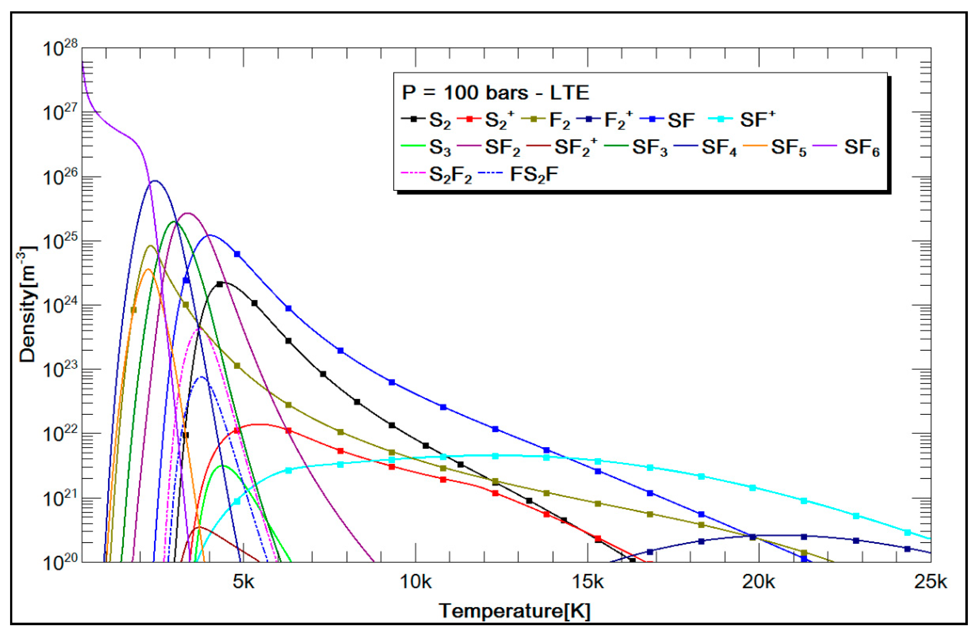
3.2.2. SF₆ and CH₄ Plasma Compositions

Using the values for σ and $\frac{\epsilon }{k_B}$ obtained from the genetic algorithm, the compositions of the SF₆ and CH₄ plasma were calculated at pressure P = 100 bar. The values proposed by the genetic algorithm to minimize the error using the same values of σ and $\frac{\epsilon }{k_B}$ for the pressure range (1 bar < P < 300 bar) and temperature (300 K < T < 60 kK) are given in

Table 8. Optimized values of σ and $\frac{\epsilon }{k_B}$ for SF₆ and CH₄, deduced from the genetic algorithm.

	σ [Å]	$\raisebox{1ex}{$\mathit{\epsilon }$}\!\left/ \!\raisebox{-1ex}{${\mathit{k}}_{\mathit{B}}$}\right.[\mathbf{K}]$
SF6	5.21279	222.27
CH4	4.083	143.57

.

The results obtained at P = 1 bar were in agreement with other authors from the literature for SF₆ [60,61,62] and CH₄ [2,4] and are not reported here. The plasma compositions at P = 100 bar using the values in Table 8 are presented in Figure 7 and Figure 8 for the case of SF₆, and in Figure 9 and Figure 10 for the case of CH₄. An increase in pressure induces changes: the higher the pressure, the higher the temperature that is needed for the dissociation of molecules. This leads to the presence of molecules at higher temperatures. The same trend is observed for ionized particles.

4. Conclusions

Software using the mass action law for obtaining the plasma composition was developed. Under the assumption of LTE, a variation of species densities with temperature can be obtained for atmospheric pressures of up to 300 bar. For such high pressures, the virial corrections that are associated with classical Debye–Hückel corrections are systematically used in ours developments. After a presentation of the theory for calculating the plasma composition, the results of the software were validated with compositions reported from the literature concerning argon and air plasmas at atmospheric pressure. Additional routines were developed using Python to automatically collect the required data from the NIST and JANAF Internet databases. To consider the high pressures, potential interactions that are formally used in virial correction were studied. We focused on the (12-6) Lennard–Jones potential, which is very commonly used in the literature. For this kind of potential, two parameters are necessary: σ, which corresponds to the distance where the potential is zero, and energy ε, corresponding to the depth of the potential. A different set of values can be found in the literature, or determined from measurements of gas mass density or viscosity. Some authors have also directly given values for the second and third virial coefficients. Nevertheless, a wide disparity appears in these two coefficients, leading to quite large differences in composition and hence mass density. Most of the time, the data given in the literature are only valid for a given pressure value, but they are not optimized for other values. We then developed a computing code based on a genetic algorithm to optimize these parameter values from the experimental data over a wide range of pressures. If no measurements are available, we suggest the use of the Stiel formulation, based on the critical values for temperature and pressure. Indeed, for temperatures and pressures that are not too close to the critical values, this formulation leads to a good compromise for values of σ and ε. The software was applied to obtain results for SF₆ and CH₄ plasma compositions at a pressure P = 100 bar.

References

1. White, W.B.; Johnson, S.M.; Dantzig, G.B. Chemical Equilibrium in Complex Mixtures. J. Chem. Phys. 1958, 28, 751–755. [Google Scholar] [CrossRef]
2. Godin, D. Calcul de Compositions Chimiques de Plasmas à l’Equilibre Thermodynamique: Application à la Modélisation de l’Ablation dans les Disjoncteurs. Master’s Thesis, Université de Montréal—Ecole Polytechnique de Montréal, Montreal, QC, Canada, 1998; 239p. [Google Scholar]
3. Godin, D.; Trépanier, J.Y. A Robust and Efficient Method for the Computation of Equilibrium Composition in Gaseous Mixtures. Plasma Chem. Plasma Process. 2004, 24, 447–473. [Google Scholar] [CrossRef]
4. Ailas, S. Etude du Spectre Moléculaire Emis par un Plasma Thermique Formé de Mélange CH4-H2. Ph.D. Thesis, Université Abou-Bekr Belkaid, Tlemcen, Algerie, 2017. [Google Scholar]
5. André, P. Etude de la Composition et des Propriétés Thermodynamiques des Plasmas Thermiques à l’Equilibre et Hors d’Equilibre Thermodynamique. Ph.D. Thesis, Université Blaise Pascal, Clermont-Ferrand, France, 1995; 123p. [Google Scholar]
6. André, P.; Brunet, L.; Duffour, E.; Lombard, J.M. Composition, Pressure and Thermodynamic Properties Calculated in Plasma Formed in Insulator Vapours of PC and POM at fixed volume. Eur. Phys. J. Appl. Phys. 2002, 17, 53–64. [Google Scholar] [CrossRef]
7. Aubreton, J. Etude des Propriétés Thermodynamiques et de Transport Dans les Plasmas à l’Equilibre et hors Equilibre Thermodynamique Appliquées aux Plasmas de Mélanges Ar-H2 et Ar-O2. Ph.D. Thesis, Université de Limoges, Limoges, France, 1985. [Google Scholar]
8. Aubreton, A. Modélisation et Etude Expérimentale d’un Plasma Métallique Crée par Ablation Laser. Ph.D. Thesis, Université de Toulouse III, Paul Sabatier, Toulouse, France, 2002; 185p. [Google Scholar]
9. Billoux, T. Elaboration d’une Base de Données Radiatives pour des Plasmas de Type CwHxOyNz et Application au Transfert Radiatif pour des Mélanges Air, CO2 et CO-H2. Ph.D. Thesis, Université de Toulouse III, Paul Sabatier, Toulouse, 2013; 180p. [Google Scholar]
10. Cabrera, A.M. Modélisation de la Cinétique Chimique d’un Plasma en Extinction dans un Disjoncteur Basse Tension. Ph.D. Thesis, Université de Toulouse III, Paul Sabatier, Toulouse, France, 2003; 177p. [Google Scholar]
11. Colombo, V.; Ghedini, E.; Sanibondi, P. Thermodynamic and Transport Properties in Non-Equilibrium Argon, Oxygen and Nitrogen Thermal Plasmas. Prog. Nuclear Energy 2008, 50, 921–933. [Google Scholar] [CrossRef]
12. Colombo, V.; Ghedini, E.; Sanibondi, P. Two Temperature Thermodynamic and Transport Properties of Argon-Hydrogen and Nitrogen-Hydrogen plasma. J. Phys. D Appl. Phys. 2009, 42, 12. [Google Scholar] [CrossRef]
13. Cressault, Y. Propriétés des Plasmas Thermiques dans des Mélanges Argon-Hydrogène-Cuivre. Ph.D. Thesis, Université de Toulouse III, Paul Sabatier, Toulouse, France, 2001; 167p. [Google Scholar]
14. Cressault, Y.; Connord, V.; Hingana, H.; Teulet, P.; Gleizes, A. Transport properties of CF3I thermal plasmas mixed with CO2, air or N2 as an alternative to SF6 plasmas in high-voltage circuit breakers. J. Phys. D Appl. Phys. 2011, 44, 495202. [Google Scholar] [CrossRef]
15. Hingana, H. Contribution à l’Etude des Propriétés des Plasmas à Deux Températures: Application A L’argon Et Air. Ph.D. Thesis, Université Toulouse III, Paul Sabatier, Toulouse, France, 2010; 143p. [Google Scholar]
16. Rat, V.; André, P.; Aubreton, J.; Elchinger, M.F.; Fauchais, P.; Vacher, D. Transport coefficients including diffusion in a two-temperature argon plasma. J. Phys. D Appl. Phys. 2002, 35, 981–991. [Google Scholar] [CrossRef]
17. Rochette, D.; Bussière, W.; André, P. Composition, Enthalpy, and Vaporization temperature, calculation of Ag-SiO2 plasmas with Air in the temperature range from 1000 to 6000 K and for pressure included between 1 and 50 bars. Plasma Chem. Plasma Process. 2004, 24, 475–492. [Google Scholar] [CrossRef]
18. Hirschfelder, J.O.; Curtiss, C.F.; Bird, R.B. Molecular Theory of Gases and Liquids; J. Wiley and Sons Chapman and Hal, Inc.: New York, NY, USA, 1954. [Google Scholar]
19. Funke, M.; Kleinrahm, R.; Wagner, W. Measurement and correlation of the (p, ρ, T) relation of sulphur hexafluoride. I. The homogeneous gas and liquid region in the temperature range from 225 K to 340 K at pressures up to 12 MPa. J. Chem. Thermodyn. 2002, 34, 717–734. [Google Scholar] [CrossRef]
20. Gilgen, R.; Kleinrahm, R.; Wagner, W. Supplementary measurements of the (pressure, density, temperature) relation of carbon dioxide in the homogeneous region at temperatures from 220 K to 360 K and pressures up to 13 MPa. J. Chem. Thermodyn. 1992, 24, 1243–1250. [Google Scholar] [CrossRef]
21. Hurly, J.J.; Defibaugh, D.R.; Moldover, M.R. Thermodynamic properties of sulfur hexafluoride. Int. J. Thermophys. 2000, 21, 739–765. [Google Scholar] [CrossRef]
22. Zarkova, L.; Hohm, U. pVT—Second virial coefficients B(T), viscosity η(T), and self-diffusion ρD(T) of the gases: BF3, CF4, SiF4, CCl4, SiCl4, SF6, MoF6, WF6, UF6, C(CH3)4, and SI(CH3)4, determined by means of an isotopic temperature-dependent potential. J. Phys. Chem. Ref. Data 2002, 31, 183–216. [Google Scholar] [CrossRef]
23. Sengers, J.M.H.L.; Klein, M.; Gallagher, J.S. Pressure-Volume-Temperature relationships of gases virial coefficients. In American Institute of Physics Handbook, 3rd ed.; McGraw-Hill: New York, NY, USA, 1971. [Google Scholar]
24. Wagner, W.; Ewers, J.; Schmidt, R. An equation of state for oxygen vapour—Second and third virial coefficients. Cryogenics 1984, 24, 37–43. [Google Scholar] [CrossRef]
25. Zarkova, L.; Hohm, U.; Damyanova, M. Viscosity and pVT-Second virial coefficient of binary noble-globular gas and globular-globular gas mixtures, calculated by means of an isotropic temperature-dependent potential. J. Phys. Chem. Ref. Data 2003, 32, 1591–1705. [Google Scholar] [CrossRef]
26. Zarkova, L.; Hohm, U.; Damyanova, M. Viscosity and pVT-Second virial coefficient, and diffusion of pure and mixed small alkanes CH4, C2H6, C3H8, n-C4H10, i-C4H10, n-C5H12, i-C5H12, and C(CH3)4, calculated by means of an isotopic temperature-dependent potential. I. Pure alkanes. J. Phys. Chem. Ref. Data 2006, 35, 1331–1364. [Google Scholar] [CrossRef]
27. Petchanka, A.; Reichert, F.; Gonzalez, J.J.; Freton, P. Modelling of deformation of PTFE nozzles in high voltage circuit breaker due to multiple interruptions. J. Phys. D Appl. Phys. 2016, 49, 135201. [Google Scholar] [CrossRef]
28. Reichert, F.; Petchanka, A.; Freton, P.; Gonzalez, J.J. Studies on the Thermal Re-ignition in SF6 High-Voltage Circuit-Breakers by means of Coupled Simulation. Plasma Phys. Technol. J. 2015, 2, 2336–2626. [Google Scholar]
29. Gonzalez, J.J.; Freton, P.; Reichert, P.; Pechanka, A. PTFE vapor contribution to pressure changes in high voltage circuit breakers. IEEE Trans. Plasma Sci. 2015, 43, 2703–2714. [Google Scholar] [CrossRef]
30. Laforest, Z.; Gonzalez, J.J.; Freton, P. Experimental study of a plasma bubble created by a wire explosion in water. Int. J. Res. Rev. Appl. Sci. 2018, 34, 93–105. [Google Scholar]
31. Benmouffok, M.; Freton, P.; Gonzalez, J.J. Theoretical plasma characterization during current pulse. Int. J. Res. Rev. Appl. Sci. 2018, 34, 3. [Google Scholar]
32. André, P.; Brunet, L.; Bussière, W.; Caillard, J.; Lombard, J.M.; Picard, J.P. Transport coefficients of plasmas consisting of insulator vapours: Application to PE, POM, PMMA, PA66 and PC. Eur. Phys. J. Appl. Phys. 2004, 25, 169–182. [Google Scholar] [CrossRef]
33. Chervy, B.; Gleizes, A.; Razafinimanana, M. Thermodynamic properties and transport coefficients in SF6-Cu mixtures at temperatures of 300 K–30 kK and pressures of 0.1–1 MPa. J. Phys. D Appl. Phys. 1994, 27, 1193–1206. [Google Scholar] [CrossRef]
34. Kravchik, T.; Sher, E.; Heywood, J.B. From spark ignition to flame initiation. Combust. Sci. Technol. 1995, 108, 1–30. [Google Scholar] [CrossRef]
35. Maly, R.; Vogel, M. Initiation and Propagation of Flame Fronts in Lean Methane/Air Mixtures by the Three Modes of the Ignition Spark. In Symposium (International) on Combustion; Elsevier: New York, NY, USA, 1979; Volume 17, pp. 821–831. [Google Scholar]
36. Zaepffel, C. Etude Expérimentale et Numérique d’une Décharge Electrique Appliquée à L’allumage d’un Milieu Réactif, Ph.D. Thesis, Université d’Orléans, Orléans, France, 2008. [Google Scholar]
37. Chase, M.W.; Davies, C.A.; Downey, J.R.; Frurip, D.J.; McDonald, R.A.; Syverud, A.N. NIST-JANAF Thermochemical Tables (ver. 1.0), Online, Standard Reference Data Program; National Institute of Standards and Technology: Gaithersburg, MD, USA, 1985. Available online: https://janaf.nist.gov/ (accessed on 7 November 2018). [CrossRef]
38. Kramida, A.; Ralchenko, Y.; Reader, J.; NIST ASD Team. NIST Atomic Spectra Database (ver. 5.5.6); Online; National Institute of Standards and Technology: Gaithersburg, MD, USA, 2018. Available online: https://physics.nist.gov/PhysRefData/ASD/levels_form.html (accessed on 7 November 2018).
39. Drawin, H.W.; Felenbok, P. Data of Plasmas in Local Thermodynamic Equilibrum; Editions Gauthier: Paris, France, 1965. [Google Scholar]
40. Hryniewicki, M.K. Accurate and Efficient Evaluation of the Second Virial Coefficient Using Practical Intermolecular Potentials for Gases. Ph.D. Thesis, University of Toronto, Toronto, ON, Canada, 2011. [Google Scholar]
41. Mamedov, B.A.; Somuncu, E. Analytical evaluation of third virial coefficient with Lennard-Jones (12-6) potential and its applications. In AIP Conference Proceedings; AIP Publishing: Melville, NY, USA, 2016; pp. 020121-1–020121-4. [Google Scholar] [CrossRef]
42. Rice, W.E.; Hirschfelder, J.O. Second virial coefficients of gases obeying a modified Buckingham (exp-6) potential. J. Chem. Phys. 1954, 22, 187–192. [Google Scholar] [CrossRef]
43. Edalat, M.; Lan, S.S.; Pang, F.; Mansoori, G.A. Optimized parameters and exponents of Mie (n, m) intermolecular potential energy function based on the shape of molecules. Int. J. Thermophys. 1980, 1, 177–184. [Google Scholar] [CrossRef]
44. Mahfouf, A. Calcul des Coefficients de Transport Dans des Plasmas Hors de L’équilibre. Ph.D. Thesis, Université Blaise Pascal, Clermont-Ferrand, France, 2016; 179p. [Google Scholar]
45. Mouritz, F.M.; Rummens, F.H.A. A critical evaluation of Lennard-Jones and Stockmayer potential parameters and of some correlation methods. Can. J. Chem. 1977, 55, 3007–3020. [Google Scholar] [CrossRef]
46. Youssef, A.; Hanna, M.M.; Saad, S.M. Determination of the Lennard-Jones force constants from diffusion measurements. Z. Phys. Chem. 1969, 241, 81–100. [Google Scholar] [CrossRef]
47. Aziz, R.A.; Slaman, M.J. An improved intermolecular potential for sulfur hexafluoride. J. Chem. Phys. 1991, 94, 2. [Google Scholar] [CrossRef]
48. Bird, R.B.; Stewart, W.E.; Lightfoot, E.N. Transport Phenomena, 2nd ed.; J. Wiley and Sons, Inc.: New York, NY, USA, 2002; ISBN 0-471-41077-5. [Google Scholar]
49. Flynn, L.W.; Thodos, G. Lennard-Jones force constants from viscosity data: Their relationship to critical properties. AIChE J. 1962, 8, 362–365. [Google Scholar] [CrossRef]
50. Hirschfelder, J.O.; Bird, R.B.; Spotz, E.L. The transport properties of gases and gaseous mixtures II. Chem. Rev. 1949, 44, 1205–1231. [Google Scholar] [CrossRef]
51. Stiel, L.I.; Thodos, G. Lennard-Jones force constants predicted from critical properties. J. Chem. Eng. Data 1962, 7, 234–236. [Google Scholar] [CrossRef]
52. Angus, S.; Armstrong, B.; Gosman, A.L.; McCarty, R.D.; Hust, J.G.; Vasserman, A.A.; Rabinovich, V.A. International Thermodynamic Tables of the Fluid State—1 Argon; Butterworths: London, UK, 1972. [Google Scholar]
53. Angus, S.; de Reuck, K.M.; Armstrong, B.; Jacobsen, R.T.; Stewart, R.B. International Thermodynamic Tables of the Fluid State—6 Nitrogen; Pergamon Press: Pergamon, NY, USA, 1979.
54. NIST Chemistry WebBook, NIST Standard Reference Database 69. Available online: https://webbook.nist.gov/chemistry/ (accessed on 7 November 2018).
55. Makarevich, L.A.; Sokolova, E.S.; Sorina, G.A. Critical parameters of Sulfur Hexafluoride. Zh Fiz. Khim. 1968, 42, 3–22. [Google Scholar]
56. Suehiro, Y.; Nakajima, M.; Yamada, K.; Uematsu, M. Critical parameters of {xCO2 + (1 − x)CHF3} for x = (1.0000, 0.7496, 0.5013, and 0.2522). J. Chem. Therm. 1996, 28, 1153–1164. [Google Scholar] [CrossRef]
57. Claus, P.; Kleinrahm, R.; Wagner, W. Measurements of the (p, ρ, T) Relation of Ethylene, Ethane, and Sulphur Hexafluoride in the Temperature Range From 235 K to 520 K at Pressures Up to 30 MPa using an Accurate Single-Sinker Densimeter. J. Chem. Thermodyn. 2003, 35, 159–175. [Google Scholar] [CrossRef]
58. Cristancho, D.E.; Mantilla, I.D.; Ejaz, S.; Hall, K.R. Accurate PρT data for methane from 300 to 450 K up to 180 MPa. J. Chem. Eng. 2010, 55, 826–829. [Google Scholar]
59. Balester, P.J.; Carter, J.N. Real-parameter Genetic Algorithms for finding Multiple Optimal Solutions in Multi-modal Optimization. In Proceedings of the Genetic and Evolutionary Computation Conference GECCO 2003, Chicago, IL, USA, 12–16 July 2003; Lecture Notes in Computer Science. Springer: Berlin/Heidelberg, Germany, 2003; Volume 2723. [Google Scholar]
60. Chervy, B. Calcul des Propriétés de Transport et Etude du Pouvoir de Coupure des Mélanges Hexafluorure de Soufre (SF6)-Fluorure de Carbone (CF4 ou C2F6) et Hexafluorure de Soufre—Vapeurs de Cuivre. Ph.D. Thesis, Université Toulouse III, Paul Sabatier, Toulouse, France, 1995; 165p. [Google Scholar]
61. Belhaouari, J.B. Modélisation de l’Extinction d’un Arc de SF6 Hors Equilibre Thermodynamique Local. Ph.D. Thesis, Université de Toulouse III, Paul Sabatier, Toulouse, France, 1997; 180p. [Google Scholar]
62. Brand, K.P.; Kopainsky, J. Particle densities in a decaying SF6 plasma. Appl. Phys. 1978, 6, 425–432. [Google Scholar] [CrossRef]
Figure 1. Evolution of species: argon; P = 1 bar − local thermal equilibrium (LTE). Comparison of ours results with Colombo et al [11], Godin [2] and Rat et al [16].
Applsci 09 00929 g001
Figure 2. Evolution of atomic species: air: P = 1 bar − LTE. Comparison of our results with P. André [5].
Applsci 09 00929 g002
Figure 3. Evolution of molecular species: air; P = 1 bar − LTE. Comparison of our results with P. André [5].
Applsci 09 00929 g003
Figure 4. The SF6 mass density at 20 bar.
Applsci 09 00929 g004
Figure 5. The SF6 mass density at 40 bar.
Applsci 09 00929 g005
Figure 6. The SF6 mass density at 100 bar.
Applsci 09 00929 g006
Figure 7. Atomic species for SF6 plasma densities at P = 100 bar − LTE.
Applsci 09 00929 g007
Figure 8. Molecular species for SF6 plasma densities at P = 100 bar − LTE.
Applsci 09 00929 g008
Figure 9. Atomic species for CH4 plasma densities at P = 100 bar − LTE.
Applsci 09 00929 g009
Figure 10. Molecular species for CH4 plasma densities at P = 100 bar − LTE.
Applsci 09 00929 g010