Meteorological Variables’ Influence on Electric Power Generation for Photovoltaic Systems Located at Different Geographical Zones in Mexico

Abstract

In this study, the relation among different meteorological variables and the electrical power from photovoltaic systems located at different selected places in Mexico were presented. The data was collected from on-site real-time measurements from Mexico City and the State of Sonora. The statistical estimation by the gradient descent method demonstrated that solar radiation, outdoor temperature, wind speed, and daylight hour influenced the electric power generation when it was compared with the real power of each photovoltaic system. According to our results, 97.63% of the estimation results matched the real data for Sonora and 99.66% the results matched for Mexico City, achieving overall errors less than 7% and 2%, respectively. The results showed an acceptable performance since a satisfactory estimation error was achieved for the estimation of photovoltaic power with a high determination coefficient R².

1. Introduction

Renewables energies represent a potential alternative in the transition towards a low-carbon society, where photovoltaic sources play a key role; however, consumers are also investors and a project is implemented only if economic conditions are verified [1].

Solar technologies are characterized depending on the way they capture, convert, and distribute sunlight such as photovoltaic (PV) systems and their corresponding requirements for an energy storage arrangement [2,3]. Consequently, these technologies feed power to the electric grid by using solar panels as generators [4,5,6]. In addition, concentrating solar power plants (CSP) use mirrors to focus the energy from the sun to drive traditional steam turbines or engines to create electricity; solar heating and cooling (SHC) systems which collect the thermal energy from the sun use this heat to provide hot water, space heating, and cooling for residential, commercial, and industrial applications. These technologies displace the need to use electricity or natural gas [7,8,9].

A photovoltaic system is composed of several components: the solar panel and the inverter for grid-connected systems and additionally energy storage for stand-alone systems. The fabrication of the solar panel involves diverse stages. The first step is to define the type of panel, where the most known is monocrystalline or polycrystalline and where the solar cells are manufactured using wafers made of silicon [10]. Nowadays, the PV systems are widely used to generate electricity due its accessible cost [5,6,11,12]. Some studies aimed at reducing this cost even more, e.g., in Reference [13], a design optimization model for the residential PV systems in South Korea was proposed, where the objective function to be minimized consisted of three costs, such as the monthly electric bill, the PV-related construction costs, and the PV-related maintenance cost.

The solar radiation (photons) is responsible for the photovoltaic effect; nonetheless, some weather factors have an effect on the amount of energy generated even with the optimum radiation. A cloudy day generates a shadow on the solar panel by the time it has to capture the photons so that the incidence of these particles will be less, achieving a minor electric power. It is well-known that clouds are water steam concentrated in the air; in other words, humidity and temperature work together, and such a relation is an example of how the meteorological variables impact the generation of electric power [14,15].

Solar energy, besides wind energy, is currently the most resourceful renewable source worldwide [16,17]. Its obtainment, unlike many others currently used, does not mean any harm to the environment, and its resources overcome, by far, everyone else [12,18,19,20]. Some countries such as Germany, Italy, Spain, United States of America, and China are ahead on solar energy research; meanwhile in Mexico, being a country rich in solar radiation, with a great territorial extension, and having some solar energy studies, solar energy still does not have the necessary research compared to countries leading solar technology [4,5,6,11,12,21].

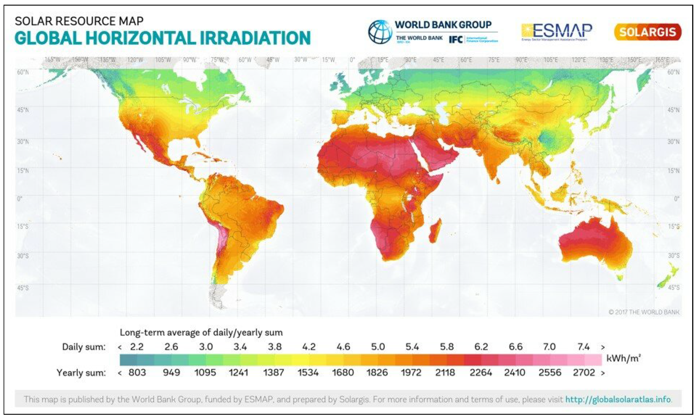
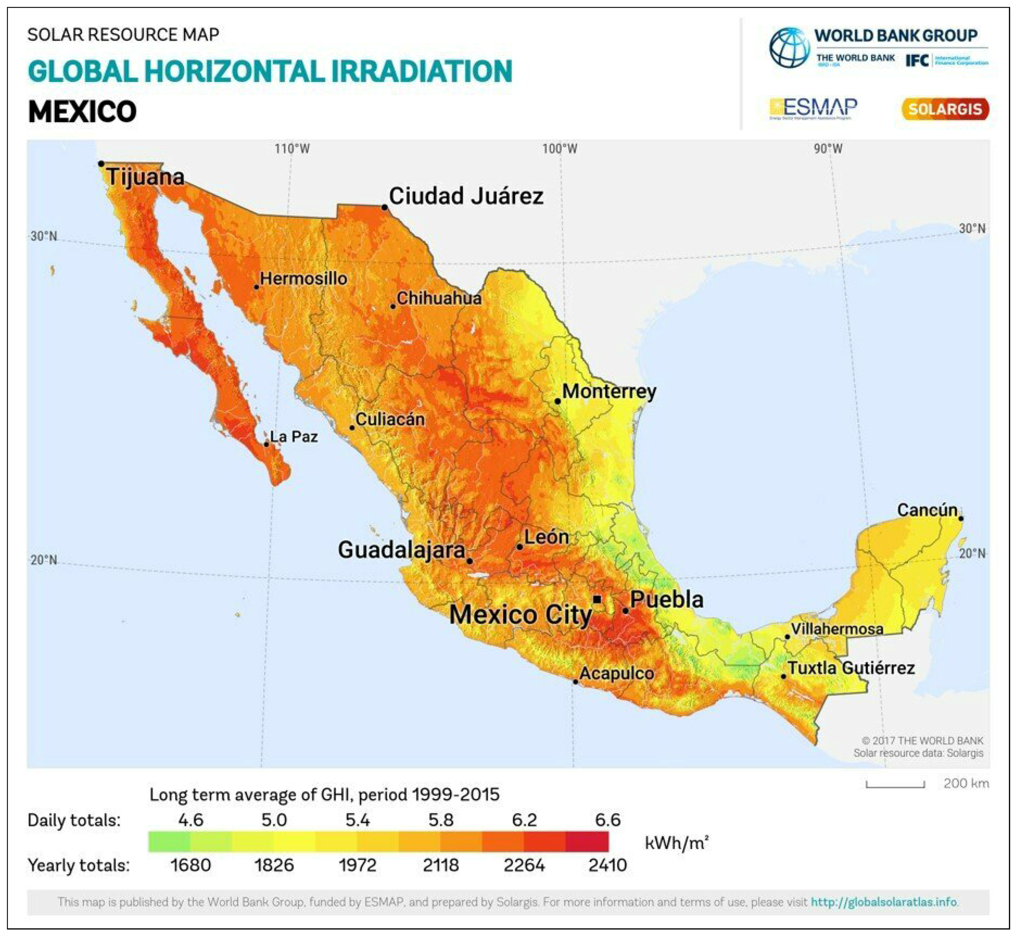
Figure 1 depicts the behavior of the horizontal solar radiation on the world. Similarly, if Mexico is compared with Europe, it can be seen that the only country with a notorious radiation incidence is Spain, achieving a maximum value between 4.8 and 5.4 kWh/m² [22]. Mexico exceeds Spain both in incidence territory and in radiation intensity, with an average between 5.6 and 6.2 kWh/m², as can be seen in Figure 2, exceeding even China, which mostly contemplates values of 4.6 kWh/m².

Table 1 shows the data compilation from 2010 describing the global-horizontal solar radiation for some locations in Mexico. The total irradiation provided by solar energy in the year 2018 was summarized in Reference [25]. Both reports agree that the Northwest of Mexico reached the maximum values, the states of Sonora, Baja California, Coahuila, and Chihuahua being the main producers/receivers.

Recently, diverse reports have studied the relations between some meteorological variables and the electric power generated in a photovoltaic system. In Reference [26], an analysis of the climatic factors and solar data from the Andes site was performed; nonetheless, all the data gathered for the study was averaged every 10 min and the power measurements were estimated. In [27], the effect of diverse meteorological variables (outdoor temperature, air pressure, humidity, wind speed, and solar radiation) on the generated energy are mentioned, although a representative model of the plant was not obtained and all the data was experimentally generated. In Reference [28], a statistical method was applied to forecast the energy generated by a solar plant, though a database of 30 plants from different locations is necessary and although it does not have real power measurements from the site and the computational load is heavy. In Reference [29], an artificial neural network (ANN) is used to obtain a model to forecast the photovoltaic energy; however, the solar radiation was the only meteorological variable analyzed.

Higher Education Institutions (HEI) currently play a major role in the generation of human capital and the associated impact on societal development; HEIs are ideal locations to focus the resources in terms of the deployment and experimentation of decarbonization technologies to demonstrate the best practice for a further replication within wider society [30].

Careful planning is required to manage the future electricity demand of PV systems due to its increasing potential demand in Mexico [31,32]. Therefore, it is vital to understand the influence of meteorological variables on energy consumption in which a better understanding of it can contribute to a more useful strategy in meeting the energy efficiency goal for the country.

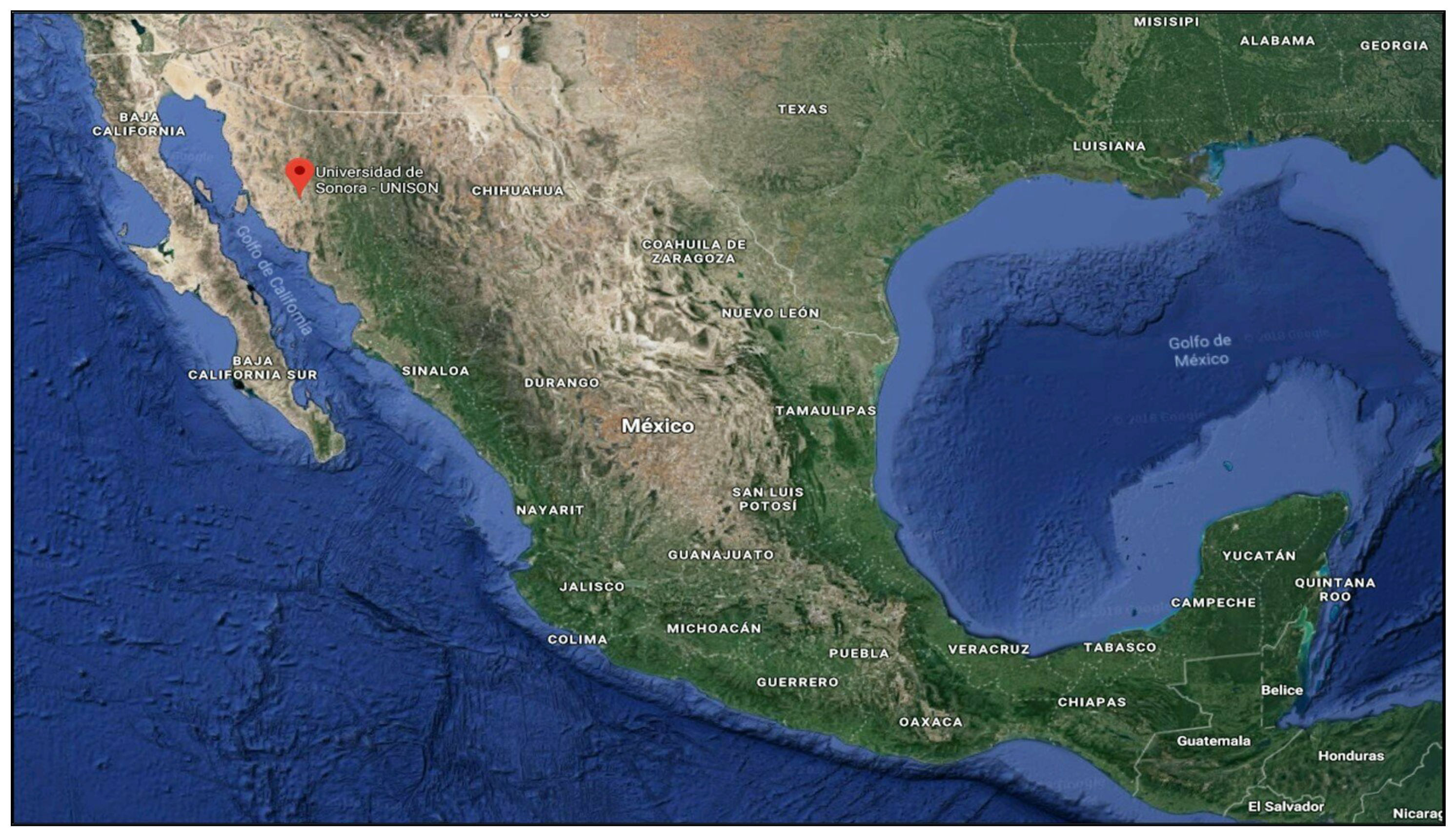
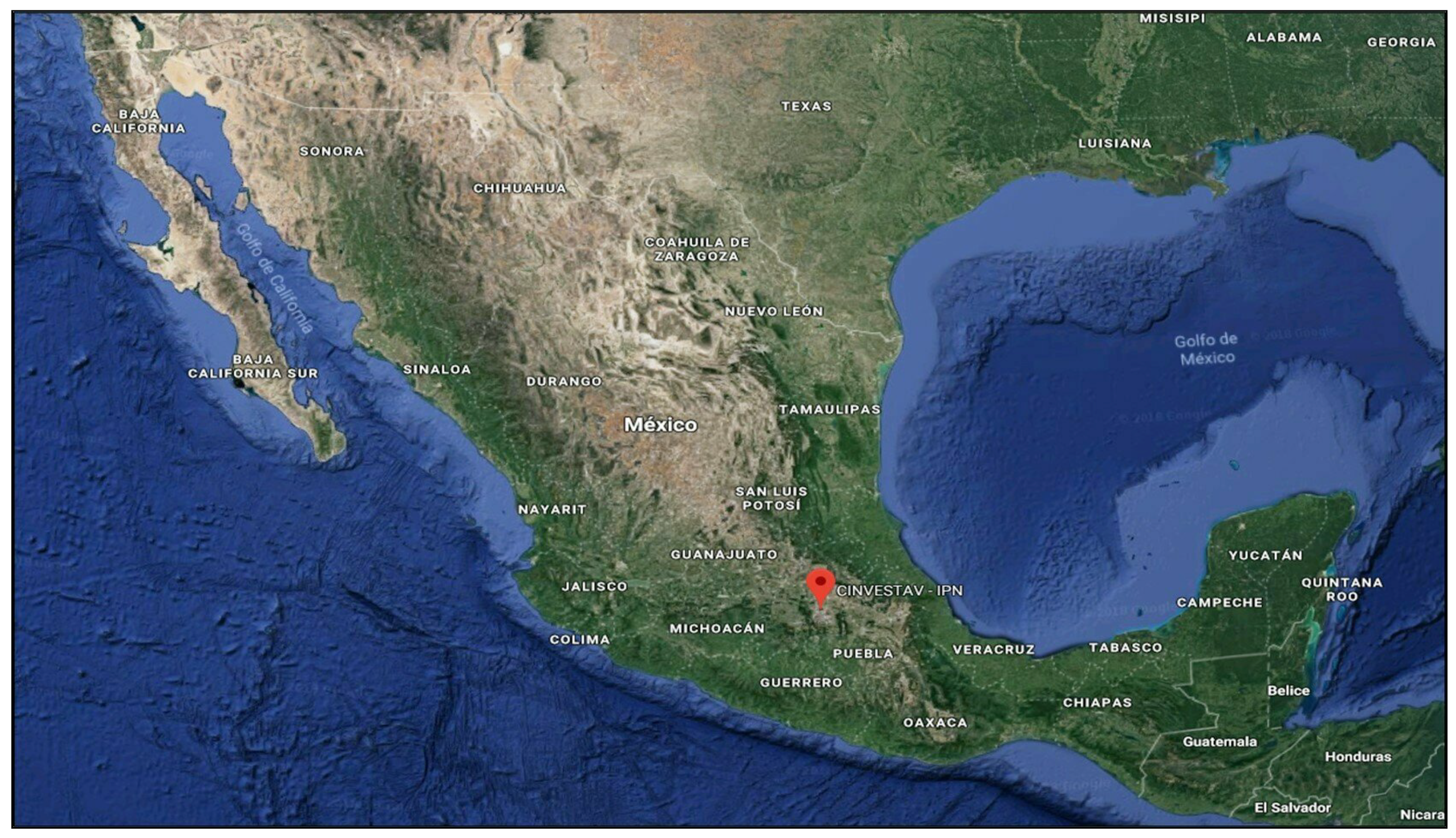
According to the above and considering References [1,13,30], the aim of this work is to present a statistical analysis based on the gradient descent method that is easy to implement and has a low computational load to estimate the electric power generation from the meteorological data such as the solar radiation, outdoor temperature, wind speed, and daylight time collected from PV systems located in Mexico City and Sonora [33]. This is important because most of the current photovoltaic system deployments do not monitor these factors or employ them in adaptation and prediction tasks [34,35,36].

The proposed methodology achieves a satisfactory estimation of the PV power with a high determination coefficient and a fair error percentage value.

Table 1. The solar radiation on select places in Mexico (data in kWh/m² per day) [37].

State	City	Jan	Feb	Mar	Apr	May	Jun	Jul	Aug	Sep	Oct	Nov	Dec	Avg
Sonora	Hermosillo	4.0	4.6	5.4	6.6	8.3	8.5	6.9	6.6	6.7	6.0	4.7	3.9	6.0
Sonora	Guaymas	4.5	5.7	6.5	7.2	7.3	6.8	5.9	5.8	6.3	5.9	5.0	5.6	5.9
Chihuahua	Chihuahua	4.1	4.9	6.0	7.4	8.2	8.1	6.8	6.2	5.7	5.2	4.6	3.8	5.9
SLP	SLP	4.3	5.3	5.8	6.4	6.3	6.1	6.4	6.0	5.5	4.7	4.2	3.7	5.4
Zacatecas	Zacatecas	4.9	5.7	6.6	7.5	7.8	6.2	6.2	5.9	5.4	4.8	4.8	4.1	5.8
Guanajuato	Guanajuato	4.4	5.1	6.1	6.3	6.6	6.0	6.0	5.9	5.8	5.2	4.8	4.6	5.6
Aguascalientes	Aguascalientes	4.5	5.2	5.9	6.6	7.2	6.3	6.1	5.9	5.7	5.1	4.8	4.0	5.6
Oaxaca	Salina Cruz	5.4	6.3	6.6	6.4	6.1	5.0	5.6	5.9	5.2	5.9	5.7	5.2	5.8
Oaxaca	Oaxaca	4.9	5.7	5.8	5.5	6.0	5.4	5.9	5.6	5.0	4.9	4.8	4.4	5.3
Jalisco	Colotlán	4.6	5.7	6.5	7.5	8.2	6.6	5.8	5.6	5.8	5.3	4.9	4.1	5.9
Jalisco	Guadalajara	4.6	5.5	6.3	7.4	7.7	5.9	5.3	5.3	5.2	4.9	4.8	4.0	5.6
Durango	Durango	4.4	5.4	6.5	7.0	7.5	6.8	6	5.6	5.7	5.1	4.8	3.9	5.7
Baja California	La Paz	4.4	5.5	6.0	6.6	6.5	6.6	6.3	6.2	5.9	5.8	4.9	4.2	5.7
Baja California	San Javier	4.2	4.6	5.3	6.2	6.5	7.1	6.4	6.3	6.4	5.1	4.7	3.7	5.5
Baja California	Mexicali	4.1	4.4	5.0	5.6	6.6	7.3	7.0	6.1	6.1	5.5	4.5	3.9	5.5
Querétaro	Querétaro	5.0	5.7	6.4	6.8	6.9	6.4	6.4	6.4	6.3	5.4	5.0	4.4	5.9
Puebla	Puebla	4.9	5.5	6.2	6.4	6.1	5.7	5.8	5.8	5.2	5.0	4.7	4.4	5.5
Hidalgo	Pachuca	4.6	5.1	5.6	6.8	6.0	5.7	5.9	5.8	5.3	4.9	4.6	4.2	5.4

Table 1. The solar radiation on select places in Mexico (data in kWh/m² per day) [37].

State	City	Jan	Feb	Mar	Apr	May	Jun	Jul	Aug	Sep	Oct	Nov	Dec	Avg
Sonora	Hermosillo	4.0	4.6	5.4	6.6	8.3	8.5	6.9	6.6	6.7	6.0	4.7	3.9	6.0
Sonora	Guaymas	4.5	5.7	6.5	7.2	7.3	6.8	5.9	5.8	6.3	5.9	5.0	5.6	5.9
Chihuahua	Chihuahua	4.1	4.9	6.0	7.4	8.2	8.1	6.8	6.2	5.7	5.2	4.6	3.8	5.9
SLP	SLP	4.3	5.3	5.8	6.4	6.3	6.1	6.4	6.0	5.5	4.7	4.2	3.7	5.4
Zacatecas	Zacatecas	4.9	5.7	6.6	7.5	7.8	6.2	6.2	5.9	5.4	4.8	4.8	4.1	5.8
Guanajuato	Guanajuato	4.4	5.1	6.1	6.3	6.6	6.0	6.0	5.9	5.8	5.2	4.8	4.6	5.6
Aguascalientes	Aguascalientes	4.5	5.2	5.9	6.6	7.2	6.3	6.1	5.9	5.7	5.1	4.8	4.0	5.6
Oaxaca	Salina Cruz	5.4	6.3	6.6	6.4	6.1	5.0	5.6	5.9	5.2	5.9	5.7	5.2	5.8
Oaxaca	Oaxaca	4.9	5.7	5.8	5.5	6.0	5.4	5.9	5.6	5.0	4.9	4.8	4.4	5.3
Jalisco	Colotlán	4.6	5.7	6.5	7.5	8.2	6.6	5.8	5.6	5.8	5.3	4.9	4.1	5.9
Jalisco	Guadalajara	4.6	5.5	6.3	7.4	7.7	5.9	5.3	5.3	5.2	4.9	4.8	4.0	5.6
Durango	Durango	4.4	5.4	6.5	7.0	7.5	6.8	6	5.6	5.7	5.1	4.8	3.9	5.7
Baja California	La Paz	4.4	5.5	6.0	6.6	6.5	6.6	6.3	6.2	5.9	5.8	4.9	4.2	5.7
Baja California	San Javier	4.2	4.6	5.3	6.2	6.5	7.1	6.4	6.3	6.4	5.1	4.7	3.7	5.5
Baja California	Mexicali	4.1	4.4	5.0	5.6	6.6	7.3	7.0	6.1	6.1	5.5	4.5	3.9	5.5
Querétaro	Querétaro	5.0	5.7	6.4	6.8	6.9	6.4	6.4	6.4	6.3	5.4	5.0	4.4	5.9
Puebla	Puebla	4.9	5.5	6.2	6.4	6.1	5.7	5.8	5.8	5.2	5.0	4.7	4.4	5.5
Hidalgo	Pachuca	4.6	5.1	5.6	6.8	6.0	5.7	5.9	5.8	5.3	4.9	4.6	4.2	5.4

2. Methodology

2.1. Statistical Method

The amount of data collected and the correlation among them are quite important to accomplish an estimation. If the total data is scarce or the correlation between any input and the output is low, the estimation will not be satisfactory.

The correlation analysis is one of the most used and reported statistical methods on scientist and medical researches; its visual representation is known as a dispersion graphic. It is used to prove or reject the existence of a relation between two different variables based on the Pearson correlation coefficient described by Equation (1).

$$\rho \left(a,b\right)=\frac{E\left(ab\right)}{{\sigma }_a{\sigma }_b}$$

(1)

where $E\left(ab\right)$ is the crossed correlation between a and b and where ${\sigma }_a^2=E\left(a^2\right)$ and ${\sigma }_b^2=E\left(b^2\right)$ are the variations of the variables a and b, respectively [38].

If “a” and “b” are the two considerate variables, then a dispersion graphic shows the location of each ordered pair in a coordinated system. If most points appear to be close to a straight line, this correlation is known as linear. If most points appear to be close to a curve, the correlation is known as nonlinear. On the other hand, if a clear pattern among the ordered pairs is inexistent, then there is no relation between both variables [39]. In order to represent the curve (curve or line regression) that best fits the behavior of ordered pairs, Equation (2) is used.

$$y=a_0+a_{1}x+a_2{x}^2+a_3{x}^3+\cdots +a_m{x}^m$$

(2)

The correlation coefficient or R requires that both a magnitude and a direction be either positive (from 0 to 1) or negative (from −1 to 0). If R gets close to $\pm 1$, the correlation will be stronger. The correlation does not depend on the direction or the sign: A correlation of 0.57 is equal to a −0.57 one.

It can be also stated that the greater the absolute value of R, the greater the correlation will be. The determination coefficient $R^2$ is defined as the percentage of the variation of the dependent variable values that can be explained as variations of the independent variable. In other words, a determination coefficient $R^2$ = 0.23 symbolizes that 23% of the dependent variables is attached to the changes of the independent variable. Therefore, if a correlation factor of R = 0.20 was found between two variables, the determination coefficient would be $R^2$ = 0.04 so that only 4% of the dependent variable is affected by the variations of the independent variable [40].

In order to create a statistical representative model of the generated power by solar energy, the concept of gradient descent optimization (GDO) was considered due its ability to minimize the model error by the LSR of a linear regression model, which is often used on estimation studies, but it is not as complex to implement as an intelligent technique [29,41,42].

This optimization method has multiple applications. In Reference [43], this method was used to optimize the geometry of the strut-and-tie truss to minimize the difference in the share of resisting actions with respect to the prediction of the multi-action shear model. In Reference [44], a model based on gradient descent is proposed that integrates several important parameters for ranking channels in order to select the best communication channel from a radio spectrum for transmission, enhanced by cognitive radio as an intelligent wireless solution.

The GDO is based on the linear regression method known as the relation among all the input variables and the output one. Depending on the number of input variables, the regression can be simple or multiple [45,46,47]. To organize all the gathered data, every input variable is considered as a column in a matrix called “X” and the output parameter is considered as a vector “y”, as seen in Equation (3).

$$X=\left[\begin{array}{ccccc}{x}_{11}& x_{12}& x_{13}& \cdots & x_{1k}\\ x_{21}& x_{22}& x_{23}& \cdots & x_{2k}\\ x_{31}& x_{32}& x_{33}& \cdots & x_{3k}\\ ⋮& ⋮& ⋮& & ⋮\\ x_{n1}& x_{n2}& x_{n3}& \cdots & x_{nk}\end{array}\right]y=\left[\begin{array}{c}{y}_1\\ y_2\\ ⋮\\ y_n\end{array}\right]$$

(3)

The purpose of GDO is to find an estimation of the real output through an equation involving all the collected data as shown in Equation (4).

$$h_{\theta }\left(x\right)={\theta }_0+{\theta }_1{x}_1+{\theta }_2{x}_2+\dots +{\theta }_k{x}_k+\epsilon$$

(4)

where $h_{\theta }\left(x\right)$ is the estimated output, $x_k$ is the kth input variable, ${\theta }_k$ is the characteristic coefficient of every variable, and $ϵ$ is the error between the model and the real data [48].

As can be seen from Equation (4), ${\theta }_0$ is not a value of influence for any input; however, it does locate the resulting estimation graphic on the Y-axis. If ${\theta }_0$ is greater than expected, the plot will have a wide gap against the real data in the lower values; nonetheless, if ${\theta }_0$ is smaller than necessary, the gap between the real and estimated model will be large on the upper zone. Therefore, both cases have a greater error. In order to achieve the minimum error value and instead of a linear regression which uses the least squares method, the GDO finds the right ${\theta }_0$ by recursive partial derivatives of the cost function described by Equation (5)

$$J\left[\theta \right]=\frac{1}{2m}\sum _{i=1}^m{\left(h_{\theta }\left(x^{\left(i\right)}\right)-y^{\left(i\right)}\right)}^2$$

(5)

where m is the total amount of rows in the matrix, $x\left(i\right)$ represents the ith row of “X”, and $y\left(i\right)$ is the value of the ith row of “y”. The gradient descent, denoted by Equation (6), aims to converge to the cost function minimum through its partial derivative. The quickness of the convergence is given by $\alpha$.

$${\theta }_k:={\theta }_k-\alpha \frac{\partial }{\partial {\theta }_k}J\left[\theta \right]$$

(6)

Equation (7) shows the substitution of Equation (5) into (6) which has to be repeated itself n-times until the convergence is done.

$${\theta }_k:={\theta }_k-\alpha \frac{1}{m}\sum _{i=1}^m\left(h_{\theta }\left(x^{\left(i\right)}\right)-y^{\left(i\right)}\right)·x_k^{\left(i\right)}$$

(7)

2.2. Solar Data

The data gathered from the State of Sonora, specifically the city of Hermosillo, were obtained with the support of the University of Sonora (UNISON), while the ones from Mexico City were issued by the Centro de Investigación y de Estudios Avanzados (CINVESTAV) campus Zacatenco, with the solar radiation (global-horizontal), outside temperature, wind speed, and daylight hour (time) as the input meteorological variables and the electric power as the output for both PV systems. Considering that both the solar plants are from different locations and do not have the same arrangement, their respective output power magnitudes vary among them; Hermosillo site has an electric power maximum around 2500 W, while Mexico City site reaches values around 45 kW.

The matrix “X” and the vector “y” from Equation (3) are shown in Equation (8).

$$\begin{array}{c}X=\left[\begin{array}{cccc}Solarradiation& Temperature& Windspeed& Time\end{array}\right]\\ y=\left[ElectricPower\right]\end{array}$$

(8)

By using the same variables from both locations, the aim is to achieve an acceptable statistical estimation of the electric power even if those variables are gathered from distant geographic areas.

3. Results and Discussion

3.1. Hermosillo Site

Figure 3 shows the geographical zone where Hermosillo Site (HS) is located. This site covers a period data of 6 months. Figure 4, Figure 5, Figure 6 and Figure 7 depict the dispersion graphic and fitted curve for each input variable against the electric power. In

Table 2. The fitted curve characteristic equation of every input from HS.

Month	Input Variables
	Solar radiation	Temperature
Aug	$f\left(x\right)=2.245x+92.59$	$f\left(x\right)=-17.98x^2+1274x-\mathrm{20,920}$
Sep	$f\left(x\right)=2.308x+28.45$	$f\left(x\right)=-11.43x^2+796.7x-\mathrm{12,210}$
Oct	$f\left(x\right)=2.276x+50.32$	$f\left(x\right)=-8.751x^2+556.5x-7217$
Nov	$f\left(x\right)=2.326x-29.48$	$f\left(x\right)=-6.074x^2+354.8x-3505$
Dec	$f\left(x\right)=2.25x-36.17$	$f\left(x\right)=0.08391x^2+45.57x+219.1$
Jan	$f\left(x\right)=2.398x+8.88$	$f\left(x\right)=-2.016x^2+144.8x-752.7$
TOTAL	$f\left(x\right)=2.296x-1.747$	$f\left(x\right)=-1.751x^2+124.2x-581.9$
	Wind speed	Hour
Aug	$f\left(x\right)=-60.94x^2+438.2x+753.3$	$f\left(x\right)=-\mathrm{43,250}{x}^2+\mathrm{44,070}x-8893$
Sep	$f\left(x\right)=-21.89x^2+111.6x+1352$	$f\left(x\right)=-\mathrm{42,970}{x}^2+\mathrm{43,290}x-8593$
Oct	$f\left(x\right)=-20.63x^2+118.4x+1292$	$f\left(x\right)=-\mathrm{46,940}{x}^2+\mathrm{46,740}x-9314$
Nov	$f\left(x\right)=4.208x^2+12.31x+1348$	$f\left(x\right)=-\mathrm{50,610}{x}^2+\mathrm{50,160}x-\mathrm{10,180}$
Dec	$f\left(x\right)=-11.68x^2+120.2x+1005$	$f\left(x\right)=-\mathrm{51,600}{x}^2+\mathrm{51,860}x-\mathrm{10,900}$
Jan	$f\left(x\right)=-14.18x^2+206.8x+886.7$	$f\left(x\right)=-\mathrm{55,500}{x}^2+\mathrm{56,360}x-\mathrm{11,960}$
TOTAL	$f\left(x\right)=-14.47x^2+138.7x+1096$	$f\left(x\right)=-\mathrm{49,950}{x}^2+\mathrm{50,110}x-\mathrm{10,360}$

and

Table 3. The determination coefficients (R²) of every input from HS.

Month	Solar Radiation	Temperature	Wind Speed	Hour
Aug	0.9917	0.1679	0.0541	0.9825
Sep	0.9981	0.1502	0.0242	0.9968
Oct	0.9523	0.1664	0.0380	0.9850
Nov	0.9708	0.1955	0.0135	0.9962
Dec	0.9851	0.0965	0.0136	0.8865
Jan	0.9609	0.1390	0.0565	0.9760
TOTAL	0.9532	0.1077	0.0140	0.8098

, the monthly and total results of the characteristic equations for each fitted curve and their determination coefficients are described, respectively.

Equation (7) is applied in order to calculate the values of ${\theta }_k$ for Hermosillo by using the Matlab^® software. The optimal values found for $\theta$ are mentioned in

Table 4. The values of ${\theta }_k$ from HS by gradient descent.

${\mathit{\theta }}_{\mathit{k}}$	HS
${\theta }_0$	0.0044
${\theta }_1$	2.2387
${\theta }_2$	0.1156
${\theta }_3$	0.0154
${\theta }_4$	0.0022

and substituted into Equation (4), thereby obtaining its mathematical representation given by Equation (9). Figure 8 is obtained by implementing six months of gathered data into Equation (9). It describes the behavior of the statistical estimation (red) against the real data (green) obtained by the PV system in Hermosillo. For a better appreciation of these results, Figure 9 shows a close-up from 24 November to 24 December 2018. A tracing practically coincident with the rise and fall times for each day as a satisfactory reach of the maximum and minimum values is observed.

$$h_{\theta }=0.0044+2.2387x_1+0.1156x_2+0.0154x_3+0.0022x_4$$

(9)

3.2. Data from Mexico City

The geographical zone of the Mexico City Site (MCS) is presented in Figure 10. The data covers a period of 6 months. From Figure 11, Figure 12, Figure 13 and Figure 14 the dispersion graphic and fitted curve for each input variable against electric power are shown. In

Table 5. The fitted curve characteristic equation of every input from MCS.

Month	Input Variables
	Solar radiation	Temperature
Jul	$f\left(x\right)=53.58x+135$	$f\left(x\right)=-20.07x^2+3392x-\mathrm{44,530}$
Aug	$f\left(x\right)=56.62x+241.2$	$f\left(x\right)=-43.78x^2+4162x-\mathrm{51,030}$
Sep	$f\left(x\right)=59.48x+245.7$	$f\left(x\right)=9.184x^2+1875x-\mathrm{25,960}$
Oct	$f\left(x\right)=57.58x+189.8$	$f\left(x\right)=-6.143x^2+2115x-\mathrm{18,990}$
Nov	$f\left(x\right)=57.64x+1.454$	$f\left(x\right)=-132x^2+5978x-\mathrm{36,790}$
Dec	$f\left(x\right)=53.52x-7.362$	$f\left(x\right)=-104.9x^2+4312x-\mathrm{18,320}$
TOTAL	$f\left(x\right)=56.75x+65.85$	$f\left(x\right)=31.9x^2+203.1x+2471$
	Wind speed	Hour
Jul	$f\left(x\right)=-173.8x^2+531.6x+\mathrm{20,420}$	$f\left(x\right)=-\mathrm{584,100}{x}^2+\mathrm{632,300}x-\mathrm{137,600}$
Aug	$f\left(x\right)=-157.7x^2+325.2x+\mathrm{21,850}$	$f\left(x\right)=-\mathrm{599,500}{x}^2+\mathrm{649,400}x-\mathrm{141,400}$
Sep	$f\left(x\right)=-156.4x^2+459.8x+\mathrm{19,960}$	$f\left(x\right)=-\mathrm{632,500}{x}^2+\mathrm{686,200}x-\mathrm{153,700}$
Oct	$f\left(x\right)=-113x^2+47.06x+\mathrm{23,490}$	$f\left(x\right)=-\mathrm{693,400}{x}^2+\mathrm{735,600}x-\mathrm{159,300}$
Nov	$f\left(x\right)=66.96x^2-1894x+\mathrm{28,680}$	$f\left(x\right)=-\mathrm{918,400}{x}^2+\mathrm{908,400}x-\mathrm{181,500}$
Dec	$f\left(x\right)=44.08x^2-706.9x+\mathrm{22,910}$	$f\left(x\right)=-\mathrm{837,800}{x}^2+\mathrm{843,100}x-\mathrm{175,100}$
TOTAL	$f\left(x\right)=-130.7x^2+61.23x+\mathrm{22,720}$	$f\left(x\right)=-\mathrm{617,100}{x}^2+\mathrm{650,100}x+\mathrm{136,600}$

and

Table 6. The determination coefficients (R²) of every input from MCS.

Month	Solar Radiation	Temperature	Wind Speed	Hour
Jul	0.9997	0.4952	0.0295	0.6032
Aug	0.9990	0.3261	0.0214	0.5652
Sep	0.9950	0.3684	0.0093	0.5014
Oct	0.9923	0.2148	0.0177	0.5803
Nov	0.9995	0.1674	0.0320	0.8684
Dec	0.9995	0.1440	0.0015	0.8865
TOTAL	0.9989	0.2052	0.0178	0.5725

, the monthly and total results of the characteristic equations for each fitted curve and their determination coefficients are described, respectively.

The determination coefficient values for Mexico City are found applying the same procedure used in the case of Hermosillo, as shown in Table 6. Analogous to the case from Hermosillo, the coefficients $\theta$ for Mexico City data and its mathematical representation are displayed in

Table 7. The values of ${\theta }_k$ from MCS by gradient descent.

${\mathit{\theta }}_{\mathit{k}}$	MCS
${\theta }_0$	0.1005
${\theta }_1$	55.9815
${\theta }_2$	2.2910
${\theta }_3$	0.1290
${\theta }_4$	0.0533

and Equation (10), respectively. Figure 15 shows a six months estimation result (red) against the real data behavior (green) from Mexico City. In order to a better appreciation, Figure 16 shows a close-up of Figure 15 covering the same period as that in the case of Hermosillo. The estimation result matches with the rise and fall times of the real power.

$$h_{\theta }=0.1005+55.9815x_1+2.2910x_2+0.1290x_3+0.0533x_4$$

(10)

3.3. Error Analysis On-Site

As seen in Section 1 and according to Reference [51], the output power of a PV array greatly depends, among other parameters, on solar radiation; however, this variable has an intermittent nature and suffers from rapid fluctuations. In Reference [41,51], the above is considered and some parameters besides the solar radiation such as clear sky or weather data are added; nonetheless, for these cases, the solar radiation is either the estimated output or an estimated input, contrary to this paper where this variable is measured on-site.

Each coefficient ${\theta }_k$ from Equations (9) and (10) represents the characteristic magnitude of its respective input variable $x_k$. Its quantity values prove the influence in the mathematical model approximation, establishing an existing relationship between the meteorological variables involved and (responsible for solar fluctuations) the power output.

Comparing Figure 9 and Figure 16, an adequate behavior is observed between both results, achieving a valid statistical estimation. Regardless of the amount of stored data, similar outcomes were obtained from both locations.

This statement is mathematically proved through the correlation and error analysis.

3.3.1. Correlation Analysis

According to Section 2.1, the smaller an error between the estimation and real data, the greater the determination coefficient will be. Figure 17 and Figure 18 show the dispersion graphic of the estimation against the real electric power for Hermosillo and Mexico City respectively. Moreover, in

Table 8. The monthly and total fitted curve characteristic equation and determination coefficient values of estimation for both locations.

Location	Month	Fitted Curve	R2
	Aug	$f\left(x\right)=1.005x+84.92$	0.9916
	Sep	$f\left(x\right)=1.032x+20.92$	0.9981
	Oct	$f\left(x\right)=1.031x+44.45$	0.9877
HS	Nov	$f\left(x\right)=1.022x-29.74$	0.9926
	Dec	$f\left(x\right)=1.05x-37.57$	0.9849
	Jan	$f\left(x\right)=1.009x+6.707$	0.9982
	TOTAL	$f\left(x\right)=1.025x-4.633$	0.9763
	Jul	$f\left(x\right)=1.003x+91.51$	0.9989
	Aug	$f\left(x\right)=1.01x+184.3$	0.9961
	Sep	$f\left(x\right)=0.9843x+525.7$	0.9946
MCS	Oct	$f\left(x\right)=1.003x+140.6$	0.9997
	Nov	$f\left(x\right)=1.007x-40.05$	0.9982
	Dec	$f\left(x\right)=1.004x-44.28$	0.9995
	TOTAL	$f\left(x\right)=1.014x+19.18$	0.9966

, the monthly and total fitted curve characteristic equation and determination coefficients for both cases are displayed.

Both statistical models estimate favorably the real electric power for each tested day as we can observe through the values in Table 8. A great closeness can be confirmed between the estimation and the real data for each location, which shows that the implementation of a gradient descent optimization achieves a satisfactory result.

3.3.2. Error Analysis

The less the difference between the estimated and the real value, the better the estimation. Two kinds of errors were applied, where “$P_m$” was the measured power, “$P_e$” was the estimated power, “s” was the sample in consideration, and “N” was the total amount of samples. The first one was called Mean Absolute Error (MAE) defined by Equation (11) and was used as a standard statistical metric to measure the model performance in meteorology, air quality, and climate research studies [42,51,52]. The second one was the percentage of the MAE known as Mean Absolute Percentage Error (MAPE) defined by Equation (12).

Given that the results shown in Figure 9 and Figure 16 resemble a sinusoidal behavior, $\left(P_m-P_e\right)/P_m$ does not present the real error between both signals. Considering Figure 19a, if the measured value is on a high level, then the rate between the $P_m-P_e$ and $P_m$ values will be low; however, if the measured value is on a low level, then the same rate will be high or close to 1, as seen in Figure 19b. According to this, the rate is changed regarding the full range of the measured signal (max-min) instead in order to obtain a reliable value. Equation (13) represents the modified MAPE.

$$MAE=\frac{{\displaystyle \sum _{s=1}^N}\left|P_m-P_e\right|}{N}$$

(11)

$$MAP{E}_{\%}=\frac{{\displaystyle \sum _{s=1}^N}\left|\frac{P_m-P_e}{P_m}\right|}{N}·100$$

(12)

$$MAP{E_{\left(range\right)}}_{\%}=\frac{{\displaystyle \sum _{s=1}^N}\left|\frac{P_m-P_e}{max\left(P_m\right)-min\left(P_m\right)}\right|}{N}·100$$

(13)

With respect to the data from HS and MCS,

Table 9. The error values between the estimated and real data.

Location	Month	MAE	MAPE (Range)
	Aug	299.7928 W	11.9436%
	Sep	203.7386 W	7.5643%
	Oct	267.9841 W	9.2382%
HS	Nov	138.1913 W	5.1418%
	Dec	178.9316 W	7.0381%
	Jan	184.5001 W	6.7978%
	TOTAL	200.0924 W	6.8859%
	Jul	590.6460 W	1.0480%
	Aug	1192.3 W	2.0392%
	Sep	726.2990 W	1.2646%
MCS	Oct	741.8355 W	1.2660%
	Nov	741.4300 W	1.3534%
	Dec	812.8113 W	1.7237%
	TOTAL	1130.4 W	1.9291%

shows the values of the errors mentioned in Equations (11) and (13).

Table 9 shows the errors for both locations, where the MAE result values for HS have a range from 138.1913 W to 299.7928 W and an overall of 200.6071 W. Considering MCS, its MAE goes from 590.6460 W to 1192.3 W, with an overall of 1130.4 W. From these results we can highlight that the values are low according to the total value range for each location, being up to 2500 W and 45 kW for HS and MCS, respectively. This statement is proven by column 4 from Table 9, achieving a MAPE of 6.9036% in general for HS; meanwhile, for MCS, its respective results is a MAPE of 1.9291%. The above demonstrates the estimation robustness of the statistical model.

4. Conclusions

A gradient descent method was used to calculate, through a characteristic equation, the relationship between several variables which can be easily computed using quantitative data.

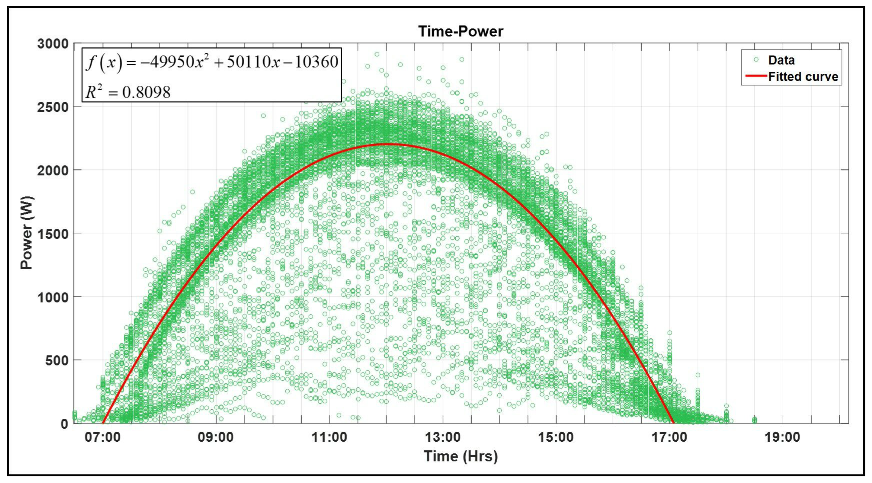
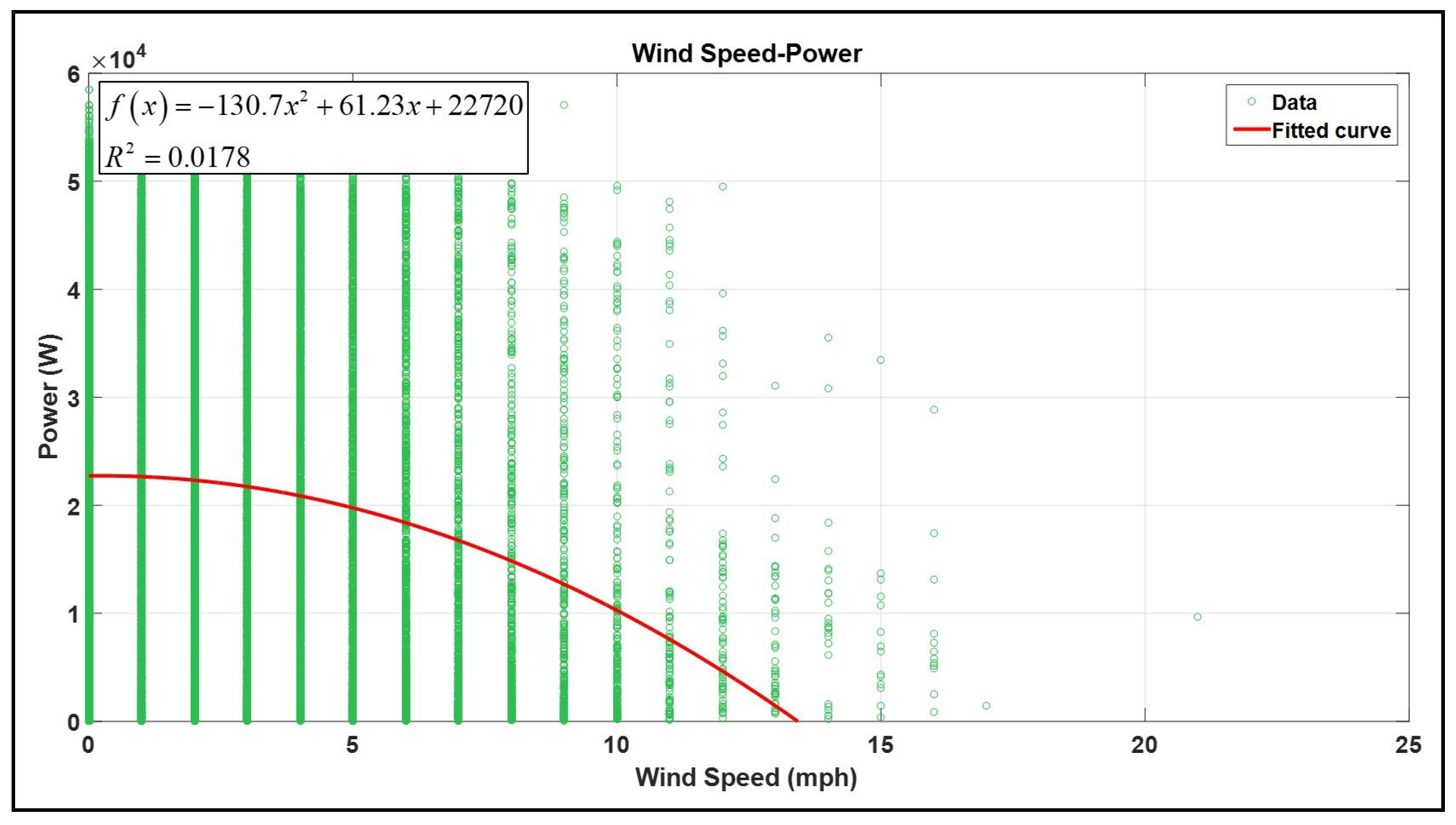
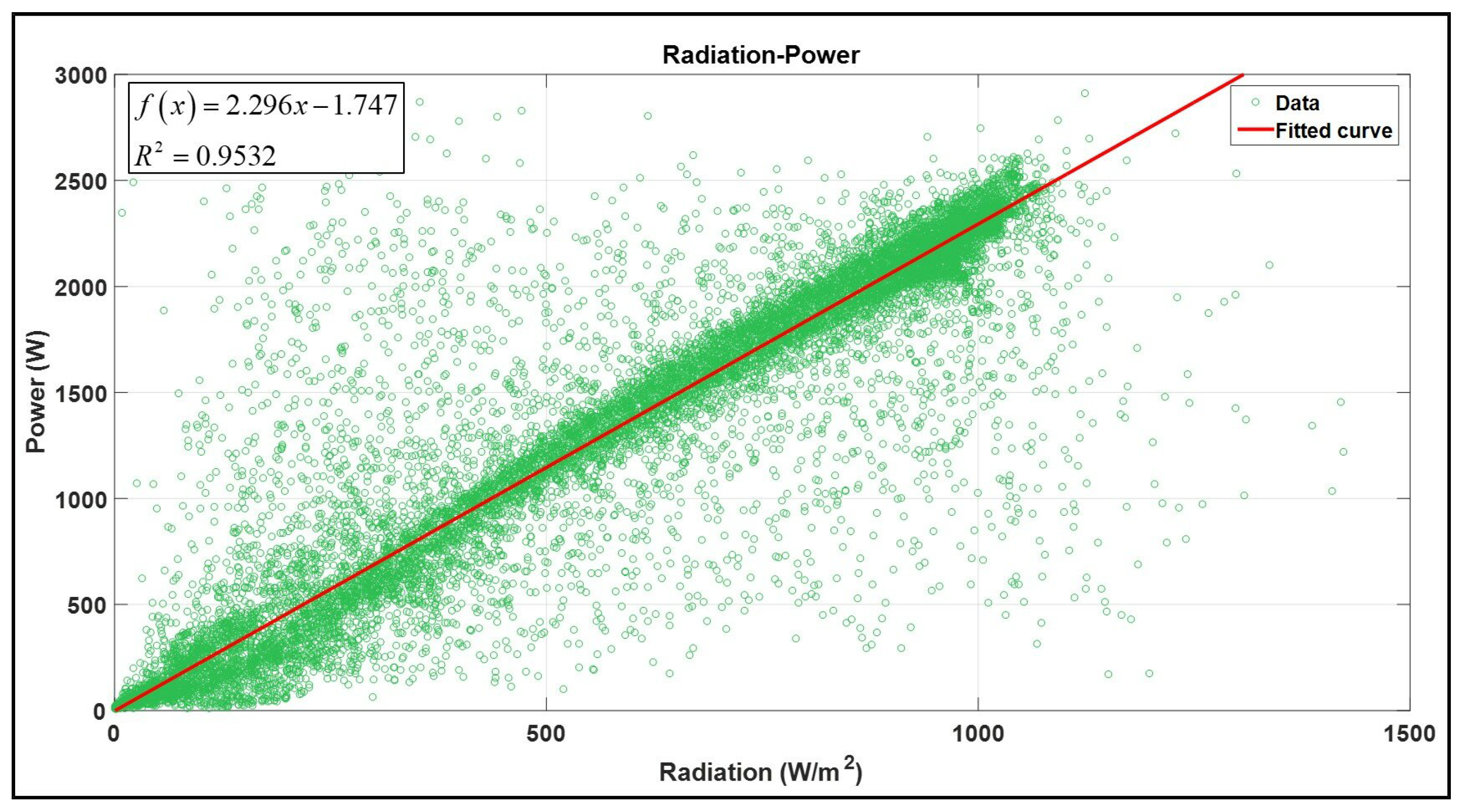
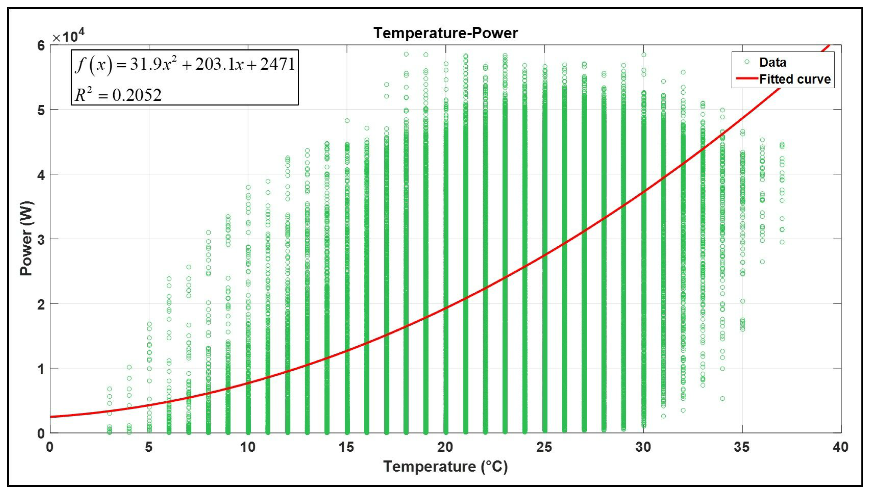
The results showed that solar radiation and daylight time are relevant in estimating the electric power, with solar radiation being the one with the most influence over the photovoltaic power generation; nonetheless, temperature, wind speed, and daylight hour affect this process, with their inclusion being fundamental in the analysis to achieve a proper electric power estimation.

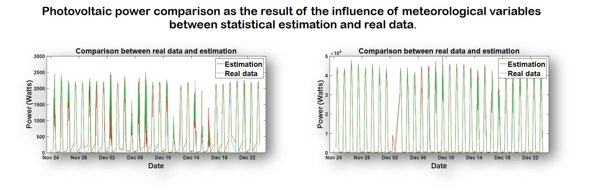
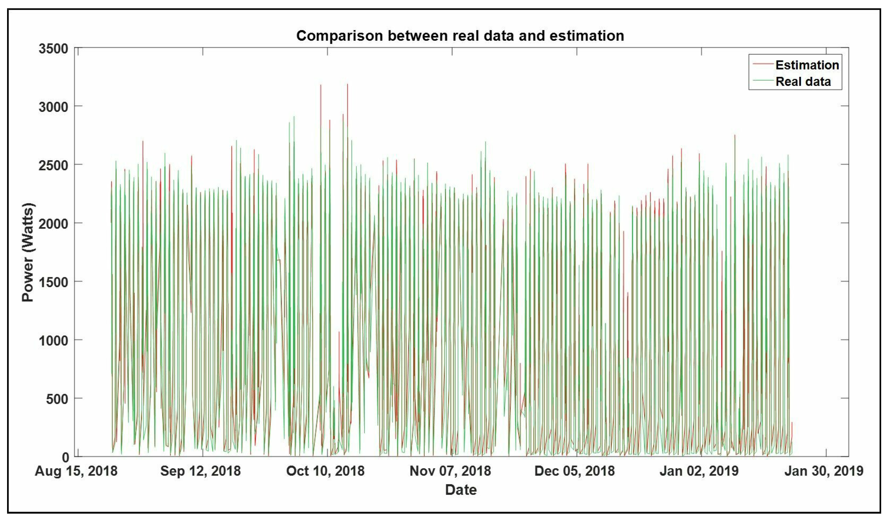
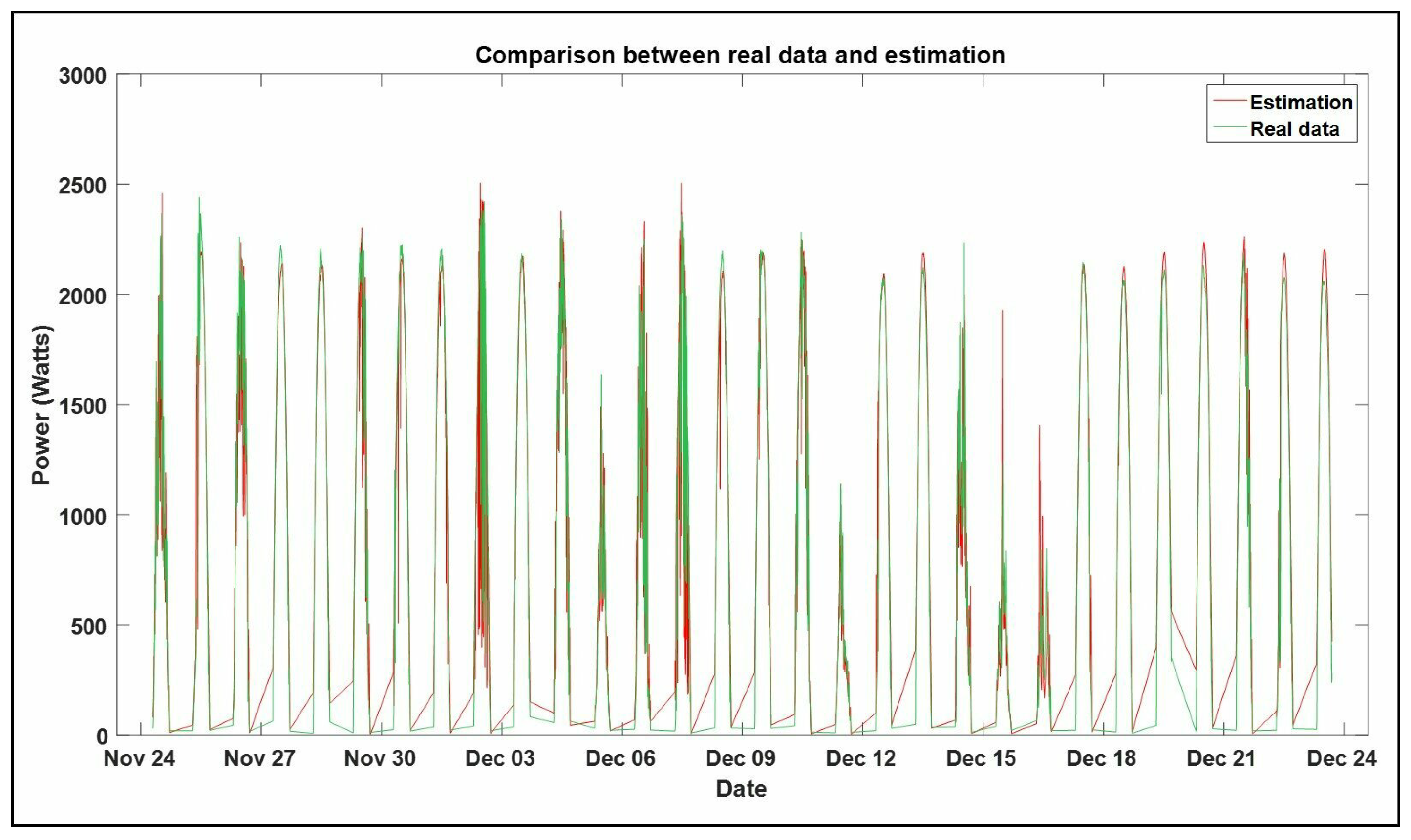
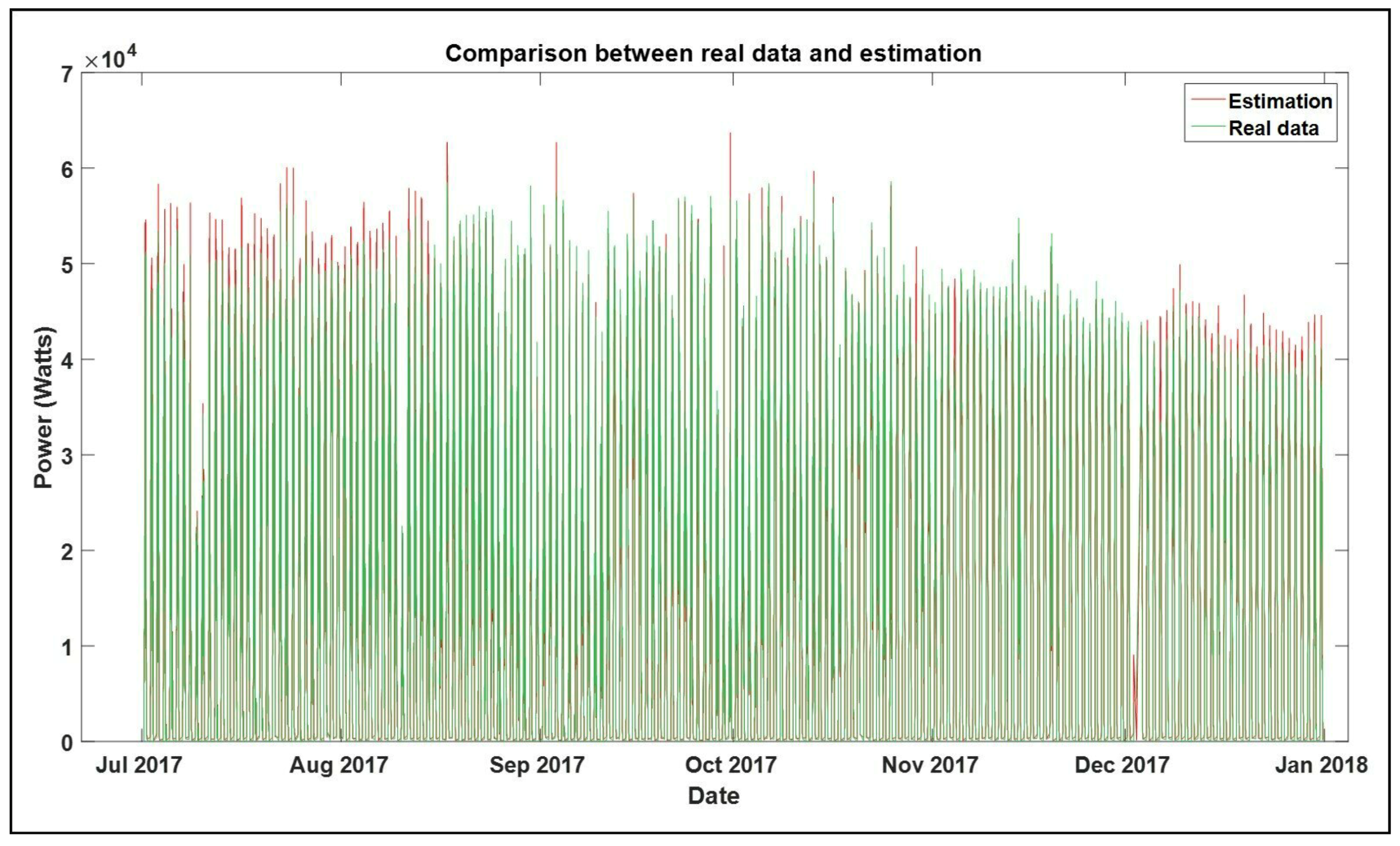
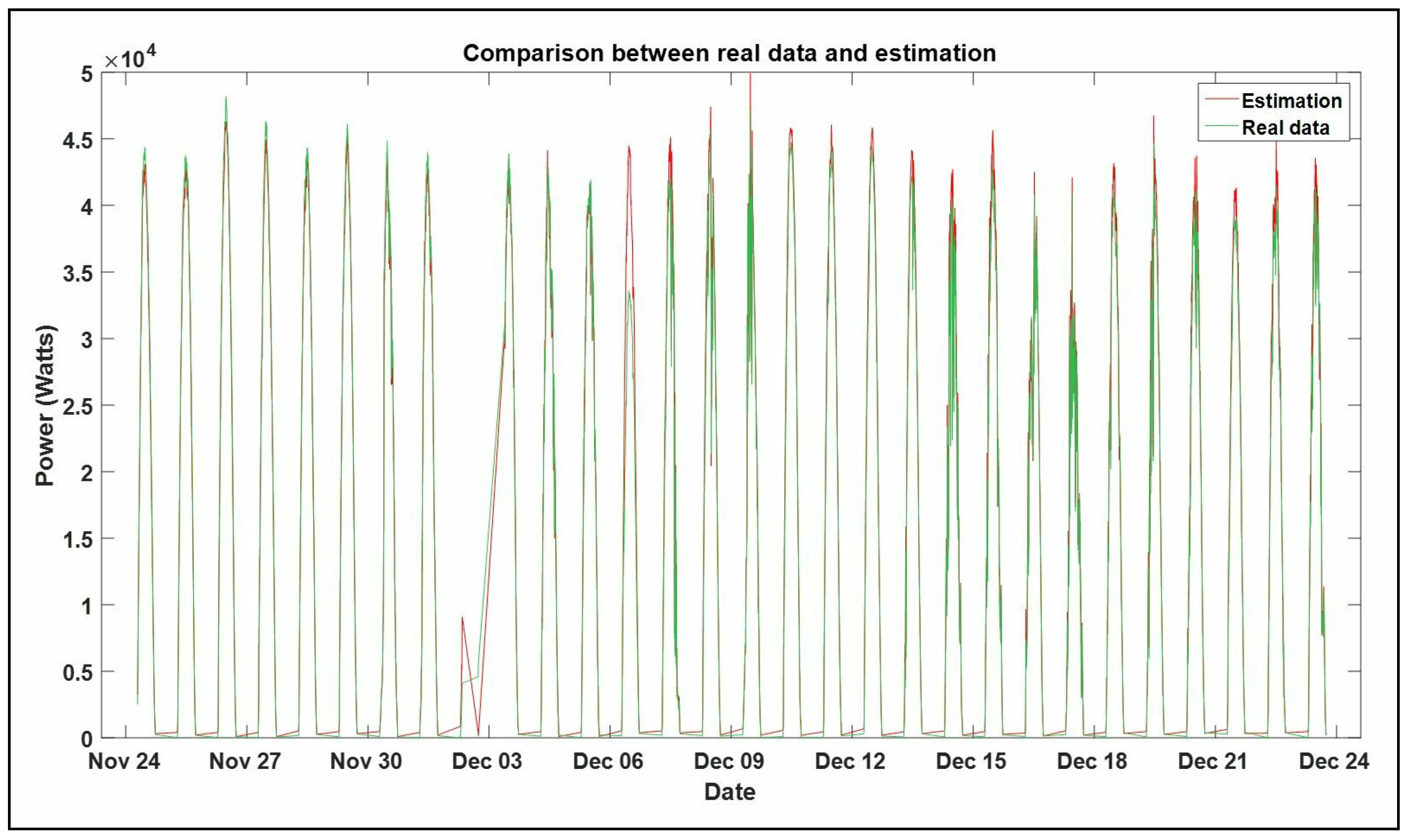
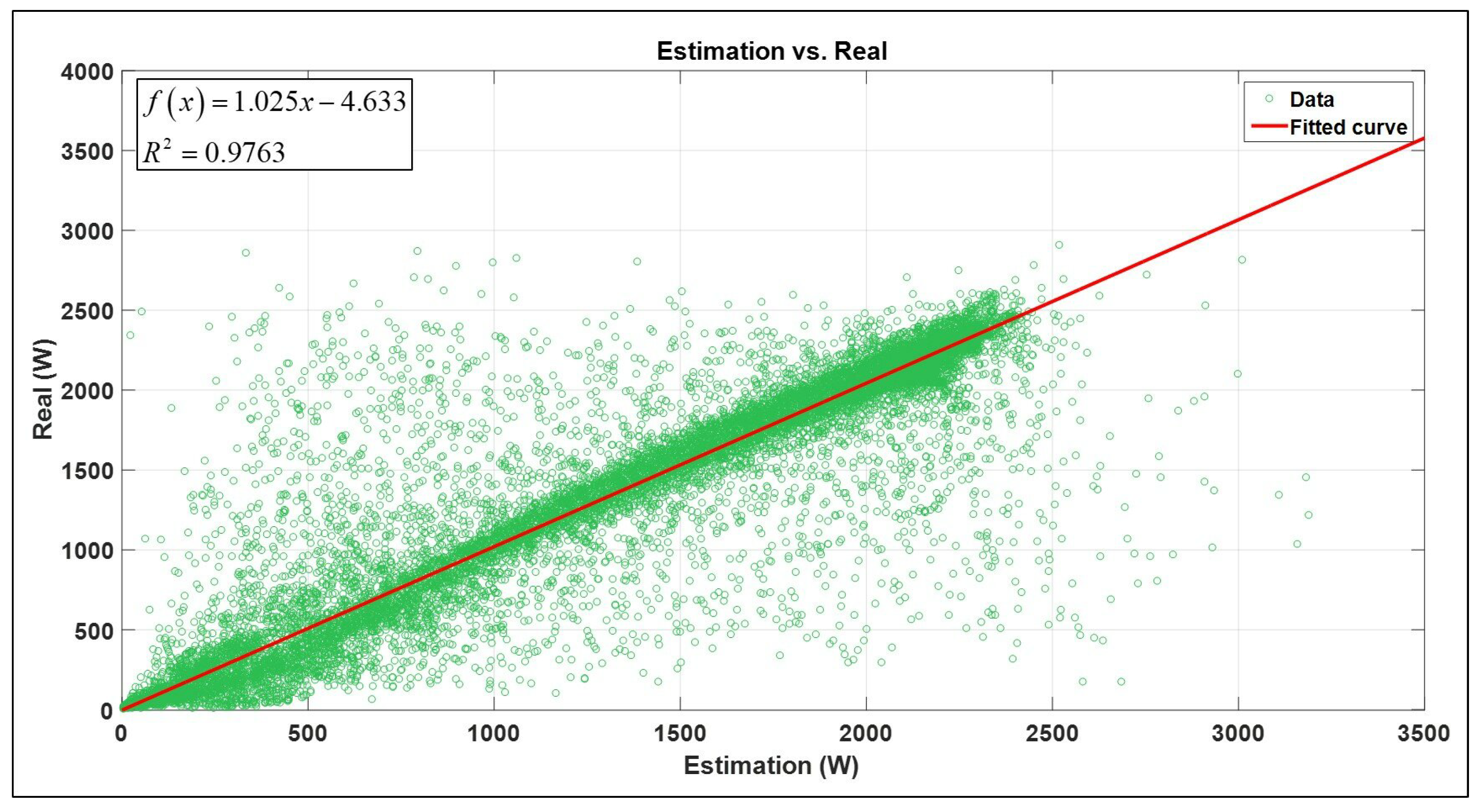
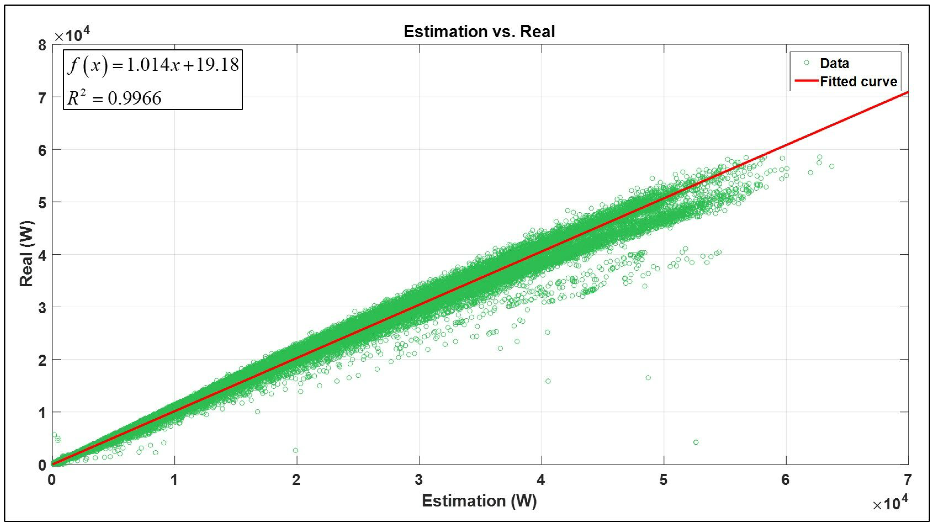
According to Figure 9 and Figure 16, an acceptable approximation between the statistical simulation results and real-time power generation has achieved. This is proven both by Table 8, where 97.63% of the estimation results matches with the real data for HS and 99.66% match for MCS, and by Table 9, achieving overall error values no greater than 7% and 2% for HS and MCS, respectively. An observable relationship between the determination coefficient values and error results is clear, concluding that the percentage error will be lower while $R^2$ is higher.

Several causes could perturb the correlation, resulting in a wider dispersion, with the weather conditions as the most important for this study. Contrary to Mexico City, Hermosillo has abrupt changes in climate throughout the year, reaching temperatures around 50 °C and 0 °C in summer and winter, respectively, as well as sudden weather changes from a sunny day to a cloudy or even a rainy day within hours.

However, according to the above and even if the results have a satisfactory behavior, by definition, a statistical estimation will always have an error value. Nevertheless, these error values can be reduced, increasing the gathered input data or by other alternative methods such as intelligent systems which have proven to be an efficient methodology [53,54,55,56]. The above will be discussed elsewhere.

References

1. D’Adamo, I. The Profitability of Residential Photovoltaic Systems. A New Scheme of Subsidies Based on the Price of CO2 in a Developed PV Market. Soc. Sci. 2018, 7, 148. [Google Scholar] [CrossRef]
2. SEIA. Solar Energy Industries Association. 2018. Available online: https://www.seia.org/initiative-topics/solar-technologies (accessed on 12 April 2019).
3. Järvelä, M.; Valkealahti, S. Ideal operation of a photovoltaic power plant equipped with an energy storage system on electricity market. Appl. Sci. 2017, 7, 749. [Google Scholar] [CrossRef]
4. Awan, A.B.; Zubair, M.; Abokhalil, A.G. Solar energy resource analysis and evaluation of photovoltaic system performance in various regions of Saudi Arabia. Sustainability 2018, 10, 1129. [Google Scholar] [CrossRef]
5. Zahedi, A. Solar photovoltaic (PV) energy; latest developments in the building integrated and hybrid PV systems. Renew. Energy 2006, 31, 711–718. [Google Scholar] [CrossRef]
6. Perea-Moreno, A.J.; Hernandez-Escobedo, Q.; Garrido, J.; Verdugo-Diaz, J.D. Stand-Alone Photovoltaic System Assessment in Warmer Urban Areas in Mexico. Energies 2018, 11, 284. [Google Scholar] [CrossRef]
7. Trujillo-Camacho, M.; García-Gómez, C.; Hinojosa-Palafox, J.; Castillón-Barraza, F. Evaluación de compositos TiO2/clinoptilolita en la fotodegradación del tinte MV-2B en un reactor-concentrador solar cpc. Revista Mexicana de Ingeniería química 2010, 9, 139–149. [Google Scholar]
8. López-Sosa, L.; Hernández-Ramírez, L.; González-Avilés, M.; Servín-Campuzano, H.; Zárate-Medina, J. Desarrollo de un recubrimiento absorbente solar de bajo costo basado en hollín de biomasa forestal: Caracterización térmica y aplicación en un sistema de cocción solar. Revista Mexicana de Ingeniería Química 2018, 17, 651–668. [Google Scholar] [CrossRef]
9. González-Avilés, M.; López-Sosa, L.; Servín-Campuzano, H.; González-Pérez, D. Adopción tecnológica sustentable de cocinas solares en comunidades indígenas y rurales de Michoacán. Revista Mexicana de Ingeniería Química 2017, 16, 273–282. [Google Scholar]
10. Saga, T. Crystalline and Polycrystalline Silicon PV Technology. NPG Asia Mater. 2010, 2, 96–102. [Google Scholar] [CrossRef]
11. Kazem, H.A.; Yousif, J.H.; Chaichan, M.T. Modeling of daily solar energy system prediction using support vector machine for Oman. Int. J. Appl. Eng. Res. 2016, 11, 10166–10172. [Google Scholar]
12. Zhang, W.-T.; Wang, S.; Du, X.-H. Research of power prediction about photovoltaic power system: Based on BP neural network. J. Environ. Prot. Ecol. 2017, 18, 1614–1623. [Google Scholar]
13. Shin, H.; Geem, Z.W. Optimal Design of a Residential Photovoltaic Renewable System in South Korea. Appl. Sci. 2019, 9, 1138. [Google Scholar] [CrossRef]
14. Hogg, D.C.; Decker, M.; Guiraud, F.; Earnshaw, K.; Merritt, D.; Moran, K.; Sweezy, W.; Strauch, R.; Westwater, E.; Little, C. An automatic profiler of the temperature, wind and humidity in the troposphere. J. Clim. Appl. Meteorol. 1983, 22, 807–831. [Google Scholar] [CrossRef]
15. Lawrence, M.G. The relationship between relative humidity and the dewpoint temperature in moist air: A simple conversion and applications. Bul. Am. Meteorol. Soc. 2005, 86, 225–234. [Google Scholar] [CrossRef]
16. Dudley, B. BP Energy Outlook 2040. BP plc 2019. Available online: http://oilproduction.net/files/OilProduction-bp-energy-outlook-2019.pdf (accessed on 12 April 2019).
17. IRENA. Renewable Power Generation Costs in 2017; International Renewable Energy Agency: Abu Dhabi, UAE, 2018; Available online: https://www.irena.org/-/media/Files/IRENA/Agency/Publication/2018/Jan/IRENA_2017_Power_Costs_2018.pdf (accessed on 12 April 2019).
18. Rasero, C.M. Energía Solar Fotovoltaica. Energía Solar Fotovoltaica, Situación Actual 2011. Available online: https://static.eoi.es/savia/documents/componente75553.pdf (accessed on 12 April 2019).
19. Philibert, C. Solar Energy Perspectives; OECD: Paris, France, 2011. [Google Scholar]
20. Elshurafa, A.M.; Albardi, S.R.; Bigerna, S.; Bollino, C.A. Estimating the learning curve of solar PV balance–of–system for over 20 countries: Implications and policy recommendations. J. Clean. Prod. 2018, 196, 122–134. [Google Scholar] [CrossRef]
21. Nemet, G.F.; O’Shaughnessy, E.; Wiser, R.; Darghouth, N.; Barbose, G.; Gillingham, K.; Rai, V. Characteristics of low-priced solar PV systems in the US. Appl. Energy 2017, 187, 501–513. [Google Scholar] [CrossRef]
22. Acceso a Datos de Radiación Solar en España. 2018. Available online: http://www.adrase.com (accessed on 12 April 2019).
23. The World Bank, Solar Resource Data: Solargis, World. 2017. Available online: https://globalsolaratlas.info/downloads/world (accessed on 12 April 2019).
24. The World Bank, Solar Resource Data: Solargis, Mexico. 2017. Available online: https://globalsolaratlas.info/downloads/mexico (accessed on 12 April 2019).
25. Yaneva, M.; Tisheva, P.; Tsanova, T. Mirecweek—The Big Mexico Renewable Energy Report. 2018. Available online: http://www.awex-export.be/files/library/Infos-sectorielles/Ameriques/2017/MEXIQUE/Mirec-Report-2018-The-BIG-Mexico-renewable-energy-report-ENG.pdf (accessed on 12 April 2019).
26. Della Ceca, L.; Micheletti, M.; Freire, M.; Garcia, B.; Mancilla, A.; Salum, G.; Crinó, E.; Piacentini, R. Solar and Climatic High Performance Factors for the Placement of Solar Power Plants in Argentina Andes Sites—Comparison With African and Asian Sites. J. Sol. Energy Eng. 2019, 141, 041004. [Google Scholar] [CrossRef]
27. Sağlam, Ş. Meteorological parameters effects on solar energy power generation. WSEAS Trans. Circuits Syst. 2010, 9, 637–649. [Google Scholar]
28. Nam, S.; Hur, J. Probabilistic Forecasting Model of Solar Power Outputs Based on the Naïve Bayes Classifier and Kriging Models. Energies 2018, 11, 2982. [Google Scholar] [CrossRef]
29. Ding, M.; Wang, L.; Bi, R. An ANN-based approach for forecasting the power output of photovoltaic system. Procedia Environ. Sci. 2011, 11, 1308–1315. [Google Scholar] [CrossRef]
30. Horan, W.; Shawe, R.; O’Regan, B. Ireland’s Transition towards a Low Carbon Society: The Leadership Role of Higher Education Institutions in Solar Photovoltaic Niche Development. Sustainability 2019, 11, 558. [Google Scholar] [CrossRef]
31. Viscidi, L. Mexico’s Renewable Energy Future. 2018. Available online: https://www.wilsoncenter.org/sites/default/files/mexico_renewable_energy_future_0.pdf (accessed on 12 April 2019).
32. SENER. Prospectivas de Energías Renovables 2012–2026. 2012. Available online: https://www.gob.mx/cms/uploads/attachment/file/62954/Prospectiva_de_Energ_as_Renovables_2012-2026.pdf (accessed on 12 April 2019).
33. Gordon, G.; Tibshirani, R. Gradient descent revisited. Optimization 2012, 10, 725. [Google Scholar]
34. Hernández, L.; Baladrón, C.; Aguiar, J.M.; Calavia, L.; Carro, B.; Sánchez-Esguevillas, A.; Cook, D.J.; Chinarro, D.; Gómez, J. A study of the relationship between weather variables and electric power demand inside a smart grid/smart world framework. Sensors 2012, 12, 11571–11591. [Google Scholar] [CrossRef]
35. Ooi, S.C.; Mardiana, A.; Yusup, Y. Analysing Meteorological Variables, Energy Consumption and Occupant Behaviour in an Office Building in Hot-Humid Climate Zone. Int. J. Sci. Res. IJSR 2015, 4, 88–93. [Google Scholar]
36. Hor, C.L.; Watson, S.J.; Majithia, S. Analyzing the impact of weather variables on monthly electricity demand. IEEE Trans. Power Syst. 2005, 20, 2078–2085. [Google Scholar] [CrossRef]
37. Mendoza, C. Viabilidad Técnica-Económica de una Central Solar Termoeléctrica de Colectores Cilíndricos Parabólicos para su Implementación de México. UNAM, Marzo. 2012. Available online: http://132.248.52.100:8080/xmlui/handle/132.248.52.100/277 (accessed on 12 April 2019).
38. Benesty, J.; Chen, J.; Huang, Y.; Cohen, I. Pearson correlation coefficient. In Noise Reduction in Speech Processing; Springer: Berlin, Germany, 2009; pp. 1–4. [Google Scholar]
39. Spiegel, M.; Stephens, L. Estadística, 4th ed.; Graw Hill: Contadero, Mexico, 2009; ISBN 978-6-071-51188-1. Available online: https://www.google.com/url?sa=t&rct=j&q=&esrc=s&source=web&cd=1&ved=2ahUKEwj12s7rtLDhAhWB7Z8KHQIiDwAQFjAAegQIAxAC&url=http%3A%2F%2Fensfep.edu.mx%2Fenlinea%2Fpluginfile.php%2F1531%2Fmod_folder%2Fcontent%2F0%2FEstad%25C3%25ADstica.%2520Serie%2520Schaum-%2520 (accessed on 12 April 2019).
40. Taylor, R. Interpretation of the correlation coefficient: A basic review. J. Diagn. Med. Sonogr. 1990, 6, 35–39. [Google Scholar] [CrossRef]
41. Clack, C.T. Modeling solar irradiance and solar PV power output to create a resource assessment using linear multiple multivariate regression. J. Appl. Meteorol. Climatol. 2017, 56, 109–125. [Google Scholar] [CrossRef]
42. Aggarwal, S.; Saini, L. Solar energy prediction using linear and non-linear regularization models: A study on AMS (American Meteorological Society) 2013–14 Solar Energy Prediction Contest. Energy 2014, 78, 247–256. [Google Scholar] [CrossRef]
43. Bairán, J.M.; Marí, A.; Cladera, A. Analysis of shear resisting actions by means of optimization of strut and tie models taking into account crack patterns. Hormigón y acero 2018, 69, 197–206. [Google Scholar] [CrossRef]
44. Arjoune, Y.; Mrabet, Z.; Kaabouch, N. Multi-Attributes, Utility-Based, Channel Quality Ranking Mechanism for Cognitive Radio Networks. Appl. Sci. 2018, 8, 628. [Google Scholar] [CrossRef]
45. Montgomery, D.C. Design and Analysis of Experiments; John Wiley & Sons: Hoboken, NJ, USA, 2017; ISBN 978-1-119-11347-8. Available online: https://www.wiley.com/en-mx/Design+and+Analysis+of+Experiments%2C+9th+Edition-p-9781119113478 (accessed on 12 April 2019).
46. Gardiner, S.K.; Crabb, D.P. Examination of different pointwise linear regression methods for determining visual field progression. Investig. Ophthalmol. Vis. Sci. 2002, 43, 1400–1407. [Google Scholar]
47. Verma, S.; Bartosova, A.; Markus, M.; Cooke, R.; Um, M.J.; Park, D. Quantifying the Role of Large Floods in Riverine Nutrient Loadings Using Linear Regression and Analysis of Covariance. Sustainability 2018, 10, 2876. [Google Scholar] [CrossRef]
48. Ng, A. CS229 Lecture Notes. 2000, Volume 1, pp. 1–3. Available online: http://backspaces.net/temp/ML/CS229.pdf (accessed on 12 April 2019).
49. Google Maps, UNISON. 2019. Available online: https://www.google.com/maps/place/Universidad+de+Sonora+-+UNISON/@23.9391074,-102.172878,2504267m/data=!3m1!1e3!4m5!3m4!1s0x86ce8447973925f7:0xcf527709b7555a3!8m2!3d29.0834761!4d-110.9603621 (accessed on 12 April 2019).
50. Google Maps, CINVESTAV. 2019. Available online: https://www.google.com/maps/place/CINVESTAV+-+IPN/@23.9391074,-102.172878,2504267m/data=!3m1!1e3!4m5!3m4!1s0x85d1f77a076bd911:0x63af0ad86ca91f65!8m2!3d19.5099425!4d-99.129559 (accessed on 12 April 2019).
51. Dev, S.; AlSkaif, T.; Hossari, M.; Godina, R.; Louwen, A.; van Sark, W. Solar Irradiance Forecasting Using Triple Exponential Smoothing. In Proceedings of the 2018 International Conference on Smart Energy Systems and Technologies (SEST), Sevilla, Spain, 10–12 September 2018; pp. 1–6. [Google Scholar]
52. Chai, T.; Draxler, R.R. Root mean square error (RMSE) or mean absolute error (MAE)?—Arguments against avoiding RMSE in the literature. Geosci. Model Dev. 2014, 7, 1247–1250. [Google Scholar] [CrossRef]
53. Peterson, M.G. Intelligent medical systems and the interface with statistics. In Proceedings of the 11th IEEE Symposium on Computer-Based Medical Systems, Lubbock, TX, USA, 12–14 June 1998; p. 300. [Google Scholar]
54. Chen, S.H.; Jakeman, A.J.; Norton, J.P. Artificial intelligence techniques: An introduction to their use for modelling environmental systems. Math. Comput. Simul. 2008, 78, 379–400. [Google Scholar] [CrossRef]
55. Mosavi, A.; Ozturk, P.; Chau, K.w. Flood prediction using machine learning models: Literature review. Water 2018, 10, 1536. [Google Scholar] [CrossRef]
56. Inman, R.H.; Pedro, H.T.; Coimbra, C.F. Solar forecasting methods for renewable energy integration. Prog. Energy Combust. Sci. 2013, 39, 535–576. [Google Scholar] [CrossRef]
Figure 1. The worldwide horizontal solar radiation [23].
Applsci 09 01649 g001
Figure 2. The Mexican solar radiation atlas [24].
Applsci 09 01649 g002
Figure 3. The geographical location of the Hermosillo Site (HS) [49] (29.0843293 N, −110.9583558 W).
Applsci 09 01649 g003
Figure 4. The Power vs. Solar radiation of HS.
Applsci 09 01649 g004
Figure 5. The Power vs. Temperature of HS.
Applsci 09 01649 g005
Figure 6. The Power vs. Wind speed of HS.
Applsci 09 01649 g006
Figure 7. The Power vs. Time of HS.
Applsci 09 01649 g007
Figure 8. The results obtained from HS by gradient descent.
Applsci 09 01649 g008
Figure 9. A close-up of the results from HS.
Applsci 09 01649 g009
Figure 10. The geographical location of Mexico City Site (MCS) [50] (19.5099425 N, −99.1317477 W).
Applsci 09 01649 g010
Figure 11. The Power vs. Solar radiation of MCS.
Applsci 09 01649 g011
Figure 12. The Power vs. Temperature of MCS.
Applsci 09 01649 g012
Figure 13. The Power vs. Wind speed of MCS.
Applsci 09 01649 g013
Figure 14. The Power vs. Time of MCS.
Applsci 09 01649 g014
Figure 15. The results obtained from MCS by gradient descent.
Applsci 09 01649 g015
Figure 16. A close-up of the results from MCS.
Applsci 09 01649 g016
Figure 17. The estimated vs. real photovoltaic power of HS.
Applsci 09 01649 g017
Figure 18. The estimated vs. real photovoltaic power of MCS.
Applsci 09 01649 g018
Figure 19. The difference errors between the high and low values: (a) Error value when measured data is high; (b) Error value when measured data is low.
Applsci 09 01649 g019