Article

Cluster Analysis of Pedestrian Mobile Channels in Measurements and Simulations

1
Key Laboratory of Universal Wireless Communications, Ministry of Education, Beijing University of Posts and Telecommunications, Beijing 100876, China
2
State Key Laboratory of Networking and Switching Technology, Beijing University of Posts and Telecommunications, Beijing 100876, China
*
Author to whom correspondence should be addressed.
Appl. Sci. 2019, 9(5), 886; https://doi.org/10.3390/app9050886
Submission received: 9 January 2019 / Revised: 14 February 2019 / Accepted: 26 February 2019 / Published: 1 March 2019
(This article belongs to the Section Electrical, Electronics and Communications Engineering)

Abstract

:
In wireless communication systems, channels evolve when user terminals move. To further understand channel variation, and especially the evolution of clusters in mobile channels, a set of experiments was designed. First, we performed pedestrian mobile measurements in an urban macro (UMa) scenario at 3.5 GHz, and the K-power means-Kalman filter (KPMKF) algorithm was used for clustering and tracking. By this process, the trajectory of different clusters could clearly be described during measurement. The birth and death rate of clusters per snapshot show that the change of one or two clusters in each snapshot takes more probabilities. In addition, the differences of the cluster lifetime between the clustering process with and without the Kalman filter (KF) algorithm are given to show the effect from the KF. Second, channel simulations were implemented based on the above observed results. The spatial-consistency feature was introduced to get closer to the measured channels, which is based on the primary module of International Mobile Telecommunications-2020 (IMT-2020) channel model. Comparisons among measurements and simulations with and without this feature show that adding this feature improves simulation accuracy. To explore a novel method to characterize clusters during linear movement, a gradient boosted decision-tree (GBDT) algorithm is introduced. It uses the above characteristics of clusters and channel impulse responses (CIRs) as the training and validating dataset. The root mean square error (RMSE) shows that this is promising.

Graphical Abstract

1. Introduction

Research on the channel model is one of the basic works in wireless communication systems. It is an abstract description of wireless propagation characteristics. Researchers in the field of wireless communications have had great interest in channel modelling in various kinds of propagation environments (such as urban, suburb, and indoor) since the 1970s. They focused on how to build a mathematical model based on theoretical and measurement analysis, which approximately simulates real channel conditions. From the 3G to the 4G era, the channel model has already changed from the tapped delay line (TDL) model in M. 1225 [1], which is known as the International Mobile Telecommunications-2000 (IMT-2000) channel model, to geometry-based stochastic channel model (GBSM) in M. 2135 [2], which is known as IMT-Advanced channel model. ITU radiocommunication sector (ITU-R) started the project to draft a new channel model, called IMT-2020, to meet the new requirements in the 5G era, which was published in M. 2412 on October 2017 [3].
As the basis of GBSM models, a cluster can reflect path characteristics in the channels, and their variation over time can show channel time-variant and spatial-variant features in mobile scenarios. Many measurements in different scenarios were conducted, followed by theoretical analysis to study the statistical modelling of clusters. Reference [4] proposes the average number of clusters in indoor office environments, which can reflect the active number of clusters in different positions. Reference [5] shows the lifetimes of clusters in indoor-to-outdoor and outdoor-to-indoor environments, while Reference [6] reports them in an indoor hall environment. Moreover, how to continuously parameterize the clusters, and track and identify them in mobile channels have been considered in many studies. Reference [7] built an evolution model of the number of clusters from dynamic double-directional measurements in an indoor environment, and uses cluster-level parameters to describe the mobile channels. Reference [8] gives a Kuhn-Munkres-based method to model the evolution of clusters that is based on simulations of the 3rd Generation Partnership Project (3GPP) channel model.
However, cluster-tracking statistical analysis to massive Multiple Input Multiple Output (MIMO) pedestrian mobile measurements, which can detect richer scatterers in environments, needs to be further studied. Although we performed cluster analysis in References [9,10] with the K-power means (KPM) algorithm, it can only independently do clustering in each snapshot. The relationships of clusters between neighboring snapshots and their birth–death process are unknown, nor does the corresponding validation work on the primary module of the IMT-2020 channel model.
Considering this, we focused on better presenting the evolution of clusters in mobile channels in both measurements and simulations. Thus, the contributions of this paper are summarized as follows.
  • The KPM-Kalman filter (KPMKF) algorithm is used for massive MIMO urban macro (UMa) pedestrian mobile scenario measurement. With this method, evolution including the birth and death rate and lifetime of clusters can be clearly shown. The difference of clustering results with and without Kalman filter (KF) part is also shown.
  • The spatial-consistency feature is introduced and implemented to complement the primary module of the IMT-2020 channel model. It makes the channel evolve smoothly without discontinuity when Transmitter (Tx)/Receiver (Rx) moves. With this feature, cluster characteristics are highly correlated among neighboring moving locations, which is closer to real conditions. In the meantime, comparisons among between measurements and simulations with and without this feature are shown.
  • Inspired by Reference [11], a novel clustering method based on the gradient boosted decision-tree (GBDT) algorithm is explored to train and validate the results from the above measurements and simulations. It was proven to be an effective way to characterize cluster evolution in certain scenarios during linear movement.
The remainder of this paper is organized as follows. Section 2 gives details of the measurement setup, the data process, and the analysis results. In Section 3, generation procedures of channel simulations by the IMT-2020 channel model with the spatial-consistency feature are described, as are the simulation results. Section 4 gives the framework of the GBDT-based model, and the validated results by the GBDT-based model. Finally, conclusions are drawn in Section 5.

2. Cluster Tracking in Mobile Measurements

In contrast to channels from a conventional MIMO system, massive MIMO systems give richer channel information [12,13,14]. Considering this, a virtual massive MIMO pedestrian mobile measurement campaign was performed to observe cluster evolution. To characterize the evolution process of clusters, which is greatly influential on cluster number in mobile channels, the tracking algorithm was considered. All details of the measurement setup, the data extraction and processing method, and data analysis are shown in the following.

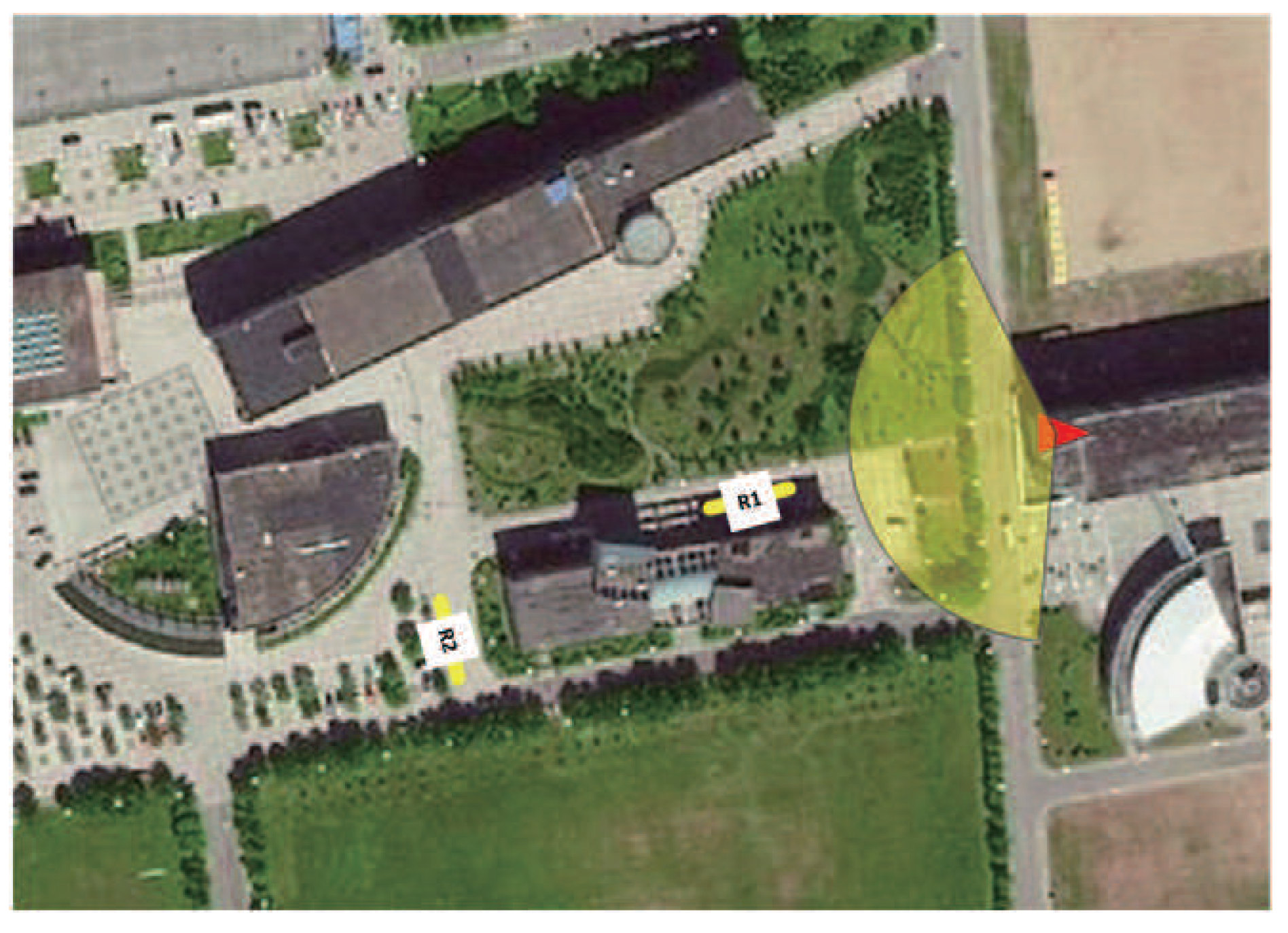
2.1. Measurement Setup and Data Processing

Channel measurement took place in a square at the Beijing University of Posts and Telecommunications (see Figure 1), which can be seen as a typical UMa scenario. The used channel sounder had a carrier frequency of 3.5 GHz and 200 MHz bandwidth and collected the raw data of channel impulse responses (CIRs). A 32-element uniform planar array (UPA) was used at the Tx side, shown in Figure 2a. At the Rx side, the dual-polarized omnidirectional array (ODA) was equipped with a 56-element antenna. In this case, Antennas 1–16 were chosen for the measurement campaign (see Figure 2b). Measurement details are listed in Table 1.
During measurement, the Rx moved along with the 8 m rail at a constant speed of 1.4 m/s (pedestrian speed). The Tx side was set on the roof of a teaching building. Two measurement routes were in line-of-sight (LoS) and non-line-of-sight (NLoS) conditions, respectively. Route R1, moving from east to west, had LoS conditions. R2, moving from north to south, had NLoS conditions, and was mainly blocked by the building and shrubs.
To form the massive MIMO array with 256 antennas, a virtual-measurement method was adopted. Figure 3 shows the scheme of 256-element combining antenna array, giving 8 continuous positions. After collecting the raw data, we combined the 8 CIRs into one group.
h i ( t , τ ) = n = 1 N α n ( i ) e j ϕ n ( i ) ( t ) δ ( τ τ n ( i ) ) ,
where i = 1 , 2 , , 8 . α n ( i ) , ϕ n ( i ) ( t ) and τ n ( i ) represent the amplitude, phase, and delay of the nth sample in the time domain at the ith angle bin, respectively. N is the number of collected CIRs.
Then, CIRs are combined into one group as
h v i r t u a l ( t , τ ) = [ h 1 ( t , τ ) , h 2 ( t , τ ) , , h 8 ( t , τ ) ] ,
where h v i r t u a l ( t , τ ) can be considered as the equivalent CIR collected from a 256 antenna UPA. The rationality of this method was proven in Reference [15]. It shows that there is a good match between the power delay profile (PDP) calculated from CIRs collected from the measurement campaigns and the combined CIRs. Furthermore, spatial angular characteristics, including elevation angle of departure (EoD), azimuth angle of departure (AoD), elevation angle of arrival (EoA), and azimuth angle of arrival (AoA), which were estimated from the combination, fit well with those from the measurement campaigns.
After combining the 8 groups of CIRs sequences into one group of sequences, the space-alternating generalized expectation maximization (SAGE) algorithm was used to estimate the channel parameters from the raw data [16], which provides a joint estimation of parameter set θ l = { τ l , f d , l , Φ l , Ω l , α l } , l = { 1 , , L } . τ l , f d , l , Φ l , Ω l , and α l denote propagation delay, the Doppler shift, the AoD, the AoA, and polarization of the lth propagation subpath, respectively. Specifically, Φ l = [ θ T , l , ϕ T , l ] , Ω l = [ θ R , l , ϕ R , l ] , where θ T , l , ϕ T , l , θ R , l and ϕ R , l denote the EoD, AoD, EoA, and AoA, respectively. The number of estimated multipath components (MPCs) was set to 100 in each snapshot.
With this information on the MPC level, we could cluster them with similar parameters, e.g., AoA, AoD, and delay. In References [9,10], we only used KPM for clustering, and the process worked independently in each snapshot. Although the evolution of clusters could be observed along with the movement, the relationships among continuous snapshots and statistical analysis cannot be seen by KPM. For parameterizing clusters in mobile channels over time and showing their continuous evolution, KPM was used for clustering and KF was used for tracking [17,18].
The flowchart of the KPMKF algorithm is shown in Figure 4, where X ( n ) is the data matrix of 100 MPCs in an n t h snapshot. X ( n ) = [ x 1 ( n ) , x 2 ( n ) , , x i ( n ) , , x 100 ( n ) ] T , x i ( n ) = [ τ i ( n ) θ T x , i ( n ) ϕ T x , i ( n ) θ R x , i ( n ) ϕ R x , i ( n ) ] , P ( n ) represents the matrix of MPC power. State model g c ( n ) = [ τ i ( n ) θ T x , i ( n ) ϕ T x , i ( n ) θ R x , i ( n ) ϕ R x , i ( n ) Δ τ i ( n ) Δ θ T x , i ( n ) Δ ϕ T x , i ( n ) Δ θ R x , i ( n ) Δ ϕ R x , i ( n ) ] T . The matrix of cluster centroids is μ c ( n ) = [ τ c ( n ) θ T x , c ( n ) ϕ T x , c ( n ) θ R x , c ( n ) ϕ R x , c ( n ) ] T .
In this framework, X ( 1 ) and P ( 1 ) were used as initial input to the KPM part. After clustering in the first snapshot, we obtained μ c ( 1 ) and initial state g c ( 1 | 0 ) . Then, KF uses these two parameters to update the state as g c ( 1 | 1 ) , and predict the state as g c ( 2 | 1 ) for the second snapshot. Then, we input the X ( 2 ) and P ( 2 ) to perform clustering in the second snapshot. Then, KF takes both the predicted and KPM-processed values into consideration to get g c ( 3 | 2 ) . The process cycle keeps working until the last snapshot is considered. The details of KPM and KF are given as follows, respectively.

2.1.1. K-Power Means Part

Generally, KPM minimizes the total weight of multipath component distance (MCD) to the corresponding cluster centroid by iterations [19]. The MCD between the ith and jth MPC is calculated by
M C D i j = M C D τ , i j 2 + M C D T x , i j 2 + M C D R x , i j 2
of which M C D τ , i j is the delay distance given as follows:
M C D τ , i j = η · τ i τ j Δ τ · τ s d Δ τ
η is a scaling factor to adjust the weight of delay in the distance function. Δ τ means the range of delay, and Δ τ = m a x i , j τ i τ j . τ s d is the standard deviation of delay.
Angle distance M C D T x / R x , i j is given as
M C D T x / R x , i j = 1 2 s i n ( θ T x / R x , i ) c o s ( ϕ T x / R x , i ) s i n ( θ T x / R x , i ) s i n ( ϕ T x / R x , i ) c o s ( θ T x / R x , i ) s i n ( θ T x / R x , j ) c o s ( ϕ T x / R x , j ) s i n ( θ T x / R x , j ) s i n ( ϕ T x / R x , j ) c o s ( θ T x / R x , j )
First, we randomly choose the K positions of cluster centroids [ c 1 ( 0 ) , c 2 ( 0 ) , , c K ( 0 ) ] as the initial state. Then, we start iterations in the following steps:
  • Assign MPCs to cluster centroids and store indices:
    F l ( i ) = a r g m i n ( P l · M C D ( X l , c k ( i 1 ) ) ) F ( i ) = [ F 1 ( i ) , F 2 ( i ) , , F L ( i ) ] , C k i = I n d i c e s l ( F l i = k )
    where F l ( i ) is the cluster index of the lth MPC in the ith iteration. C k i is the set of MPCs indices belonging to the kth cluster in the ith iteration.
  • Recalculate positions of cluster centroids c k ( i ) from the allocated MPCs to coincide with the clusters’ centers of gravity:
    c k i = j C k i ( P j · X j ) j C k i P j
  • If c k ( i ) = c k ( i 1 ) for all k = 1 , , K , then we go out of the iterations. Otherwise, we keep performing iterations up to the setting maximum iteration times.
Finally, we obtain the optimal cluster set. Here, the maximum iteration times were set as 100.

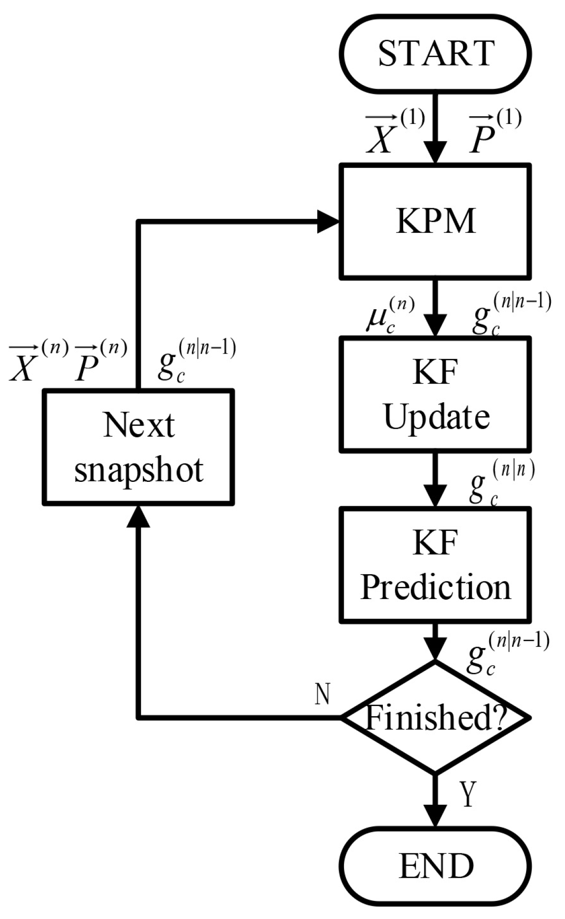
2.1.2. Kalman Filter Part

State model g c ( n ) is assumed as follows:
g c ( n ) = Φ g c ( n 1 ) + N 1 = I 5 1 1 0 1 · g c ( n 1 ) + Δ ( n | n 1 ) + N 1
where Φ is the state-transition matrix, I i is the identity matrix with i dimensions, ⊗ is the product of the Kronecker matrix, N 1 is the state noise, and Δ ( n | n 1 ) is the gap-compensation matrix, which is given as
Δ ( n | n 1 ) = [ Δ τ i ( n | n 1 ) Δ θ T x , i ( n | n 1 ) Δ ϕ T x , i ( n | n 1 ) Δ θ R x , i ( n | n 1 ) Δ ϕ R x , i ( n | n 1 ) ] [ 0 1 ] T
The observation model is the information of cluster centroids themselves, μ c ( n ) , which is given as
μ c ( n ) = J g c ( n ) + N 2 = I 5 [ 1 0 ] · g c ( n ) + N 2
where N 2 is the observation noise.
The update step of KF is
K k = P Φ ( n | n 1 ) J T ( J P Φ ( n | n 1 ) J T + R ) 1
g C ( n ) g C ( n | n 1 ) + K k ( μ C ( n ) J g C ( n | n 1 ) )
P Φ ( n ) = ( I K k J ) P Φ ( n | n 1 )
The predict step of KF is
g C ( n | n 1 ) Φ g C ( n 1 ) + Δ ( n | n 1 )
P Φ ( n | n 1 ) = Φ P Φ ( n 1 ) Φ T + Q
where P Φ is the error covariance matrix, K k is the optimal Kalman gain, and Q and R are the noise-covariance matrices.
It is noted that the state space model was chosen for the basic model description since it is suitable for linear movement [18]. Therefore, in the processing, Q, R, and P Φ ( 0 ) were set as the identify matrices.

2.2. Clustering and Tracking Results

The spatial distributions of clusters in LoS and NLoS conditions are shown in Figure 5a,b, respectively. In the LoS condition, one cluster survives during the whole movement near the main path on 0 . In the NLoS condition, on the other hand, no cluster can keep surviving during the whole movement. Some clusters with a shorter lifetime can be observed. Their angles and power smoothly change with the movement. It is noted that those clusters with less than 5% normalized power were removed in the figures to make the main contributed clusters clearer for observation. Ignored clusters’ contributions to the channels are slight, and most of them have a short lifetime that only exists only in 1 snapshot. However, in the following statistical works, all of them are considered.
From Figure 5c, we see the birth and death histograms of clusters per snapshot that were calculated, which show the birth and death rate of clusters of all snapshots during movement. The total number of newly appeared clusters per snapshot is slightly larger than that of newly disappeared clusters per snapshot. Obviously, the change of 1 or 2 clusters per snapshot takes more probabilities. The polynomial fitting of both birth and death rate is also given in the figure.
The cumulative density functions (CDFs) of cluster lifetime distances are shown in Figure 5d. In our former work, Reference [9], the sizes of visibility regions (VRs) are calculated from the results by KPM algorithm, which are shown in blue and green curves in this figure. VR is a concept proposed in COST 2100 [20], which is an indicator of where corresponding clusters are active. In linear mobile measurements, VR diameters are the same as the lifetime distances of clusters. From this figure, we can see the effect of the newly introduced KF algorithm. Especially in LoS, most clusters show shorter lifetime distances, less than 1 m. In addition, the corresponding log-normal fit is given.

3. Mobile Channel Simulations by IMT-2020 Channel Model

The channel model is used to meet the requirements of evaluating IMT-2020 candidate radio-interface technologies (RITs) by allowing the realistic modelling of propagation conditions for radio transmissions in different environments [3]. Generally, a GBSM channel model is built in a 2D/3D co-ordinate system. The path loss model, shadow fading, small-scale parameters of clusters in typical scenarios (such as indoor hotspots (InH), UMa, urban micro (UMi), and rural macro (RMa)) are analyzed and collected from many empirical measurements. This can simulate and reproduce channel information that is similar with that in real conditions. In this section, the IMT-2020 channel model is used to simulate the measured channels. It follows the typical GBSM channel-model procedures in ITU-R M. 2135 [2], 3GPP TR 38. 900 [21], and TR 36. 873 [22]. To get closer to the mobile channels, the spatial-consistency feature was implemented, which is based on the primary module of the IMT-2020 channel model. Simulation results, including moving trajectory, path loss model, and angle evolution of clusters, are given, as are comparisons between measurements and simulations with and without this feature.

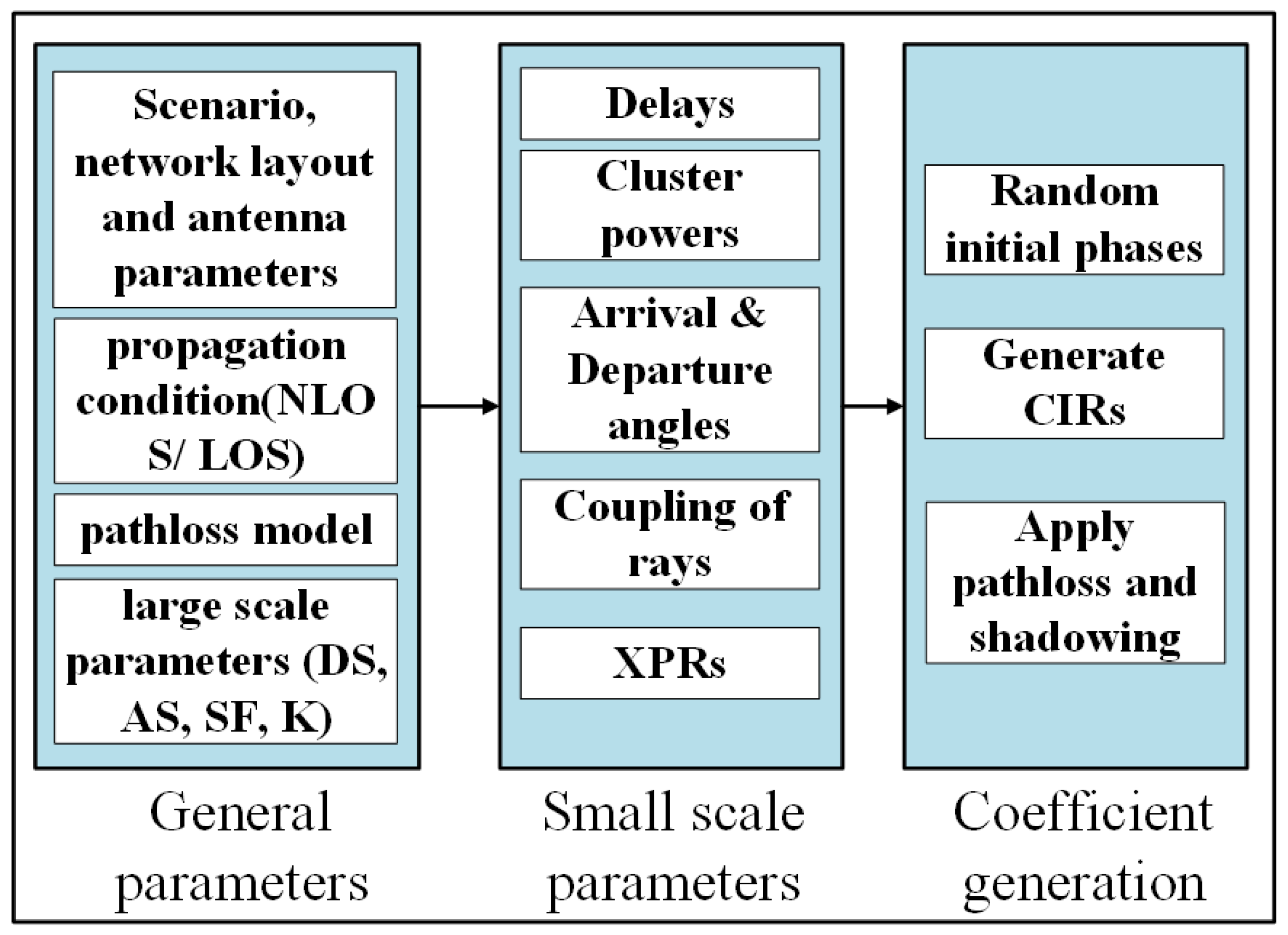
3.1. Simulation Generation Procedures

The generation of a channel model is divided in three main parts: general parameters, small-scale parameters, and coefficient generation (see Figure 6).
The first part, the generation of general parameters, includes the initial setup of the whole system, and how to generate the corresponding path loss model and its large-scale parameters. Users must choose one of four typical scenarios: InH, UMa, UMi, and RMa. Base station (BS) and user terminal (UT) antenna-array details need to be set, such as the number of antennas, 3D locations, antenna field patterns, and array geometries. The speed and direction of UT motion, center frequency, and bandwidth must be set, too. Then, the corresponding path loss model with the formulas is formed. Finally, large-scale parameters are calculated, including root mean square delay spread, root mean square angular spreads, Ricean K-factor, and shadow fading.
In the second part, small-scale parameters are calculated. This is a group of parameters that represents the characteristics of dynamic clusters in the model, which include the delay, power, AoA, AoD, EoA, and EoD of each cluster. After this step, we can obtain the full information of the model clusters.
In the third part, initial phases are generated randomly at first. Each ray m of cluster n has four initial phases: Φ n , m θ θ , Φ n , m θ ϕ , Φ n , m ϕ θ , Φ n , m ϕ ϕ for four different polarization combinations ( θ θ , θ ϕ , ϕ θ , ϕ ϕ ). Their distribution is uniform within ( π , π ). Then, CIRs, also known as channel coefficients, are calculated. Finally, we apply path loss and shadowing to the CIR generation formula. For a channel simulation with S antenna elements at the Tx side and U antenna elements at the Rx side, the equation of generating a channel CIR is expressed as
H u , s , n ( t ) = P n M m = 1 M F r x , u , θ ( θ n , m , E o A , ϕ n , m , A o A ) F r x , u , ϕ ( θ n , m , E o A , ϕ n , m , A o A ) T e x p ( j Φ n , m θ θ ) κ 1 e x p ( j Φ n , m θ ϕ ) κ 1 e x p ( j Φ n , m ϕ θ ) e x p ( j Φ n , m ϕ ϕ ) F t x , s , θ ( θ n , m , E o D , ϕ n , m , A o D ) F t x , s , ϕ ( θ n , m , E o D , ϕ n , m , A o D ) e x p ( j 2 π r ^ r x , n , m T · d ¯ r x , u λ 0 ) e x p ( j 2 π r ^ t x , n , m T · d ¯ t x , s λ 0 ) e x p ( j 2 π r ^ r x , n , m T · v ¯ λ 0 )
where F r x , u , θ and F r x , u , ϕ are the field patterns of receiver antenna element u in the direction of spherical basis vectors θ ^ and ϕ ^ , respectively, while F t x , s , ϕ and F t x , s , ϕ are the field patterns of transmitter antenna element s in the direction of spherical basis vectors θ ^ and ϕ ^ respectively. r ^ t x , n , m and r ^ r x , n , m are the spherical unit vector with azimuth departure angle ϕ n , m , A o D and elevation departure angle θ n , m , E o D at the Tx side, and with azimuth arrival angle ϕ n , m , A o A and elevation arrival angle θ n , m , E o A at Rx side, respectively. The Doppler frequency component depends on arrival angles AoA and EoA, and UT velocity vector v ¯ with speed v, travel azimuth angle ϕ v , elevation angle θ v , and other details can be found in Reference [3].
To bring the channel model closer to a realistic mobile scenario, a feature called spatial consistency is added. Without this feature, small-scale parameters generate randomly in each drop. Although they follow certain distributions defined in the model, this makes no sense in dynamic scenarios. According to many measurements [23,24], cluster characteristics evolve smoothly. Considering this, parts of steps of the original procedures must be updated.
In the IMT-2020 channel model, there are two optional methods, SC-I and SC-II. In this paper, SC-I was selected. The initial states of cluster delay, power, and angles were generated based on the steps of the primary module. Then, at moment t k , the delay of the nth cluster is given as
τ ˜ n ( t k ) = τ ˜ n ( t k 1 ) r ^ r x , n ( t k 1 ) T v ¯ ( t k 1 ) c Δ t
τ n ( t k ) = τ ˜ n ( t k ) m i n { τ ˜ n ( t k ) }
where r ^ r x , n ( t k 1 ) is the spherical unit vector that consists of θ n , E o A ( t k 1 ) , and ϕ n , A o A ( t k 1 )
r ^ R x , n ( t k 1 ) = s i n ( θ n , E o A ( t k 1 ) ) c o s ( ϕ n , A o A ( t k 1 ) ) s i n ( θ n , E o A ( t k 1 ) ) s i n ( ϕ n , A o A ( t k 1 ) ) c o s ( θ n , E o A ( t k 1 ) )
v ¯ ( t k 1 ) is the velocity of Rx in 3D, which is given as
v ¯ ( t k 1 ) = [ V X ( t k 1 ) V Y ( t k 1 ) V Z ( t k 1 ) ] T
There are no more updates to cluster-power generation. This changes by updating delays.
With regard to angle generation, the updated AoD and EoD formulations are given as
ϕ n , A o D ( t k ) = ϕ n , A o D ( t k 1 ) + v ¯ ( t k 1 T ) · α r n , 3 D ( t k 1 ) 180 π Δ t
θ n , E o D ( t k ) = θ n , E o D ( t k 1 ) + v ¯ ( t k 1 T ) · β r n , 3 D ( t k 1 ) 180 π Δ t
where α , β , v ¯ ( t k 1 ) , and r n , 3 D ( t k 1 ) are
α = s i n ( ϕ n , A o D ( t k 1 ) ) c o s ( ϕ n , A o D ( t k 1 ) ) 0
β = c o s ( ϕ n , A o D ( t k 1 ) ) c o s ( θ n , E o D ( t k 1 ) ) c o s ( θ n , E o D ( t k 1 ) ) s i n ( ϕ n , A o D ( t k 1 ) ) s i n ( θ n , E o D ( t k 1 ) )
v ¯ ( t k 1 ) = [ V X ( t k 1 ) V Y ( t k 1 ) V Z ( t k 1 ) ] T
r n , 3 D ( t k 1 ) = r n , 3 D ( t k 1 ) s i n ( θ n , E o D ( t k 1 ) )
More details of other angles’ generation can be found in Reference [3]. After updating all this cluster information, the channel coefficient can be formed with Equation (16).

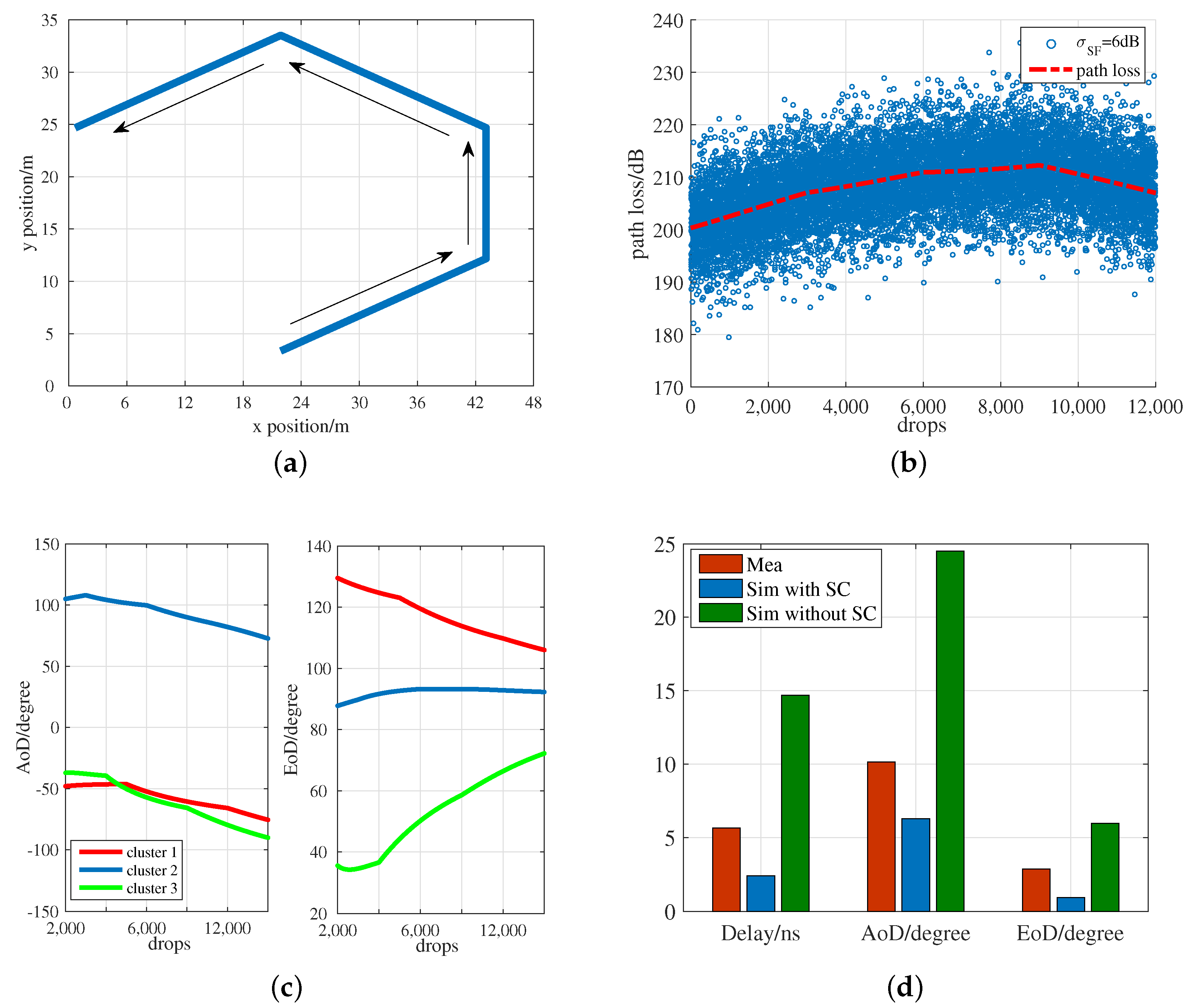
3.2. Simulation Results

A single-cell MIMO system was assumed at 3.5 GHz with 200 MHz bandwidth in a UMa NLoS scenario. At the Tx side, a UPA with 128 cross-polarized antennas was used; at the Rx side, a single-antenna ODA was used. Channel realizations in simulations were based on 12,000 drops. It is noted that the number of antennas is 1 on the Rx side since only the angles at the departure side could be observed. Moreover, the multiantenna array used at the Rx side in our measurement can be seen as an equivalent single antenna with an omnidirectional antenna pattern.
The MS moving trajectory is shown in Figure 7a. The Rx moves along in the direction of the arrow. Each direction takes 3000 drops. Based on Tx and Rx locations and the setting scenario, the path loss model is plotted in Figure 7b. The slope of the path loss model changes with the turning of directions. Blue bubbles show corresponding shadowing fading σ S F = 6 dB. Figure 7c shows the AoD and EoD evolution profiles of the first three clusters (with the three largest powers). Cluster angles change direction when the moving route changes, and the evolution process turns smoothly and continuously. We also calculated the standard deviations (STD) of the delay, and the AoD and EoD from the measurements and simulations with and without the spatial-consistency feature (see Figure 7d). The simulation group without the spatial-consistency feature always has the largest values. Compared to the STD from the simulation group without this feature, the simulation group with it gets closer to the measurement group, which implies that spatial consistency improves simulation performance.

4. Gradient Boosted Decision Tree-Based Model

4.1. Model Description

Generally, a decision-tree algorithm can be drawn as a flowchart that is easy to read and understand, and it can mainly be divided into two kinds: classification tree and regression tree. Boosting algorithms are a family of algorithms that can promote weak learners to strong learners. The gradient boosting machine (GBM) can use different learning methods than basic learners. GBDT is a GBM that uses the decision tree as the basic learner. It is a machine learning algorithm that is used for regression issues, originated and developed by L. Breiman and J. H. Friedman [25,26,27]. It is an ensemble learning method that is used to explain and predict statistical models, and it is flexible enough to fit different types of data, such as nonlinearities and interactions [28]. It sets each feature in each leaf node for stating the different characteristics of the dataset, and it goes through all child datasets to build the tree for predicting. In contrast to other decision-tree algorithms, GBDT reduces the residual in each training iteration by compared to previous training results. It creates a new mathematical model in each iteration to lower the residual. There, it can better lower the possibility of overfitting that another decision tree has [29].
GBDT can be seen as an addictive model F ( x ; w ) that is accumulated by T trees
F ( x ; w ) = t = 0 T α t h t ( x ; w ) = t = 0 T f t ( x ; w t )
where x are the input samples and w are the splitting variables, h is the regression-tree function, and α is the weight of each tree.
Optimized model F * can be obtained by minimizing loss function L ( · )
F * = arg min F i = 0 N L ( y i , F ( x i ; w ) )
where y i represents the ith output from the model.
According to the first-order Taylor expansion, the best steepest-descent step direction y i can be calculated as
y i ˜ = [ L ( y i , F ( x i ) ) F ( x i ) ] F ( x ) = F t 1 ( x )
Optimized solution w * can be obtained from
w * = arg min w , β i = 1 N ( y i ˜ β h t ( x i ; w ) ) 2
Then, we can obtain optimized line search ρ * by
ρ * = arg min ρ i = 0 N L ( y i , F t 1 ( x i ) + ρ h t ( x i ; w * ) )
Finally, the approximation is updated by
f t = ρ * h t ( x ; w * ) F t = F t 1 + f t

4.2. Numerical Results

Simulation and measurement data were used to train and validate the GBDT-based model. 80 % of the data are training samples, and 20 % are validating samples. Training samples are used to train the model, and validating samples are used to check its accuracy. To train the simulation data, we had to reconstruct CIRs in the time domain with MPC delay and power as input. Training output is the cluster delay, AoD, and EoD. To train the data collected by measurement, CIRs are ready-made as input, and the output is from the results given by the KPMKF process, as shown in Section 2. The depth of trees was set as 100, and the maximum iteration is set as 200.
To validate the GBDT-based model, RMSE was used to measure the differences between predicted and observed values, which is calculated by
R = n = 1 N ( y ( n ) y s i m / m e a ( n ) ) 2 N
y ( n ) is the nth results predicted by the GBDT-based model, while y s i m / m e a ( n ) is the nth results from simulations/measurements. N is the number of drops. The smaller the RMSE is, the better the fit between the predicted and observed values is.
Figure 8a displays an example of AoD results by GBDT to show the degree of fitting. The training and validating samples, and the AoDs of the three clusters, are from the above Section 3 simulation in NLoS conditions, which are shown as solid curves. The dotted lines are the fitted results calculated by the GBDT-based model. The fitted curves are very close to the samples.
The RMSEs of the measurements and simulations are shown in Figure 8b. This shows that the GBDT validating results generally fit well with simulation/measurement results. Compared to the measurement RMSEs, those of the simulations are smaller. Moreover, the GBDT-based model performs better in an LoS condition than in an NLoS condition.

5. Conclusions

In this paper, a series of cluster analyses of mobile UMa channels are presented, which were based on measurements and simulations. A UMa massive MIMO pedestrian mobile measurement at 3.5 GHz, which was performed with a virtual-measurement method, was described and analyzed. With the KPMKF algorithm for clustering and tracking, the spatial distributions of clusters in LoS and NLoS conditions were shown, respectively. From the figures, we could observe the cluster birth and death process and their spatial evolution during movement. The cluster birth and death histogram per snapshot was shown. The total snapshots of newly appeared clusters per snapshot was slightly larger than that of newly disappeared clusters per snapshot. The change of one or two clusters per snapshot takes more probabilities. In addition, the CDF of lifetime distances and VR diameters in Reference [9] were shown. In an LoS condition, most clusters showed shorter lifetime distances, which were less than 1 m.
To get closer to the above channel conditions, channel simulations were implemented with the IMT-2020 channel model using the newly introduced spatial-consistency feature. With the simulation results, the evolution of generated clusters could be observed. They evolve smoothly when UT turns the direction. Additionally, comparisons between measurements and simulations with and without this feature were given by STD. The results showed that simulation with this feature was closer to the measured channels.
The GBDT-based model, which is used for training and validating the above results from measurements and simulations, was introduced. We used the RMSE to check the accuracy of the model. Compared to the measurements, simulation RMSEs were smaller. Additionally, the GBDT-based model had better performance in an LoS condition than in an NLoS condition. Generally, it is a promising model for characterizing cluster evolution in linear mobile scenarios.

Author Contributions

Conceptualization, C.W. and J.Z.; methodology, C.W. and J.Z.; software, C.W. and G.Y.; validation, C.W., J.Z., and G.Y.; formal analysis, C.W. and J.Z.; investigation, C.W. and J.Z.; resources, C.W. and J.Z.; data curation, C.W. and J.Z.; writing—original draft preparation, C.W.; writing—review and editing, C.W., J.Z., and G.Y.; visualization, C.W.; supervision, J.Z.; project administration, J.Z.; funding acquisition, J.Z.

Funding

The research was supported by the National Science and Technology Major Project of the Ministry of Science and Technology (Grant No. 2018ZX03001031), the Key Program of the Beijing Municipal Natural Science Foundation (Grant No. L172030), and the project from the Beijing Municipal Science and Technology Commission (Grant No. Z181100003218007).

Acknowledgments

The authors thank Fredrik Tufvesson, Jose Flordelis, Huihui Ma, and Jian Zhang for active discussions.

Conflicts of Interest

The authors declare no conflict of interest.

References

  1. ITU M. 1225: Guidelines for Evaluation of Radio Transmission Technologies For IMT-2000. Report ITU 1997.
  2. ITU M. 2135: Guidelines for Evaluation of Radio Interface Technologies for IMT-Advanced. Report ITU 2009.
  3. ITU M. 2412: Guidelines for Evaluation of Radio Interface Technologies for IMT-2020. Report ITU 2017.
  4. Czink, N.; Yin, X.; Ozcelik, H.; Herdin, M.; Bonek, E.; Fleury, B.H. Cluster Characteristics in a MIMO Indoor Propagation Environment. IEEE Trans. Wirel. Commun. 2007, 6, 1465–1475. [Google Scholar] [CrossRef]
  5. Hentila, L.; Alatossava, M.; Czink, N.; Kyosti, P. Cluster-level Parameters at 5.25 GHz Indoor-to-Outdoor and Outdoor-to-Indoor MIMO Radio Channels. In Proceedings of the 2007 16th IST Mobile and Wireless Communications Summit, Budapest, Hungary, 1–5 July 2007; pp. 1–5. [Google Scholar]
  6. Poutanen, J.; Haneda, K.; Salmi, J.; Kolmonen, V.M.; Tufvesson, F.; Vainikainen, P. Analysis of Radio Wave Scattering Processes for Indoor MIMO Channel Models. In Proceedings of the 2009 IEEE 20th International Symposium on Personal, Indoor and Mobile Radio Communications, Tokyo, Japan, 13–16 September 2009; pp. 102–106. [Google Scholar]
  7. Poutanen, J.; Haneda, K.; Salmi, J.; Kolmonen, V.M.; Vainikainen, P. Modeling the Evolution of Number of Clusters in Indoor Environments. In Proceedings of the 2010 Fourth European Conference on Antennas and Propagation (EuCAP), Barcelona, Spain, 12–16 April 2010; pp. 1–5. [Google Scholar]
  8. Huang, C.; He, R.; Zhong, Z.; Geng, Y.; Li, Q.; Zhong, Z. A Novel Tracking-Based Multipath Component Clustering Algorithm. IEEE Antennas Wirel. Propag. Lett. 2017, 16, 2679–2683. [Google Scholar] [CrossRef]
  9. Wang, C.; Zhang, J.; Tian, L.; Liu, M.; Wu, Y. The Spatial Evolution of Clusters in Massive MIMO Mobile Measurement at 3.5 GHz. In Proceedings of the 2017 IEEE 85th Vehicular Technology Conference (VTC Spring), Sydney, Australia, 4–7 June 2017; pp. 1–6. [Google Scholar]
  10. Wang, C.; Zhang, J.; Tian, L.; Liu, M.; Wu, Y. The Variation of Clusters with Increasing Number of Antennas by Virtual Measurement. In Proceedings of the 2017 11th European Conference on Antennas and Propagation (EUCAP), Paris, France, 19–24 March 2017; pp. 648–652. [Google Scholar]
  11. Zhang, J. The Interdisciplinary Research of Big Data and Wireless Channel: A Cluster-nuclei Based Channel Model. China Commun. 2016, 13, 14–26. [Google Scholar] [CrossRef]
  12. Gao, J.; Zhang, J.; Xiong, Y.; Sun, Y.; Tao, X. Performance Evaluation of Closed-loop Spatial Multiplexing Codebook based on Indoor MIMO Channel Measurement. Int. J. Antennas Propag. 2012, 2012, 701985. [Google Scholar] [CrossRef]
  13. Zhang, J.; Pan, C. Validation of Antenna Modeling Methodology in IMT-Advanced Channel Model. Int. J. Antennas Propag. 2012, 2012. [Google Scholar] [CrossRef]
  14. Liu, M.; Zhang, J.; Zhang, P. Outage Probability of Dual-hop Multiple Antenna Relay Systems with Interference at the Relay and Destination. Int. J. Antennas Propag. 2014, 13, 2308–2321. [Google Scholar] [CrossRef]
  15. Yu, H.; Zhang, J.; Zheng, Q.; Zheng, Z.; Tian, L.; Wu, Y. The Rationality Analysis of Massive MIMO Virtual Measurement at 3.5 GHz. In Proceedings of the 2016 IEEE/CIC International Conference on Communications in China (ICCC Workshops), Beijing, China, 16–18 August 2016; pp. 1–5. [Google Scholar] [CrossRef]
  16. Fleury, B.H.; Tschudin, M.; Heddergott, R.; Dahlhaus, D.; Pedersen, K.I. Channel Parameter Estimation in Mobile Radio Environments using the SAGE Algorithm. IEEE J. Sel. Areas Commun. 1999, 17, 434–450. [Google Scholar] [CrossRef]
  17. Sengijpta, S.K. Fundamentals of Statistical Signal Processing: Estimation Theory; Prentice Hall: Upper Saddle River, NJ, USA, 1995. [Google Scholar]
  18. Czink, N.; Tian, R.; Wyne, S.; Eriksson, G.; Tufvesson, F.; Zemen, T.; Nuutinen, J.; Ylitalo, J.; Bonek, E.; Molisch, A. Tracking Time-variant Cluster Parameters in MIMO Channel Measurements: Algorithm and Results. In Proceedings of the International Conference on Communications and Networking in China (ChinaCOM), Shanghai, China, 22–24 August 2007. [Google Scholar]
  19. Czink, N.; Cera, P.; Salo, J.; Bonek, E.; Nuutinen, J.; Ylitalo, J. A Framework for Automatic Clustering of Parametric MIMO Channel Data Including Path Powers. In Proceedings of the IEEE Vehicular Technology Conference, Melbourne, Australia, 7–10 May 2006; pp. 1–5. [Google Scholar]
  20. Liu, L.; Oestges, C.; Poutanen, J.; Haneda, K.; Vainikainen, P.; Quitin, F.; Tufvesson, F.; Doncker, P.D. The COST 2100 MIMO Channel Model. IEEE Wirel. Commun. 2012, 19, 92–99. [Google Scholar] [CrossRef]
  21. 3GPP TR 38.900 V14.2.0 Technical Report: Study on Channel Model for Frequency Spectrum above 6 GHz (Release 14) 2016. Available online: http://www.3gpp.org/ (accessed on 26 February 2019).
  22. 3GPP TR 36.873 V12.4.0 Technical Report: Study on 3D Channel Model for LTE (release 12) 2017. Available online: http://www.3gpp.org/ (accessed on 26 February 2019).
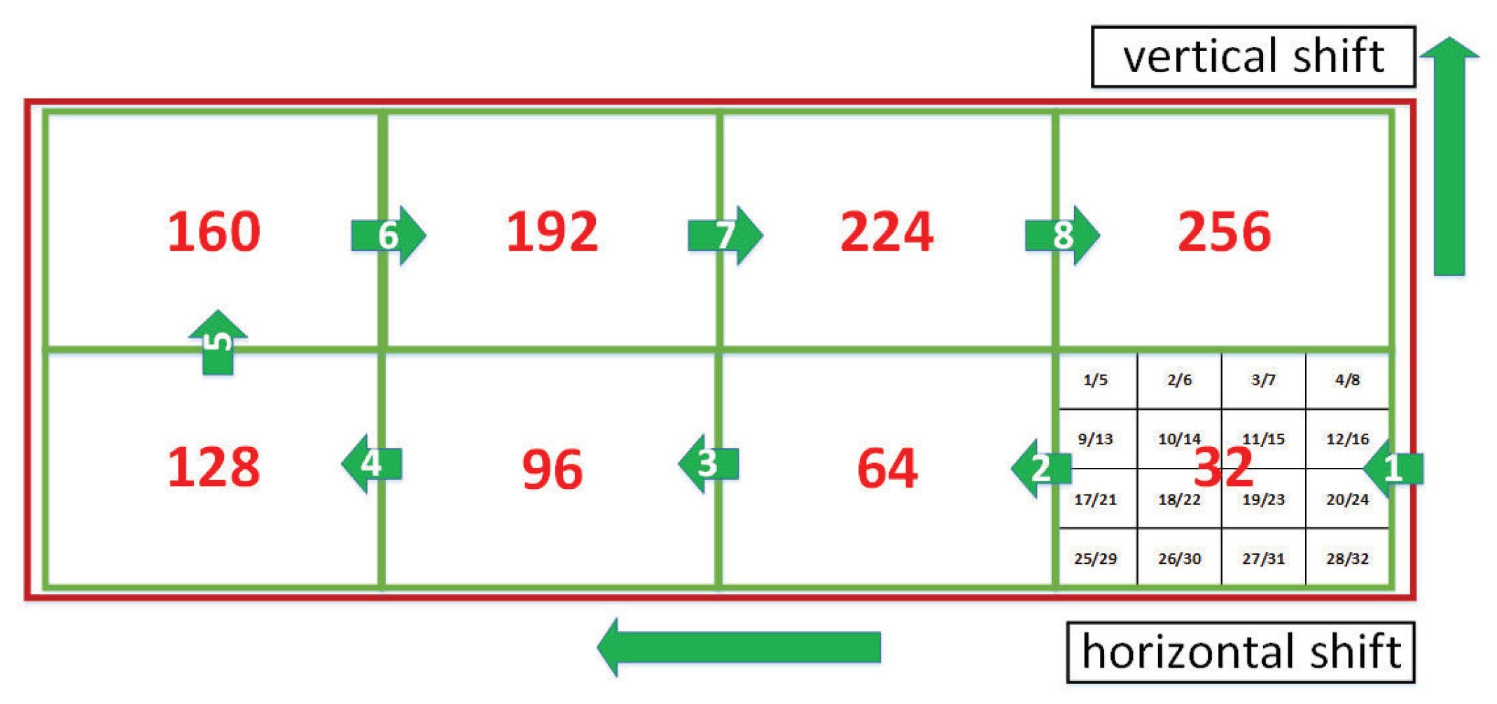
  23. Zhang, J.; Zheng, Z.; Zhang, Y.; Xi, J.; Zhao, X.; Gui, G. 3D MIMO for 5G NR: Several Observations from 32 to Massive 256 Antennas Based on Channel Measurement. IEEE Commun. Mag. 2018, 56, 62–70. [Google Scholar] [CrossRef]
  24. Yang, M.; Zhang, S.; Shao, X.; Guo, Q.; Tang, W. Statistical Modeling of the High Altitude Platform Dual-polarized MIMO Propagation Channel. China Commun. 2017, 14, 43–54. [Google Scholar] [CrossRef]
  25. Friedman, J.H. Greedy Function Approximation: A Gradient Boosting Machine. Ann. Stat. 2001, 29, 1189–1232. [Google Scholar] [CrossRef]
  26. Breiman, L. Arcing the Edge; Technical Report, Technical Report 486; Statistics Department, University of California at Berkeley: Berkeley, CA, USA, 1997. [Google Scholar]
  27. Friedman, J.H. Stochastic Gradient Boosting. Comput. Stat. Data Anal. 2002, 38, 367–378. [Google Scholar] [CrossRef]
  28. Elith, J.; Leathwick, J.R.; Hastie, T. A Working Guide to Boosted Regression Trees. J. Anim. Ecol. 2008, 77, 802–813. [Google Scholar] [CrossRef] [PubMed]
  29. Vezhnevets, A.; Barinova, O. Avoiding Boosting Overfitting by Removing Confusing Samples. In Proceedings of the European Conference on Machine Learning, Warsaw, Poland, 17–21 September 2007; Springer: Berlin, Germany, 2007; pp. 430–441. [Google Scholar]
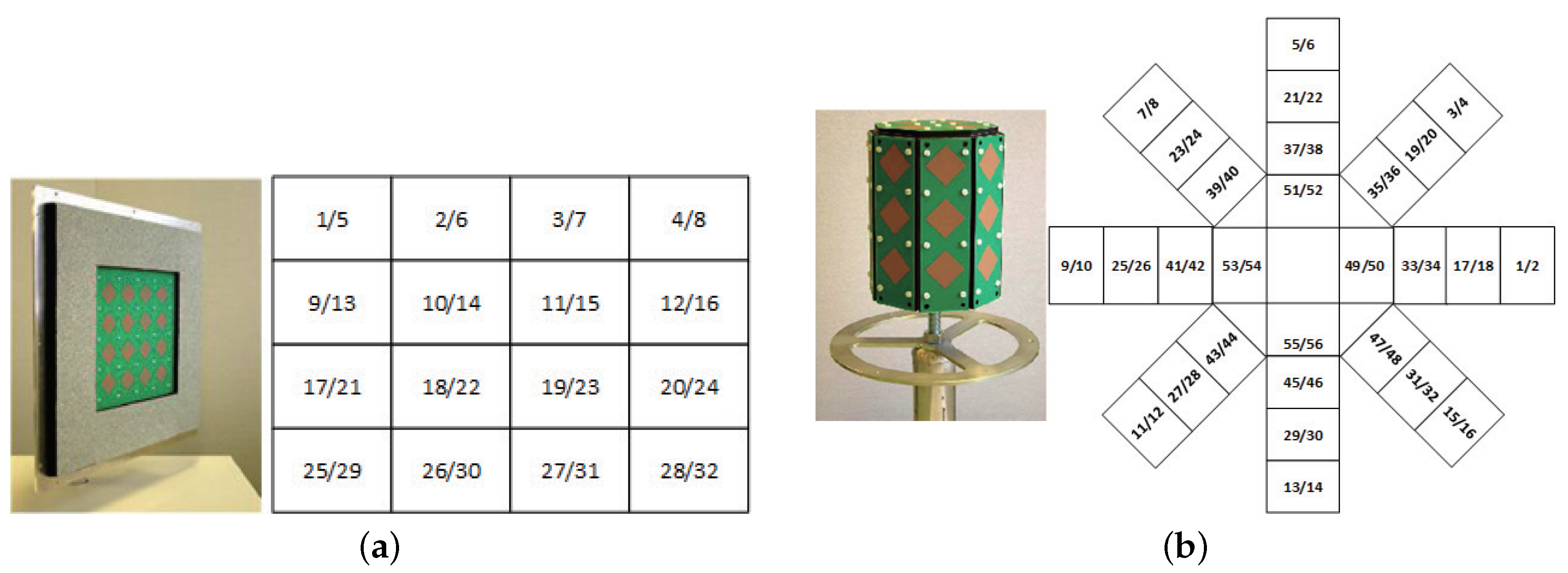
Figure 1. Measurement map (Red triangle is the Tx location. R1 and R2 are the measurement routes in LoS and NLoS conditions, respectively).
Applsci 09 00886 g001
Figure 2. Antenna used in the measurement. (a) Tx: 4 × 4 patches, with each patch comprising a pair of cross-polarized antennas. (b) Rx: 8 adjacent sides with 3 patches each, a top surface with 4 patches; each patch contains a pair of cross-polarized antennas.
Applsci 09 00886 g002
Figure 3. Scheme of antenna combining array in virtual measurements.
Applsci 09 00886 g003
Figure 4. Flowchart of the K-power means-Kalman filter (KPMKF) algorithm.
Applsci 09 00886 g004
Figure 5. Clustering and tracking profiles of measurement clusters. (a) Cluster-tracking profiles in LoS condition. (b) Cluster-tracking profiles in NLoS condition. (c) Birth and death histogram of clusters per snapshot. (d) cumulative density functions (CDF) of cluster lifetime distances (m).
Applsci 09 00886 g005
Figure 6. Framework of primary module in IMT-2020 channel model.
Applsci 09 00886 g006
Figure 7. Profiles of the IMT-2020 channel simulations in UMa, 3.5 GHz, and STD comparisons among measurements and simulations with and without spatial-consistency feature. Note: AoD, azimuth angle of departure; EoD, elevation angle of departure; STD, standard deviation. (a) MS moving trajectory. (b) Simulation path loss model. (c) AoD and EoD of first three clusters (three largest powers). (d) Delay STD, AoD, and EoD.
Applsci 09 00886 g007
Figure 8. Profiles of GBDT-based model. (a) AoD example of degree of fitting. (b) RMSE.
Applsci 09 00886 g008
Table 1. Specifications of measurement campaign.
Antenna TypeODA(Rx)UPA(Tx)
Number of antenna ports56 (16 ports were used)32
Radiation patternOmnidirectionalHemispherical
Inter element spacing41 mm41 mm
Number of elements2816
Polarized ± 45 ± 45
Angle rangeAzimuth 180 180 70 70
Elevation 70 90 70 ∼70
Center frequency3.5 GHz
Bandwidth200 MHz
PN sequence255 chips
Speed of Rx1.4 m/s (pedestrian)

