A State-Space Analysis of a Single Zone Building Considering Solar Radiation, Internal Radiation, and PCM Effects

Abstract

This paper deals with the dynamic modeling of a typical single-zone building. It describes the development of a dynamic model for thermal transient analysis and its application to a simplified test case considering solar irradiation and internal radiation. The dynamic behavior of the indoor air temperature has been investigated by means of a lumped approach using a state-space representation developed in MATLAB/Simulink. A set of daily temperature profiles, which are representative of the Mediterranean climatic condition, on a few different winter days, has been used as boundary conditions for the dynamic simulations. In addition, the model has been validated using two different sets of experimental data available in the literature, both statically and dynamically. Finally, a layer of insulation with a phase change material (PCM) is applied to the single zone building to quantify its effect on the building’s behavior. The results showed that the rate and amount of energy consumption in the building with PCM are moderately lower than the building without PCM. In addition, the variation of inlet air temperature, solar effects, and energy consumption have been evaluated for a case study example, as well as comfort in transient simulation to achieve a complete evaluation of the test building investigated. A satisfactory agreement was obtained between the experimental and the simulation results and shows that the model can be used for a wide range of materials, dimensions, thermal resistances, and boundary conditions.

1. Introduction

Over the past ten years, the study of building energy consumption has been a significant topic of investigation [1,2,3,4,5,6,7,8,9,10,11,12]. According to International Energy Agency information, more than 32% of energy is used in residential and commercial sectors, and about 40% of this energy is applied for the space heating [13]. Most European countries have a temperate climate in summer and are major energy consumers during the winter [12,14].

Even in moderate climate regions, like Genoa, the outdoor temperature is lower than 15 °C for more than 46% of the year [15], and this fact corresponds to a large consumption of energy for heating of civil, commercial, and industrial buildings. For this reason, governments adopt policies of incentives and taxes in order to encourage people to renew and enhance the energy efficiency of their buildings, and to pay special attention to the retrofitting of old and historical ones [15,16]. The heat demand in residential buildings depends on various factors, such as the number of inhabitants, the outdoor temperature, and the number of wall layers, the wall thickness, and the insulation. Considering the changes of all the factors mentioned above during the day, and also during the year, it is understandable that the thermal analysis of buildings, in order to be accurate, requires a dynamic and unsteady modelization [16,17,18,19,20].

Several studies have been carried out in the field of heat transfer modeling in buildings and in the prediction of inside temperature. Athientis et al. [21] performed a centralized approach to building’s thermal control and energy analysis. In addition, Laplace transfer functions for the building were obtained by means of thermal network models, HVAC systems, and control components. The results showed a separation of building’s thermal dynamics into short-term and long-term dynamics for convective loads. Additionally, air temperature sensor time constants were shown to have a strong effect on room temperature response to set point changes, such as an increase of 50% in the settling time when the sensor time constant was increased from 30 s to 60 s [21].

In recent years, due to the importance of energy conservation, the high cost and time required for experimental studies, and the rapid evolution of computer performance and techniques, the development of numerical methods aimed at solving this kind of problem have greatly increased. In particular, several mathematical models have been developed in order to simulate the thermal behavior of buildings within the MATLAB/Simulink environment [11,22,23,24].

Hudson et al. developed a computationally efficient thermal model of a simple building by using Simulink: Here, the building was described by means of the electric analogy model; the system of thermal resistance and capacities was represented by the RC circuit problem. They used a high-mass building with one layer of walls. Additionally, the model was tested using experimental data from a building with high thermal capacity [25].

Mendes et al. derived the energy balancing equations in a transient condition using CFD and Simulink. A lumped approach was used for the model of room air temperature and a multi-layer model for the building envelope. The results were evaluated with a controllable weather condition test room. Comparison between the theoretical and calculated data showed a notable agreement [26].

Ramos et al. implemented a numerical model using MATLAB/Simulink. This work also illustrated the moisture buffer capacity of building materials in transient conditions: Numerical simulation for hygro-thermal performance and experimental data were compared showing good agreement [27].

Kalagasidis et al. developed a software package for heating, HVAC, and moisture system analysis in buildings. The toolbox was constructed as a modular structure of standard building elements, using the graphical programming language, Simulink. To enable development of the toolbox, a common modeling platform was defined: A set of unique communication signals, material database, and documentation protocol [28].

Kulkarni et al. showed a proportional control system for residential buildings by setting up a dynamic simulation including the control system. An optimized MATLAB state-space method was used to model the heating system. Their results confirmed that proportional control was preferable to the two-position control for the thermal comfort, while there was not much difference in energy consumption between the two control systems [29].

Marsik et al. presented a dynamic model for evaluating energy consumption associated with ventilation. In addition, the model was used to study three ventilation scenarios of a typical home in Fairbanks—natural ventilation, a heat recovery ventilator (HRV), and an HRV with an additional particulate filter. The results highlighted a significant reduction of annual costs for energy [30].

Gamberi et al. developed an innovative method for modeling multi-zone hydronic heating systems in buildings, again using the MATLAB/Simulink environment. A laboratory heating system was used for validation of the model. A series of trials were conducted in a multi-zone laboratory heating system located within the R&D division of a leading Italian boiler manufacturer [31].

Chen et al. presented a Simulink model for simulating principles of a dynamic HVAC component model. The simulation result demonstrated that schedule-based temperature and damper position reset has a significant influence on energy conservation for summer and winter. Their simulation program can be particularly useful for dynamic analysis of different HVAC control strategies [32].

Borelli et al. developed a dynamic model of a building heating plant. The model, validated by means of experimental data collected by monitoring a real Italian building, showed very good agreement between measured and calculated data, and was used to assess different scenarios regarding the revamping of the heating plant [33].

Mankibi et al. modeled the thermal behaviors of a multi-layer living wall. The aim of this study was to identify the most efficient wall configuration according to indoor and outdoor climate conditions by using a new simulation tool developed using MATLAB/Simulink. Furthermore, phase change materials were implemented in this research. The results showed an optimized active multi-layer living wall system could allow 27%–38% of reduced heating energy consumption while avoiding thermal discomfort [34].

Sasic Kalagasidis generated a numerical model of a building with PCM to obtain the energy usage for heating and cooling of buildings. The model was validated by experimental measurements and a normative benchmark of a whole building. The author used the international building physics toolbox for her simulation and the results showed that the annual saving of total energy for heating and cooling was varied between 5% to 21% depending on the thermal comfort and the PCM position through the building [35].

Much of the research previously described used only solar effects or only internal radiation. Nevertheless, both these aspects have a significant effect on energy consumption. For this reason, models considering both lead to more accurate results.

The paper is articulated as follows: A general recall of the rules for energy saving in Genoa (Italy); a description of the mathematical model; a description of the experimental facilities used to validate the model; validation of the model with available experimental results; and finally utilization of the validated model to analyze two different case studies.

The mathematical model for predicting the building thermal behavior takes into account solar radiation, internal radiation, presence of furniture, occupancy, and lighting. The model is then used to simulate a simple building with multi-layer walls in a residential area of Genoa, Italy, using real meteorological data as input. Several different set points are also investigated, showing that they have a relevant effect on the net energy consumption and on the impact of building thermal mass. The energy balance equations are solved for each surface such as roof, floor, and interior and exterior walls, separately. The model calculates the internal conditions of the building using the energy balance equations for walls and internal materials. The system of partial differential equations, in space and time, has been written in the form of a state-space matrix and solved using MATLAB/Simulink. In addition, a layer of PCM insulation is later applied in the model and its behavior discussed.

This method has high efficiency in terms of computational and dynamic responses, since they do not have a high computational cost and the computational times are low. This model estimates the variations of each layer temperature of the walls, generated by the continuous changes of the external temperature.

2. Main Rules for Energy Saving in Genoa

The inventory of buildings, located in Genoa, slightly exceed 33,000 items (2001 census [36]), most of which were built between the 1920s and 1970s; about 89% are residential buildings, resulting in around 300,000 homes and apartments. About 68% of the existing buildings are occupied and about half of them have central heating for all the apartments.

A rough estimation of actual overall specific heat consumption for heating Genoese buildings (estimated considering start–stop operating regime), amounts to 151 kWh/m² per year, which must be compared to the legally prescribed mean requirement value (Legislative Decree no. 192/2005) of 40 kWh/m² per year, for new buildings. The net discrepancy is because of lack of regulations at the time in which most of the buildings were built. This is also combined with the tendency, especially in the last three decades of the 20th century, to build blocks in which each apartment has its own independent heating system, resulting in low efficiency and high consumption.

Recent rules transpose the EU directives about energy consumption of residential and industrial buildings have triggered private investments aimed at energy savings. Despite that, at the same time there has been an increase in energy consumption due to the growing demand for air conditioning and other cooling systems during summer months [37].

3. Mathematical Model

In this section, the mathematical equations for dynamic conditions, are duly described, together with the corresponding boundary conditions.

3.1. Definition of the Problem

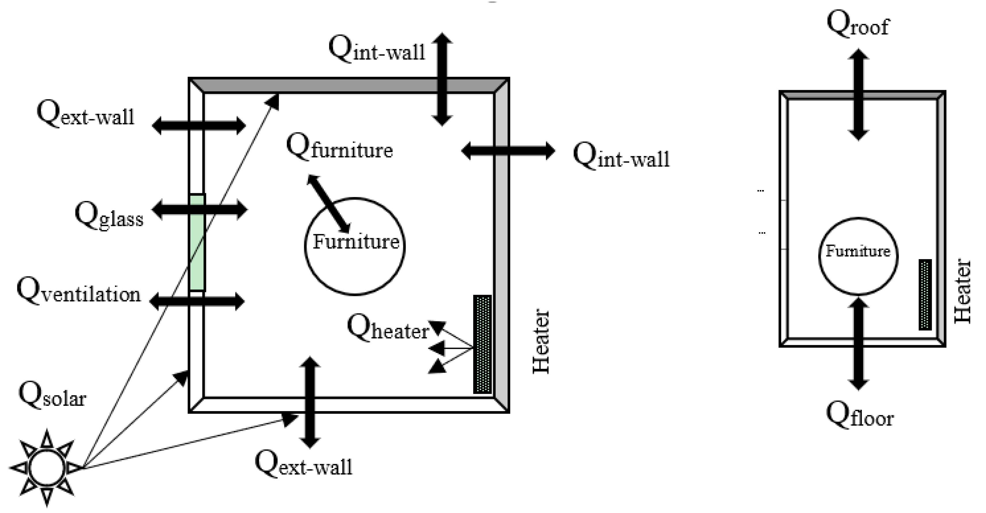
Conduction, convection, and radiation are the processes involved in heat transfer through the building’s envelope. Heaters and the solar radiation through windows are considered as heat gains within the building, namely solar gain and heaters.

The model takes into consideration thermal resistances and thermal capacities of wall, windows and furniture, solar radiation and radiation between internal surfaces, ventilation, and heat generated by appliances. The effects of solar radiation have been considered both for the direct and instantaneous increase of effective temperature of the outer surfaces of external walls and for the heat gain corresponding to the part, which is transmitted through the windows, and which is located at the internal surfaces. Finally, radiative heat transfer among surfaces has been calculated: Walls, floor, roof, heater, and furniture have been considered as diffuse grey surfaces, and the matrix of the view factors, of each surface to any other one, has been evaluated.

Figure 1 shows the sources and the sinks of energy through a typical building, such as the one considered in this study.

For the inlet air in the single zone building, the balancing of the energy equation is derived by:

$$\begin{gathered} {\rho }_a{c}_a{v}_a\frac{d{T}_{inlet}}{dt}=Q_{ext-wall}+Q_{int-wall}+Q_{roof}+Q_{floor}+Q_{furniture}+Q_{heater} \\ +Q_{glass}+Q_{ventilation}+Q_{gen}={\displaystyle \sum }_i^{}{Q}_i+Q_{gen} \end{gathered}$$

(1)

where Q_i is the rate of heat transfer for the exterior and internal walls, roof, floor, ventilation, windows, and furniture. Additionally, Q_gen is the rate of thermal generation due to the building’s indoor equipment.

3.2. Definition of the General Model of the Wall

Fundamentally, the thermal analysis of a wall should be developed dynamically, because the heat transfer through the wall is dependent on time and place. There are several different methods to analyze a building’s envelope. According to the one-dimensional Fourier equation:

$$\frac{{\partial }^{2}T}{\partial x^2}=\frac{1}{\alpha }\frac{\partial T}{\partial \tau }$$

(2)

where α is the thermal diffusivity coefficient of the medium, [m²/s], given by α = λ/(c_p ρ).

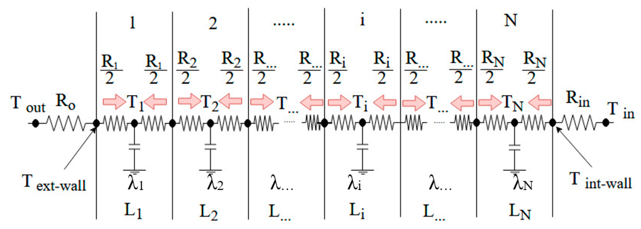
Equation (2) is solved by means of numerical techniques such as FEM (as well as analytically for small systems). Another way of solving Equation (2) is to transfer the PDE Fourier model to the ordinary differential equations (ODEs). The used lumped capacitance model is an ODE model and assumes that the temperature difference inside each lump is negligible. In this way, the wall is divided into some individual elements or lumps, in which the temperature is considered constant and independent of time.

Figure 2 shows the layout of an external wall with the thermal resistance model [11]. External walls are notable nodes in the building envelope because these are consequently affected by solar and internal irradiation. The effect of solar radiation is accounted by means of the increase of temperature which it induces on the external surface of the wall.

The energy balance equation for the nodes of wall, roof, and floor can be written as follows:

For the first node (i.e., T₁), the energy balance equation is:

$$\begin{gathered} M_1{c}_{v1}\frac{d{T}_1}{dt}\text{=}{U}_{o,1}A\left(T_{eq}-T_1\right)-U_{1,2}A\left(T_1-T_2\right) \\ {U}_{o,1}=\frac{1}{\frac{1}{h_o}+\frac{L_1}{2{\lambda }_1}} , U_{1,2}=\frac{1}{\frac{L_1}{2{\lambda }_1}+\frac{L_2}{2{\lambda }_2}} \end{gathered}$$

(3)

where M₁, c_v1, and T₁ are mass, specific heat, and the temperature of layer 1, respectively. U_o,1 and U_1,2 are overall heat transfer coefficients, and A and R are the wall area and thermal resistance, respectively. In addition, L₁, L₂ are the thicknesses and λ₁, λ₂ are the thermal conductivity of the first and second layer.

For the exterior wall, the equivalent temperature (T_eq) is calculated instead of the outdoor temperature, because solar irradiation has direct effects on the outside surface temperature and depends on the location of the sun’s azimuth and elevation during the day.

$$T_{eq}=T_{out}+\frac{{\epsilon }_{ext}I}{h_o}$$

(4)

where T_out, ε_ext, I, and h_o are the outside temperature, the absorptivity, the total solar irradiation according to the geographical position [12], and the outside convective heat transfer coefficient, respectively.

For the internal nodes, number 2 to N-1:

$$\begin{array}{c}{M}_i{c}_{vi}\frac{d{T}_i}{dt}\text{=}{U}_{i-1,i}A\left(T_{i-1}-T_i\right)-U_{i,i+1}A\left(T_i-T_{i+1}\right)\\ U_{i-1,i}=\frac{2}{R_{i-1}+R_i}\\ U_{i,i+1}=\frac{1}{\frac{L_i}{2{\lambda }_i}+\frac{L_{i+1}}{2{\lambda }_{i+1}}}, U_{i-1,i}=\frac{1}{\frac{L_{i-1}}{2{\lambda }_{i-1}}+\frac{L_i}{2{\lambda }_i}} \end{array}$$

(5)

where M_i, c_vi, T_i, and R_i are the mass, the specific heat, the temperature, and thermal resistance of ith layer, respectively. In addition, L_i is the thicknesses and λ_i is the thermal conductivity of the i^th layer.

Equation (6) describes the balance of energy for the last node N. Internal radiation plays vital roles in internal temperature on the in-surface node, heater, furniture, human, and everything that might be in the building.

$$\begin{gathered} \begin{array}{cc}{M}_N{c}_{vN}\frac{d{T}_N}{dt}=& U_{N-1,N}A\left(T_{N-1}-T_N\right)-U_{N,N}A\left(T_N-T_{in}\right) +\\ & -\sigma {\epsilon }_{int,h}{A}_h{F}_{s,h-N}\left[T_{w,N}^4\left(t\right)-T_h^4\left(t\right)\right]+\\ & -\sigma {\epsilon }_{int,N}{A}_N{\displaystyle \sum }{F}_{s,j-N}\left[T_{w,N}^4\left(t\right)-T_{w,j}^4\left(t\right)\right]\end{array} \\ {U}_{N,N}=\frac{1}{\frac{1}{h_{in}}+\frac{L_N}{2{\lambda }_N}}, U_{N-1,N}=\frac{1}{\frac{L_{N-1}}{2{\lambda }_{N-1}}+\frac{L_N}{2{\lambda }_N}} \end{gathered}$$

(6)

where, σ, ε_int,N, A, and F_s,j-N are the Stefan–Boltzmann constant, the N-layer emissivity, the surface area and the shape factor (radiation effect between two surfaces) of each surface on the other surfaces, respectively.

The energy balance equation for the heater can be written as follows:

$$\begin{gathered} M_h{c}_{vh}\frac{d{T}_h}{dt}=Q_{heater}-U_h\left(T_{in}-T_h\right)-\sigma {\epsilon }_{int,h}{A}_h{\displaystyle \sum }{F}_{s, h-N}\left[T_{w, N}^4\left(t\right)-T_h^4\left(t\right)\right] \\ {U}_h=A_h{h}_h \end{gathered}$$

(7)

where, ε_int,h, A_h, and F_s,h-N are the heater emissivity, the heater area, and the shape factor of the heater on the other surfaces, respectively, and Q_heater is the constant power of the heater.

The energy balance equation for the equipment and furniture can be written as follows:

$$\begin{gathered} M_f{c}_{vf}\frac{d{T}_f}{dt}=U_f\left(T_{in}-T_f\right)-\sigma {\epsilon }_{int,f}{A}_f{\displaystyle \sum }{F}_{s,f-N}\left[T_{w, N}^4\left(t\right)-T_f^4\left(t\right)\right] \\ {U}_f=\frac{1}{\frac{1}{A_f{h}_f}+\frac{L_f}{A_f{\lambda }_f}} \end{gathered}$$

(8)

where, ε_int,f, A_f, and F_s,f-N are the furniture emissivity, the furniture area, and the shape factor of the furniture on the other surfaces, respectively.

The energy balance equation for the windows are as follows:

$$\begin{gathered} M_w{c}_{vw}\frac{d{T}_w}{dt}=U_w\left(T_{in}-T_o\right)-\sigma {\epsilon }_{int,w}{A}_w{\displaystyle \sum }{F}_{s,w-N}\left[T_{w, N}^4\left(t\right)-T_w^4\left(t\right)\right] \\ {U}_w=\frac{1}{\frac{1}{A_w{h}_{in}}+\frac{L_w}{A_w{\lambda }_w}+\frac{1}{A_w{h}_o}} \end{gathered}$$

(9)

where, ε_int,w, A_w, and F_s,w-N are the windows emissivity, the windows area, and the shape factor of the windows on the other surfaces, respectively.

The energy balance equation for the ventilation can be written as follows:

$$\begin{gathered} M_v{c}_{vv}\frac{d{T}_v}{dt}=U_v\left(T_{in}-T_v\right) \\ {U}_v={\rho }_a{\dot{v}}_a{c}_a \end{gathered}$$

(10)

where, M_v, c_vv, and T_v are mass, specific heat, and the temperature of ventilation system, respectively. U_v is overall heat transfer coefficient and $\dot{v_a}$ is air volume of air-conditions to time.

In this study, a uniform distribution was assumed for the internal energy in the building in order to achieve an accurate simulation. The model was applied to a single zone building built in Genoa in 1980.

The set of differential equations, which describe the heat transfer through the different parts of the building, was obtained in the time-dependent form. By solving these equations, the changes of temperature were investigated in different components of the building. According to all above equations, there were 39 energy balance equations for the building (five for external east wall, five for external wall facing southward, six for internal wall, six for roof, six for floor, one for heater, one for internal air, one for internal equipment, and eight for the internal radiations).

Therefore, the obtained equations could be written in the state-space form as follows:

$$\begin{gathered} \dot{T}\left(t\right)=AT\left(t\right)+Bu\left(t\right) \\ y\left(t\right)=CT\left(t\right) \end{gathered}$$

(11)

where $\dot{T}$(t) and T(t) are the derivative temperature and physical temperature of each layer, respectively. Additionally, u(t) is a matrix related to the inputs, such as the boundary temperature condition on the wall surfaces and internal heat gains due to people’s activities, lighting, and other equipment. y(t) corresponds to the outputs, room, and layer temperatures.

The matrix elements of A and B contain the effects of physical properties and geometric characteristics of the system components on the temperature of different parts of the building [38].

$$\left[\begin{array}{c}\dot{T_1}\\ ⋮\\ \dot{T_{39}}\end{array}\right]=\left[\begin{array}{ccc}{A}_{1, 1}& \cdots & A_{1, 39}\\ ⋮& \ddots & ⋮\\ A_{39, 1}& \cdots & A_{39, 39}\end{array}\right]\times \left[\begin{array}{c}{T}_1\\ ⋮\\ T_{39}\end{array}\right]+\left[\begin{array}{ccc}{B}_{1, 1}& \cdots & B_{1, 39}\\ ⋮& \ddots & ⋮\\ B_{39, 1}& \cdots & B_{39, 39}\end{array}\right]\times \left[\begin{array}{c}{U}_1\\ ⋮\\ U_{39}\end{array}\right]$$

(12)

The state-space equations were solved by using the state-space functionalities integrated in the Simulink library. Outdoor temperatures, and east and south solar radiation for the first week of January were inputs for the state-space model. The variation of temperature for each layer, the inlet air temperature, and the energy consumption were the outputs of the state-space simulation.

4. Validation of the Model

The mathematical model was validated by comparing its results to experimental data, available in two experimental literature, as described below.

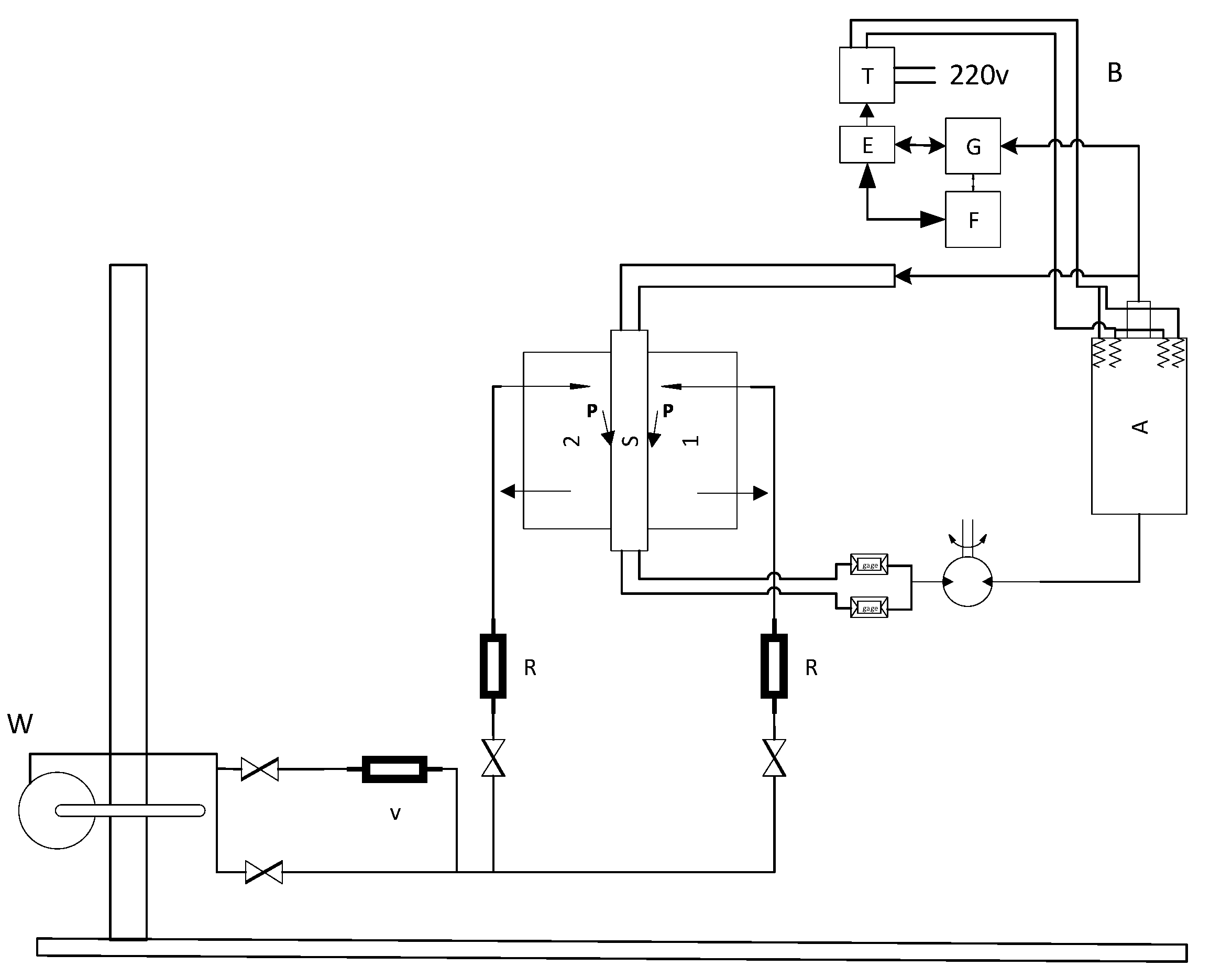
Milano, Reale, and Rubatto [39] developed an experimental set-up, designed to measure the periodic heat flow through the external walls of a room. The experimental equipment is shown schematically in Figure 3: The thermal source (S) consists of a steel prismatic container, inside of which water circulates. The temperature can be controlled, in time, according to a pre-established law, by means of the regulation system (B). The latter is made up of a boiler (A), in which the water is heated by an electrical resistance unit, the feeding of which is controlled by a transformer (T) through a regulation system (G), fed-back by the actual water temperature value at the entrance of the source (S). The temperature, measured at (S), is compared with the programmed value in (F) and adjusted by the regulator (E). The source (S) consists of a central zone, which is dedicated to the actual thermal transmission, and a guard ring, which prevents lateral leakages.

On both opposite sides of the source, the wall (P) being tested was fixed by means of appropriate fixing rods, in such a way as to achieve a symmetrical distribution of the thermal flux emitted from (S). The thermal capacity of the internal environment of the testing room was adjusted by means of 20 tubes of thin glass placed vertically, which contained water in different quantities according to the internal thermal capacity that one wishes to achieve.

Ventilation was provided feeding air into the two symmetric, insulated rooms (whose internal dimensions were 1.4 × 1.4 × 1.0 m, each). Air was extracted by a fan (W) from an external environment whose temperature was constant, in practice. In fact, the tests were carried out in a semi-basement laboratory with a volume of about 2,000 m³.

The volumetric flow of the ventilated air was measured by rotameters (R), whose calibration was controlled periodically by inserting a Venturi meter (V) into the circuit.

During the tests, measuring of the temperature was carried out by resistance thermometers, on the surface of the walls being tested, in contact with the source (S), and on the internal one facing of the environment delimited by the rooms (1 and 2), as well as on the inside of the rooms themselves.

The test panel was made of three layers and the specification of each one is shown in

Table 1. Test panel specifications [39].

Materials	L (m)	λ (w/m K)	C (kJ/kg K)	ρ (kg/m3)
Cement	0.0035	0.93	0.84	1900	Wall A
Polyurethane Foam	0.023	0.023	1. 3	40
Cement	0.0035	0.93	0.84	1900
Polystyrene Foam	0.1	0.032	1. 3	15	Wall B
Wood	0.02	0.11	2. 5	300
Glass Wool	0.06	0.058	0.8	75

.

The experimental tests were carried out realizing 30 determinations, each one lasting 5 days, imposing a sinusoidal thermal wave on the external face of the panel being tested and recording the form of the wave transmitted into the two rooms (1 and 2). During the tests, the amplitude of the sinusoidal wave imposed by the source S was equal to 16 ± 1 °C. The average temperature of the lab, in which the test section was placed, experienced a seasonal temperature excursion of about 10 °C and consequently, during the 150 days of tests, varied between 65 and 75 °C.

The various series of tests differed, one from another, for the different internal thermal capacity referred to the unit area of the walls being tested, named M, equal to 2, 15, and 25 [kJ/(m²K)], respectively. Finally, the air changes were made to vary from zero to 25 times the volume of the room, per hour.

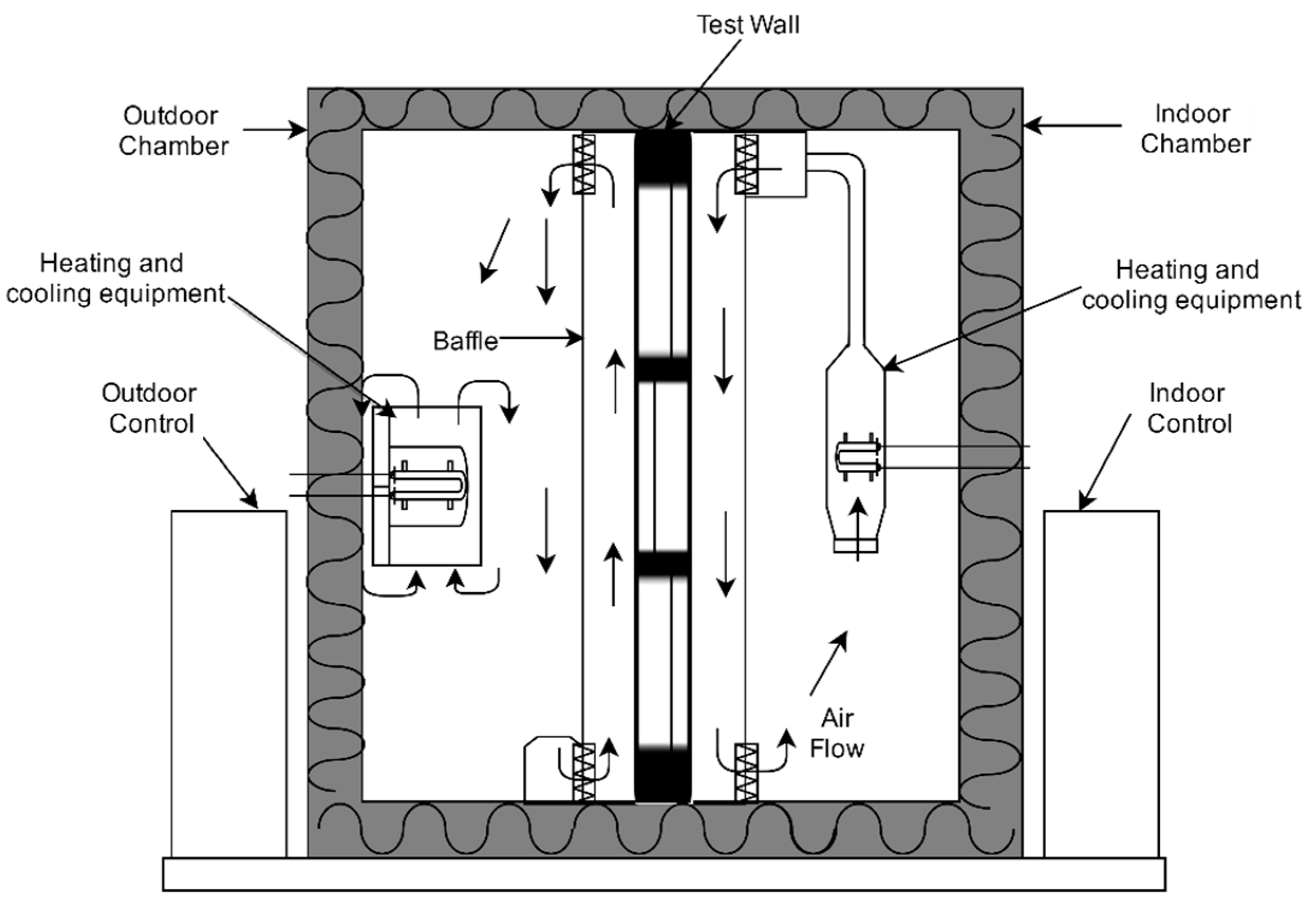
The second validation was based on the experiments by Fiorato and Cruz [40], in both steady-state and dynamic conditions, of six masonry walls, in order to investigate their heat transfer characteristics. The apparatus consisted of a calibrated hot box facility made up of two highly insulated chambers. This system was designed to accommodate walls with thermal resistances varying from 0.26 to 3.52 [K/(m²W)]. The outdoor chamber was maintained at a constant temperature or oscillating between −29 and 49 °C, and the indoor chamber was maintained between 18 and 27 °C [40]. The schematic of apparatus and wall characteristics is shown in Figure 4 and

Table 2. Wall characteristics [40].

Wall Configuration	Area (m2)	Layer Material	Thickness of Layers (m)	Density ρ (kg/m3) of Layers	Thermal Conductivity (W/m K) of Layers
1-Hollow block uninsulated	2.62 × 2.62	Concrete	0.203	1858	0.486
2-Hollow block insulated	2.62 × 2.62	Concrete	0.02	1858	0.486
		Perlite loose fill	0.163	96	0.048
		Concrete	0.02	1858	0.486
3-Block brick cavity uninsulated	2.62 × 2.62	Hollow core block	0.102	1858	0.486
		Air space	0.051	1.246	0.025
		Clay brick	0.102	2419	1.275
4-Block brick cavity insulated	2.62 × 2.62	Hollow core block	0.102	1858	0.486
		Perlite insulation	0.051	96	0.048
		Clay brick	0.102	2419	1.275
5-Wood frame	2.62 × 2.62	Gypsum board fiber	0.013	785	0.163
		Blanket ins.	0.102	68	0.053
		Plywood	0.016	607	0.114
6-Wood frame brick veneer	2.62 × 2.62	Gypsum board fiber	0.013	785	0.163
		Blanket ins	0.102	68	0.053
		Plywood	0.016	607	0.114
		Air space	0.025	1.246	0.025
		Clay brick	0.102	2419	1.275

, respectively.

5. Validation Results and Discussion

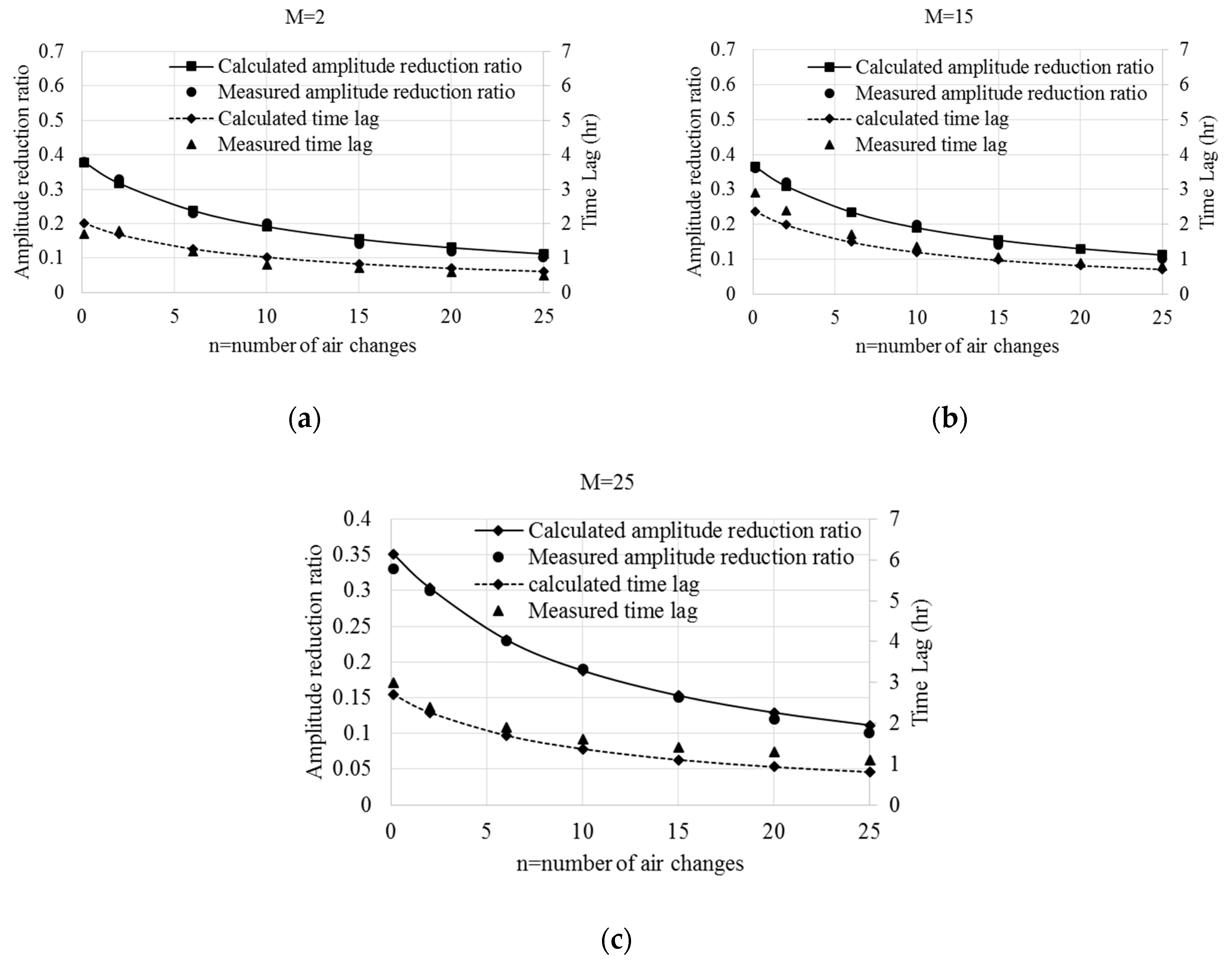
The reported graphs in Figure 5 show the amplitude reduction ratio and the phase shift of a tested wall with different thermal capacities. Looking at Figure 5, it is possible to deduce that the model was accurate for a broad range of air changes, which largely comprehends the values that are currently used in common applications. The model generates accurate results for any value of the internal thermal capacity referred to the unit area of the walls being tested, M, assuming, as previously said, values of 2, 15, and 25 [kJ/m²K].

Regarding the graphs, it is easy to understand the positive effect of the air changes on the amplitude of the temperature oscillations: The amplitude of the temperature oscillations almost halved when the air changes were varied from 0.5 to 10. Besides, for air changes lower than 5, the net reduction of the amplitude of oscillation was affected to a larger extent by the thermal capacity of the room content.

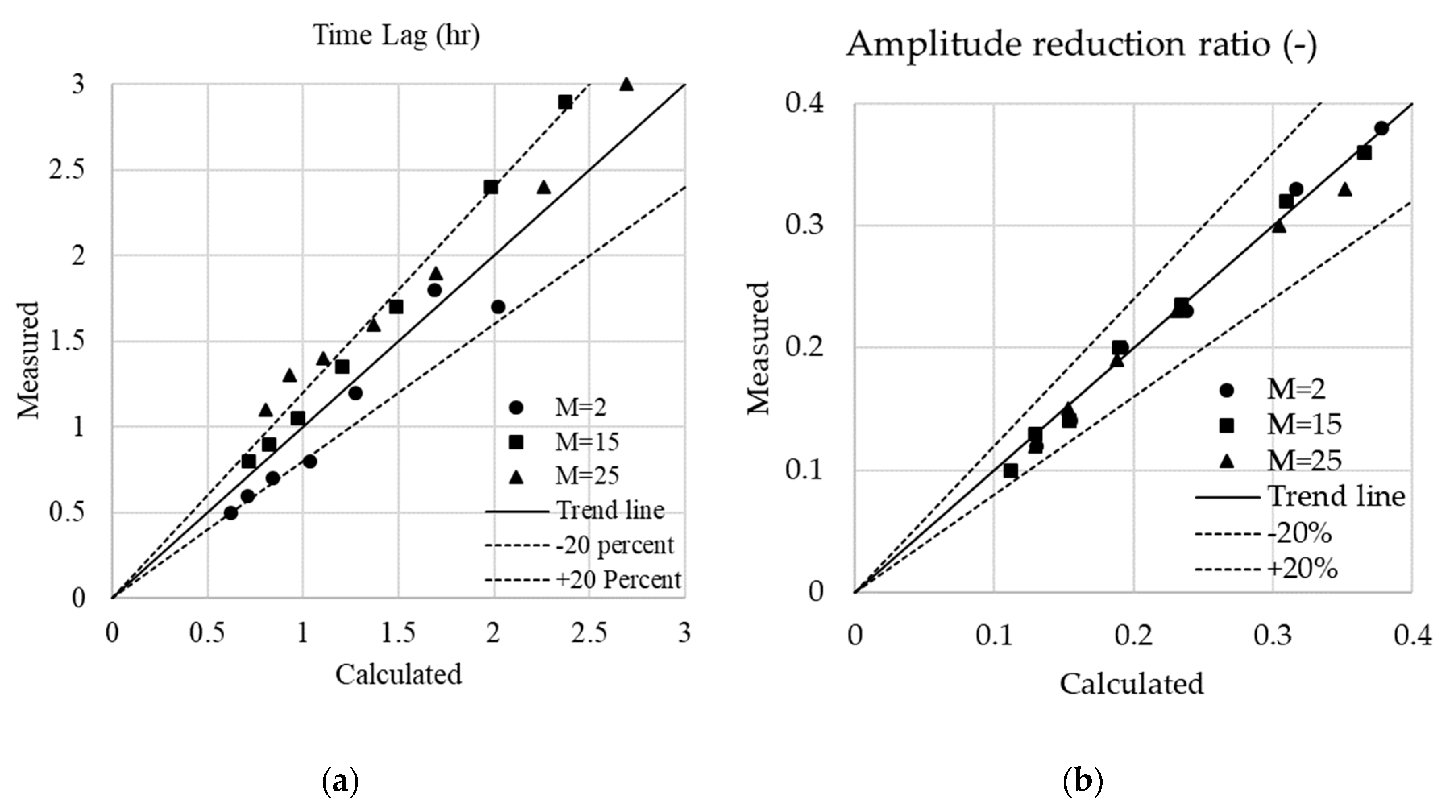
Figure 6 reports the measured value and the corresponding numerical results, in order to highlight the accuracy of the model.

The accuracy of the predictive model was evaluated according to two criteria: The fractions of data predicted to within ±20%, called ϕ, and the mean absolute percent error, MAPE, defined by Equation (13):

$$MAPE=\frac{100}{n}{\displaystyle \sum }_{t=1}^n\left|\frac{A_t-F_t}{A_t}\right|$$

(13)

here A_t is the measured value and F_t is the calculated value.

The calculation of these two quantities shows that for the time lag simulation ϕ = 0.762 and MAPE = 15.6%, whereas for the amplitude reduction simulation ϕ = 1 and MAPE = 5.1%; for the simulated amplitude reduction results, the fraction of data predicted to within ±10% was equal to 0.81.

5.1. Steady-State Simulation of Different Wall Configurations

The second set of experimental results, which was used to validate the numerical models, was taken from the paper by Fiorato and Cruz [40].

During tests in steady-state conditions, the chambers were maintained at a constant temperature and the wall was exposed to a steady differential temperature. The temperatures were kept constant for a proper time until the steady-state condition occurred. In the Simulink model, the indoor chamber air temperature was controlled at 22 °C; the outdoor air was kept at a constant value to obtain a difference of temperatures equal to −45.6, −28.9, −17.8, 1.7, and 26.7 °C.

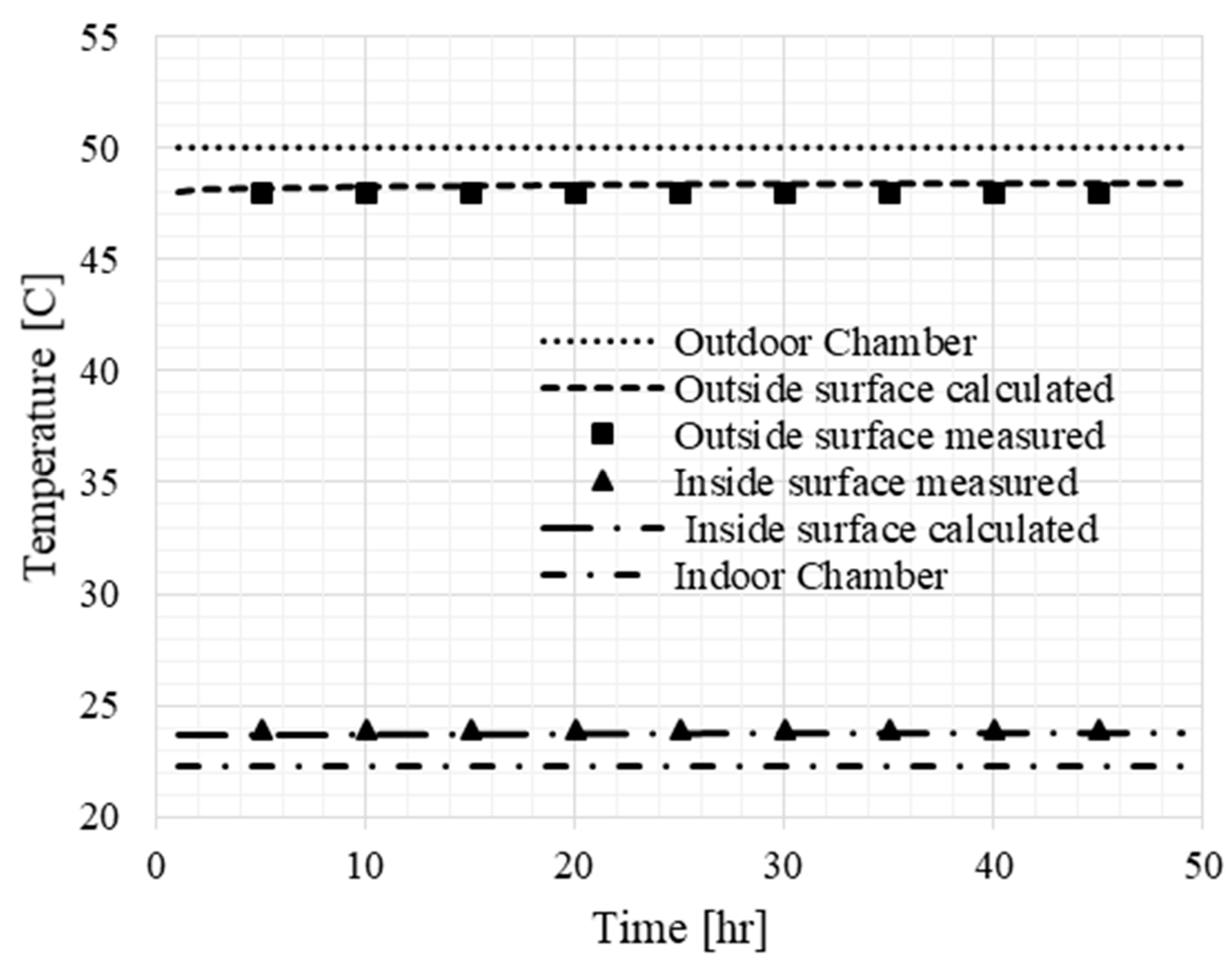
Figure 7 shows the comparison between the experimental values and the calculated ones, for a steady-state temperature difference and the wall configuration number 4 (block brick cavity).

The temperature of the indoor chamber was 22 °C, while the outdoor temperature was 50 °C [40]. The MAPE for this simulation was equal to 0.72%.

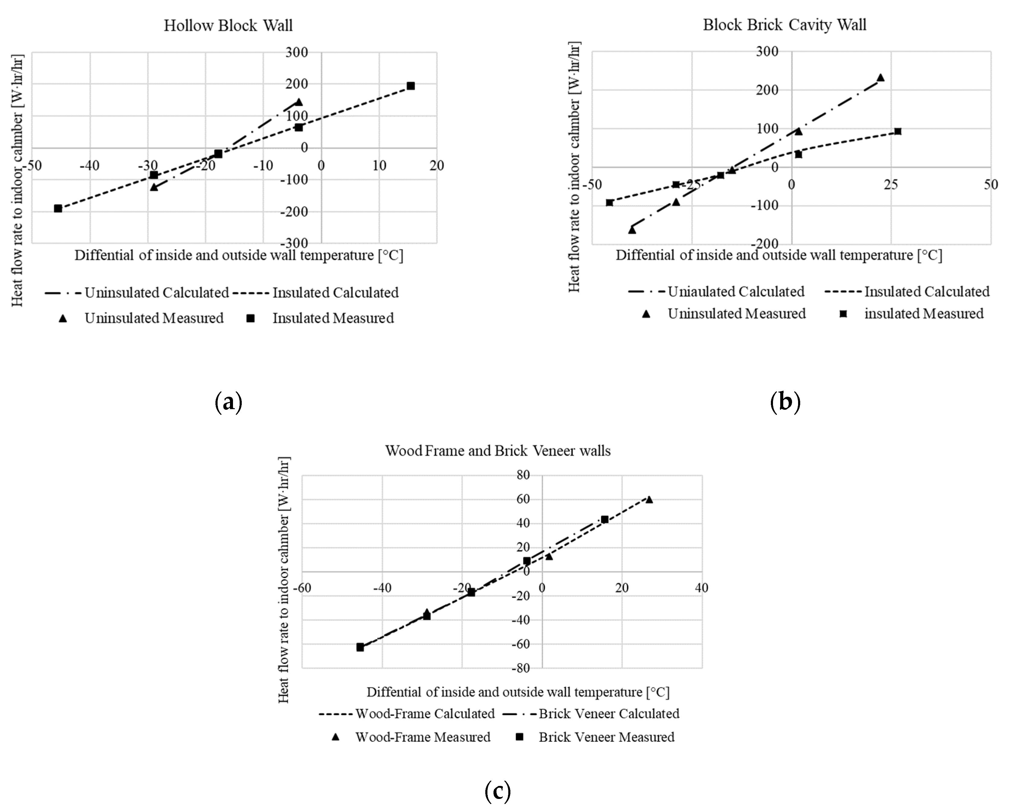
Figure 8 shows a steady-state condition of heat flow rate to the indoor chamber for (a) hollow block, (b) block brick, and (c) wood frame and brick veneer. As expected, the simulations showed that insulation leads to a significant reduction of energy consumption. Moreover, the figures present good correspondence between the numerical and experimental results.

For these three steady-state simulations, described in Figure 8, the MAPE was equal to 17.04%, while ϕ was equal to 0.786.

Table 3. Simulink and test value of resistant and transmittance with six different types of walls.

Specimen	Measured Data [40]		Calculated Data		UEXP/USIM
	R (K m2/W)	U (W/m2 K)	R (K m2/W)	U (W/m2 K)
Hollow block uninsulated	0.49	2.04	0.4	2.501	0.82
Hollow block insulated	0.79	1.27	0.84	1.19	1.06
Block brick cavity uninsulated	0.63	1.59	0.599	1.667	0.95
Block brick cavity insulated	1.5	0.67	1.499	0.667	1.00
Wood frame	2.61	0.38	2.285	0.438	0.87
Wood frame brick veneer	2.78	0.36	2.448	0.408	0.88

illustrates the calculated and measured [40] value of resistance and transmittance for six different types of wall. The last column of the table reports a measured and calculated transmittance values ratio. The calculated data agreed with techniques recognized by the American Society of Heating and Air-Conditioning [41].

According to the table, the transmittance of the insulated hollow block wall was 50% less than that of the uninsulated hollow block. The data obtained showed a close matching between insulated and uninsulated block-brick. In addition, Simulink values indicated the transmittance of the veneer wall was around 90% of the wood frame.

5.2. Dynamic Model

The assessment of the dynamic model was focused on the daily temperature variations, because this is the timescale at which the transient behavior of buildings determines the thermal comfort and the energy consumption. For this reason, the model was used to simulate the condition of a two-day experiment, whose results were available in literature.

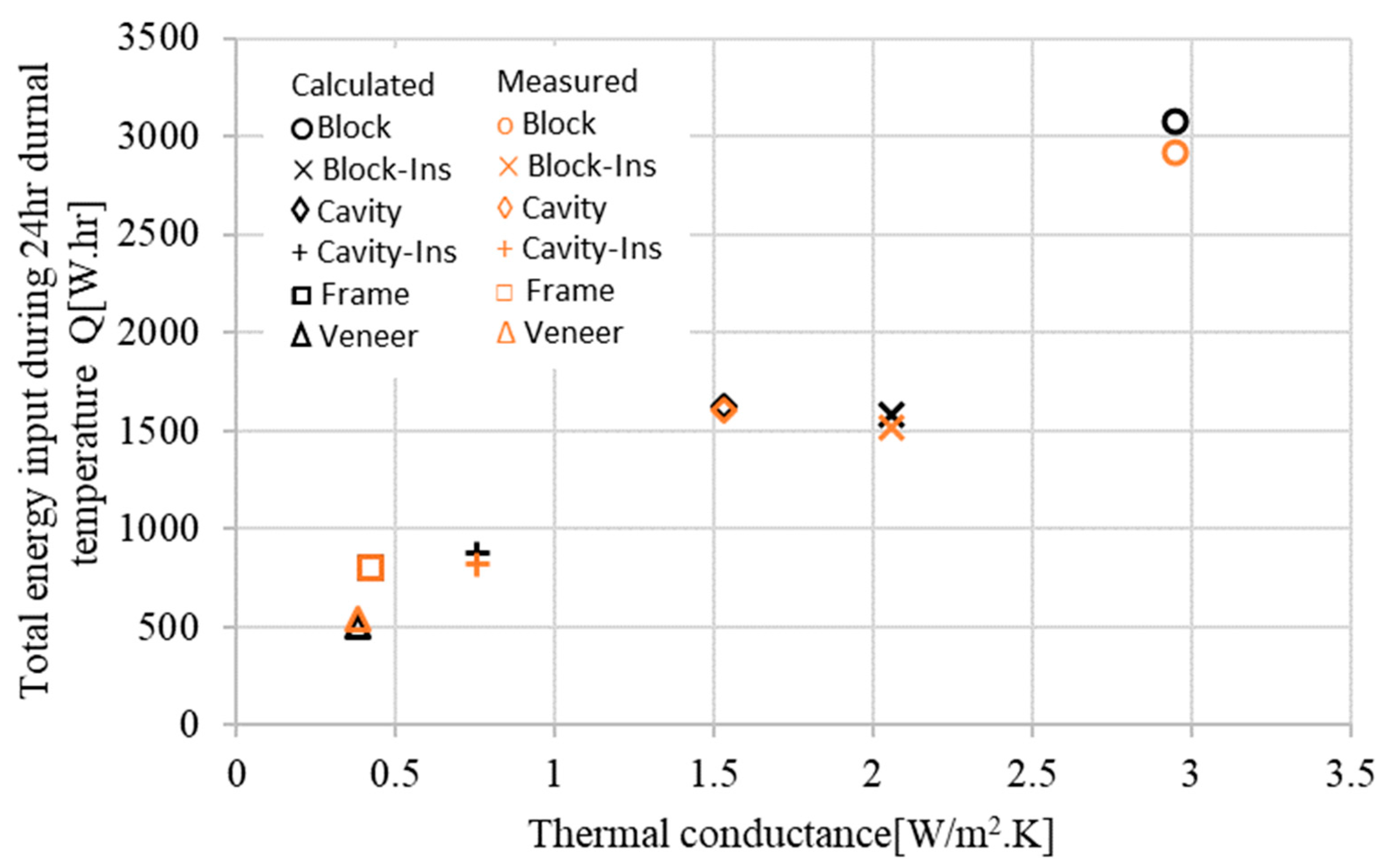
Figure 9 shows the total energy response for 24 h as a function of the measured average thermal conductance of the walls. The results show that the amplitude of periodic heat flux was influenced by the thermal conductance of the wall. In addition, the maximum and minimum response were related to block and veneer, respectively.

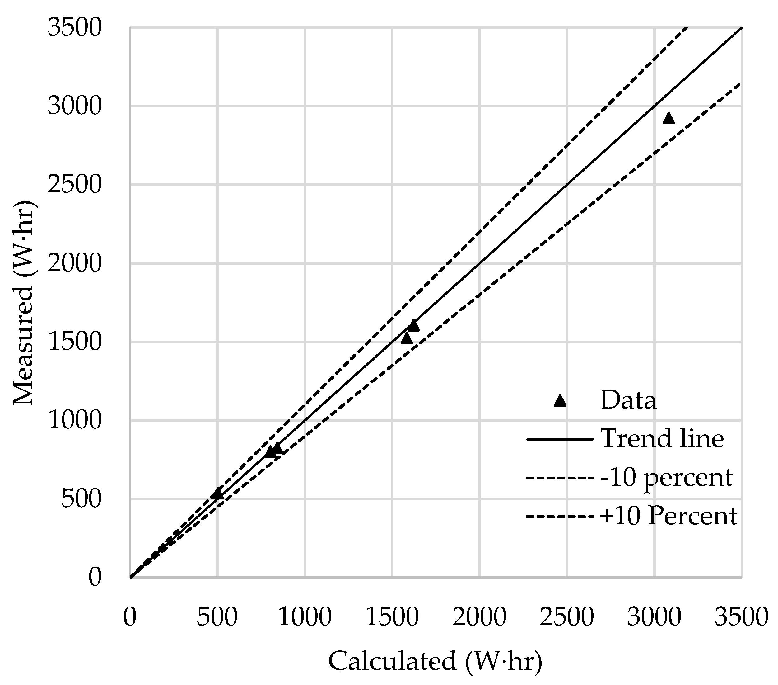
The model again showed very good agreement with experimental data: As shown in Figure 10, for this kind of dynamic simulation the fraction of data predicted within 10% was equal to 1, while MAPE = 3.1%.

Finally, a simulation was conducted in order to evaluate the heat flow rate vs. time during a day. Using, as the input, the same diurnal sol-air temperature cycle of [40], the variation of the heat flow rate during 24 h was calculated in terms of heat flow rate to indoor chamber with t₁ − t₂ ≠ 0, called Q_t, and heat flow rate to indoor chamber with t₁ − t₂ = 0, called Q₀, where t₁ and t₂ are, respectively, the average temperatures of inside and outside wall surfaces.

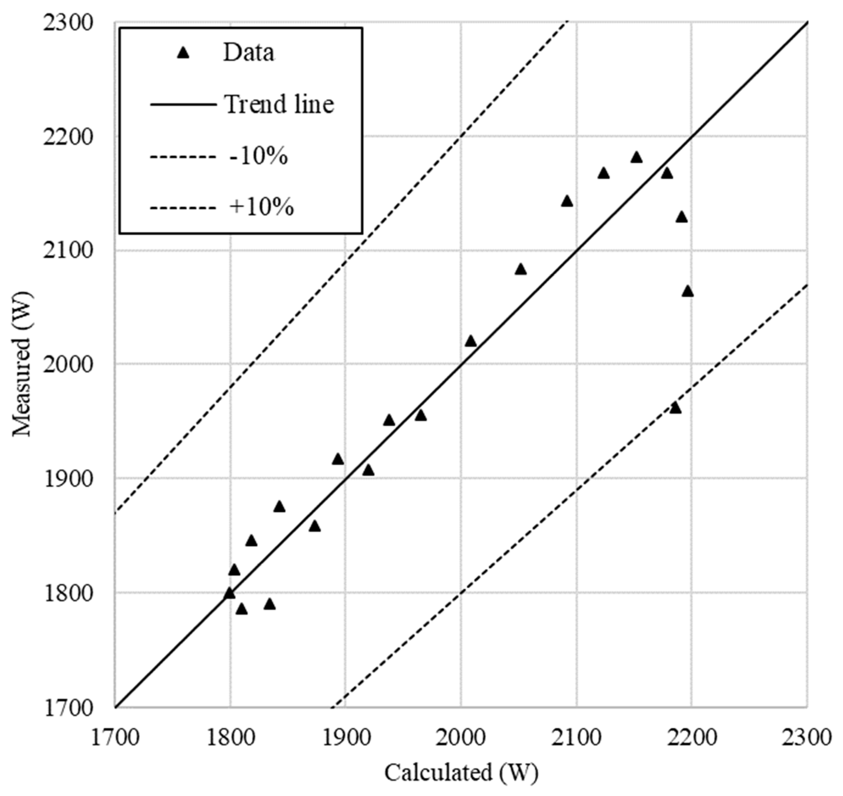
At a general glance, Figure 11 shows that there was a very good agreement between measurements and calculations: For this dynamic simulation, the MAPE was equal to 2.04% and the fraction of data, predicted to within ±10%, was equal to 0.95 (Figure 12).

6. Application of the Model

The preliminary activity led to the validation of the model’s capability of performing a numerical simulation of the dynamic behavior of a typical wall, in circadian transient conditions. For this reason, the model was used to investigate an interesting case study.

A typical single-zone building was selected in order to investigate the performance and capabilities of the developed model. The building had the features of a typical residential building located in the surroundings of Genoa, Italy. The apartment was in the middle of a three-floor building.

In addition, the “single-zone” had two walls in common with other neighbors and two different ones facing outwards that were exposed to the external air and to solar radiation.

Two cases will be studied in the following: The first one takes into consideration a period of one week, made up of seven different daily profiles of temperature with circadian oscillations; while the second one analyzes the thermal behavior of a leisure house (i.e., used, for example, on weekends only), for different powers of the heaters and for different outdoor temperatures, in order to analyze and speculate about the possibility of saving energy by means of remote control of the plant.

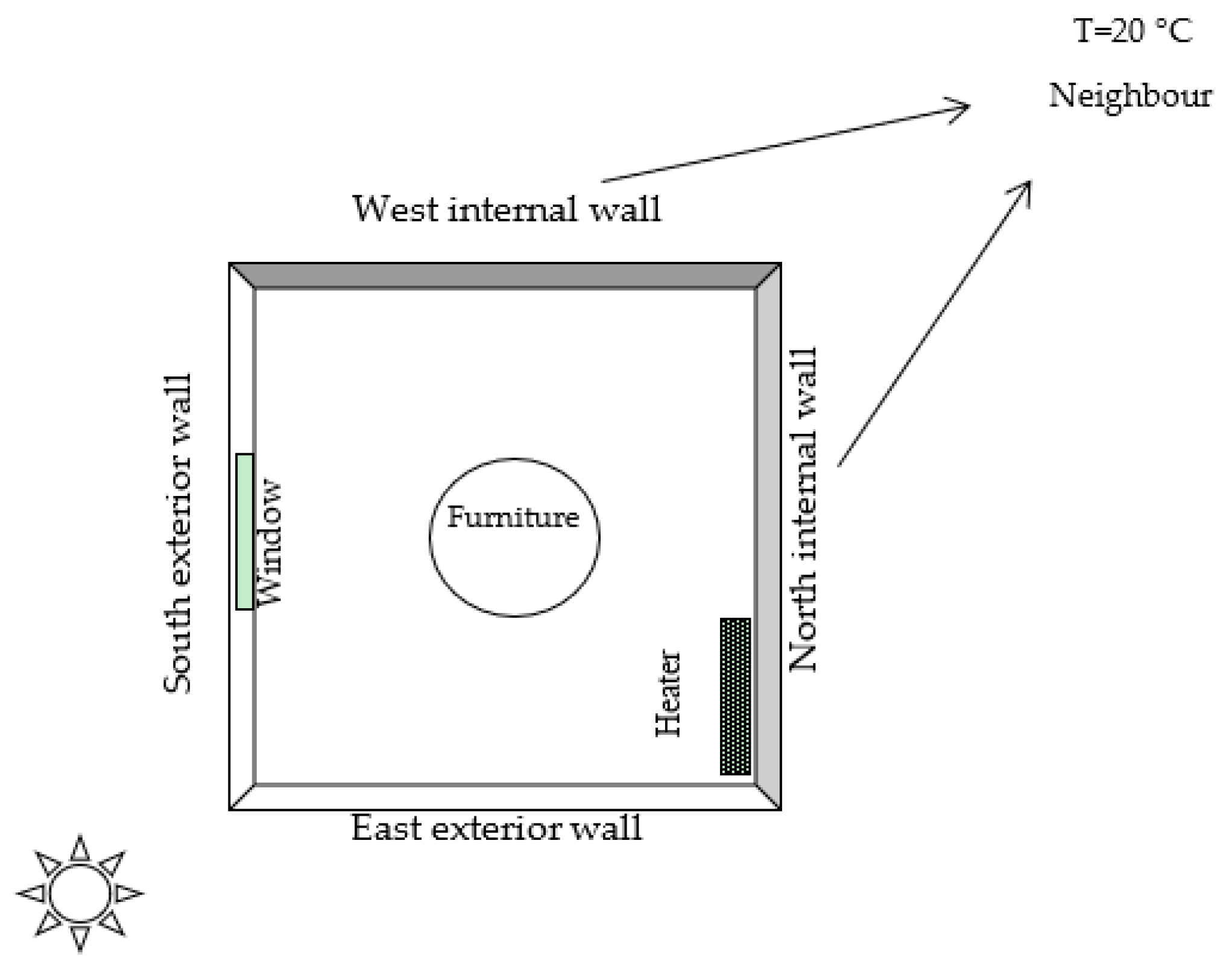
The sketch of the single zone is shown in Figure 13 and the general conditions, dimensions, and boundary conditions are shown in

Table 4. General conditions.

Properties
Building location	Between two floors
Dimensions (m)	4 × 4 × 2.7
Window dimensions (m)	1 × 1 × 0.02
Exterior wall	5 layers
Internal wall	3 layers
Boundary conditions	Internal wall outside temperature 20 °C

.

Thermal properties of the exterior, internal walls, roof, and floor are presented in

Table 5. Thermal properties of exterior wall layers (MCV01) [42].

Materials	Thickness (m)	Density (kg/m3)	Thermal Conductivity (W/m·K)
Exterior plaster	0.02	1800	0.9
Hollow brick	0.25	800	0.281
Air gap	0.03	1.246	0.025
Hollow brick	0.1	800	0.385
Interior plaster	0.02	1400	0.7

,

Table 6. Thermal properties of interior wall layers.

Materials	Thickness (m)	Density (kg/m3)	Thermal Conductivity (W/m·K)
Exterior plaster	0.02	1000	0.9
Brick	0.10	2000	0.281
Interior plaster	0.02	1000	0.9

,

Table 7. Thermal properties of roof layers, SOL02 [42].

Materials	Thickness (m)	Density (kg/m3)	Thermal Conductivity (W/m·K)
Interior	0.015	1700	1.47
Cement	0.02	2000	1.4
Lightweight concrete	0.12	1400	0.58
Cement	0.02	2000	1.4
Brick-block concrete	0.24	900	0.69
Interior plaster	0.02	1800	0.9

and

Table 8. Thermal properties of floor layers, SOL02 [42].

Materials	Thickness (m)	Density (kg/m3)	Thermal Conductivity (W/m·K)
Interior plaster	0.02	1800	0.9
Brick-block concrete	0.24	900	0.69
Cement	0.02	2000	1.4
Lightweight concrete	0.12	1400	0.58
Cement	0.02	2000	1.4
Interior	0.015	1700	1.47

(where a code is indicated, it refers to the standard UNI/TR 11552:2014 [42]).

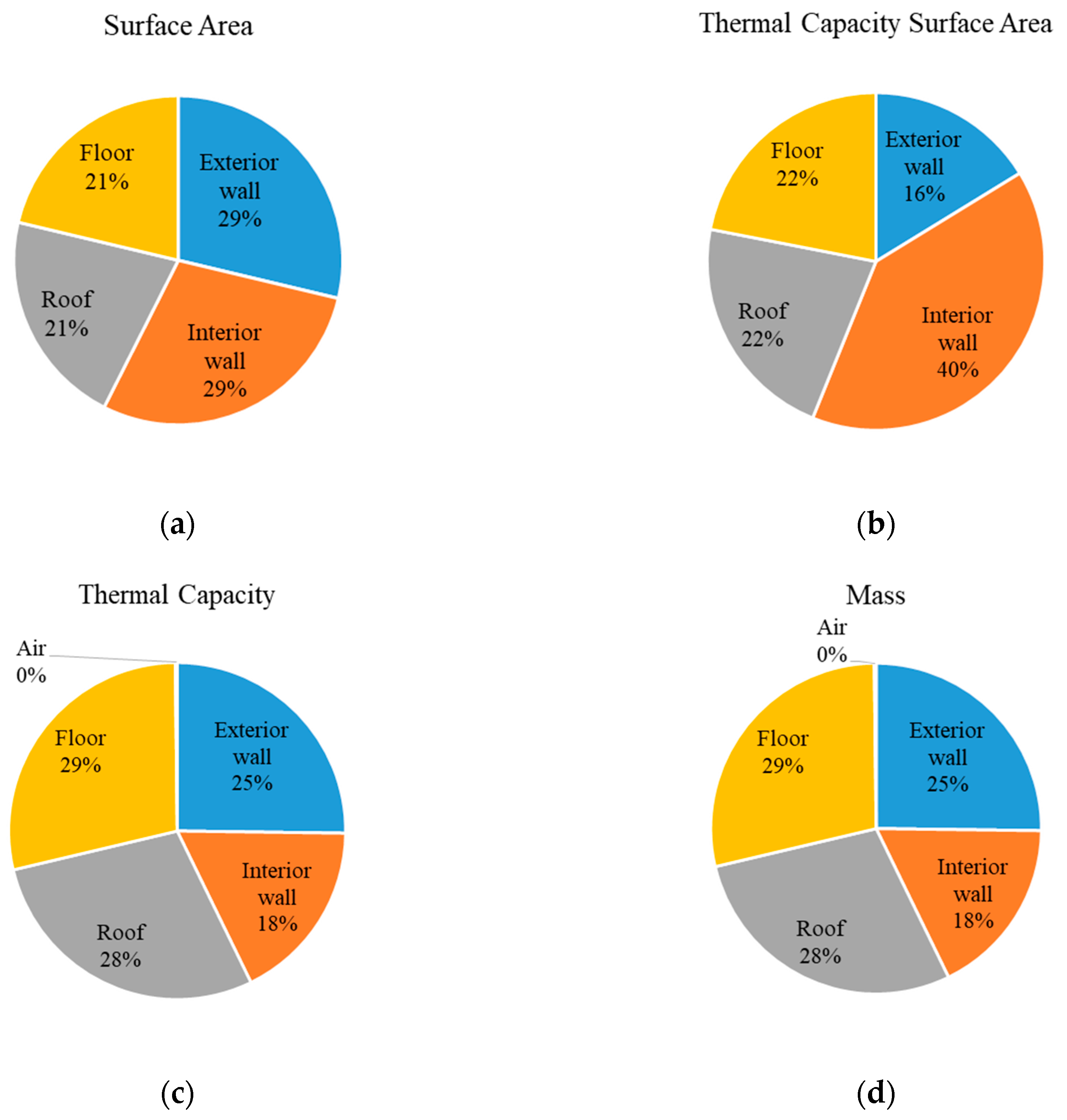
Four pie charts are displayed, in Figure 14, in order to summarize the common configuration of the considered single-zone building. They describe the thermal properties of the various parts of the building.

It is possible to deduce that each part had a different weight in the various physical processes. For instance, the maximum weight of thermal capacity was accounted for by the roof and floor, while most of the surface area was allocated to the exterior wall.

In order to investigate the application of the developed model, another case study was generated. In this study, an insulation layer with embedded PCM was used for all the surrounding walls. PCMs are well-known as a new generation of insulating materials, applied in order to absorb the daily energy and then release it at night. In previous studies, authors deeply studied, both experimentally and numerically, the use of PCMs [11,12,43,44].

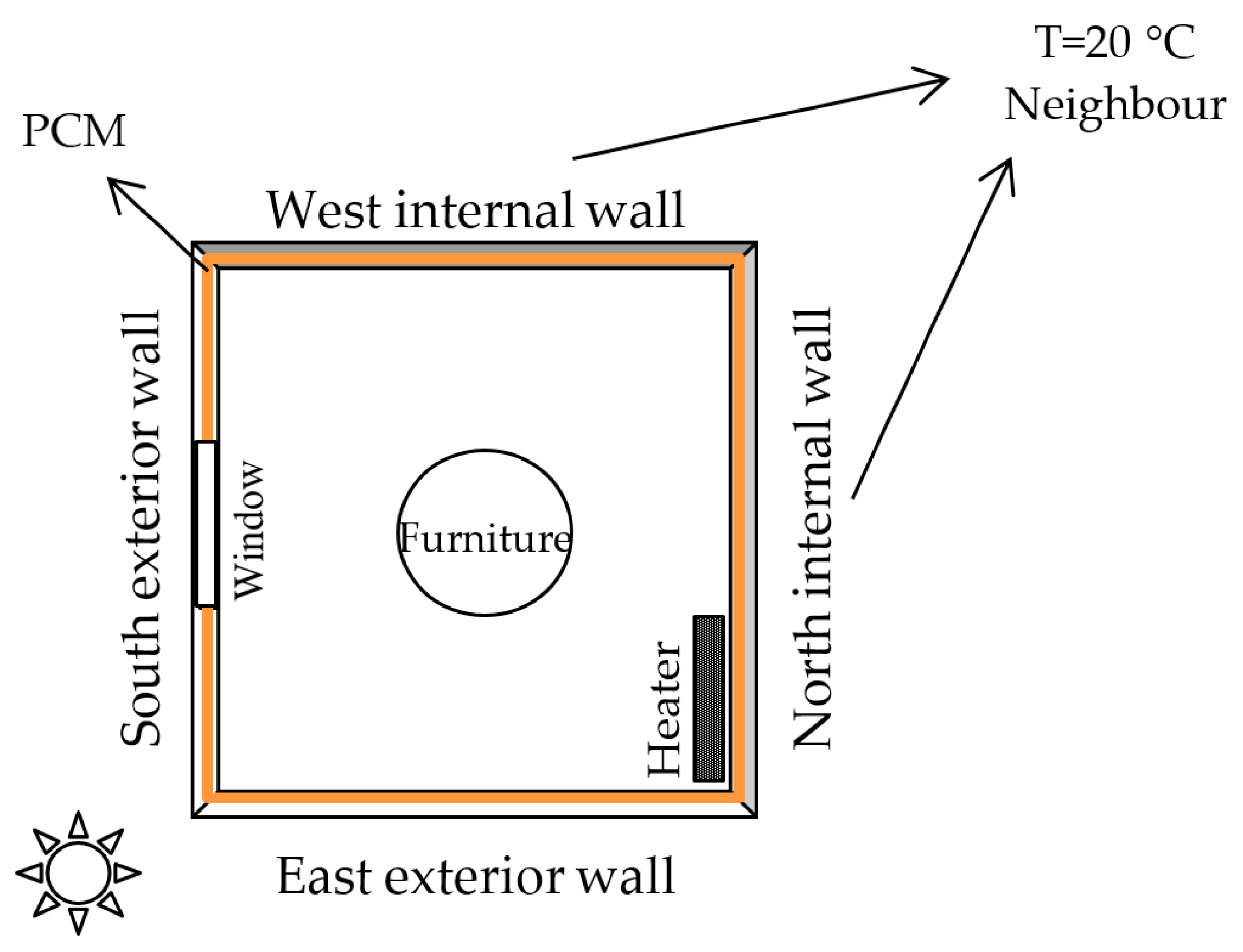
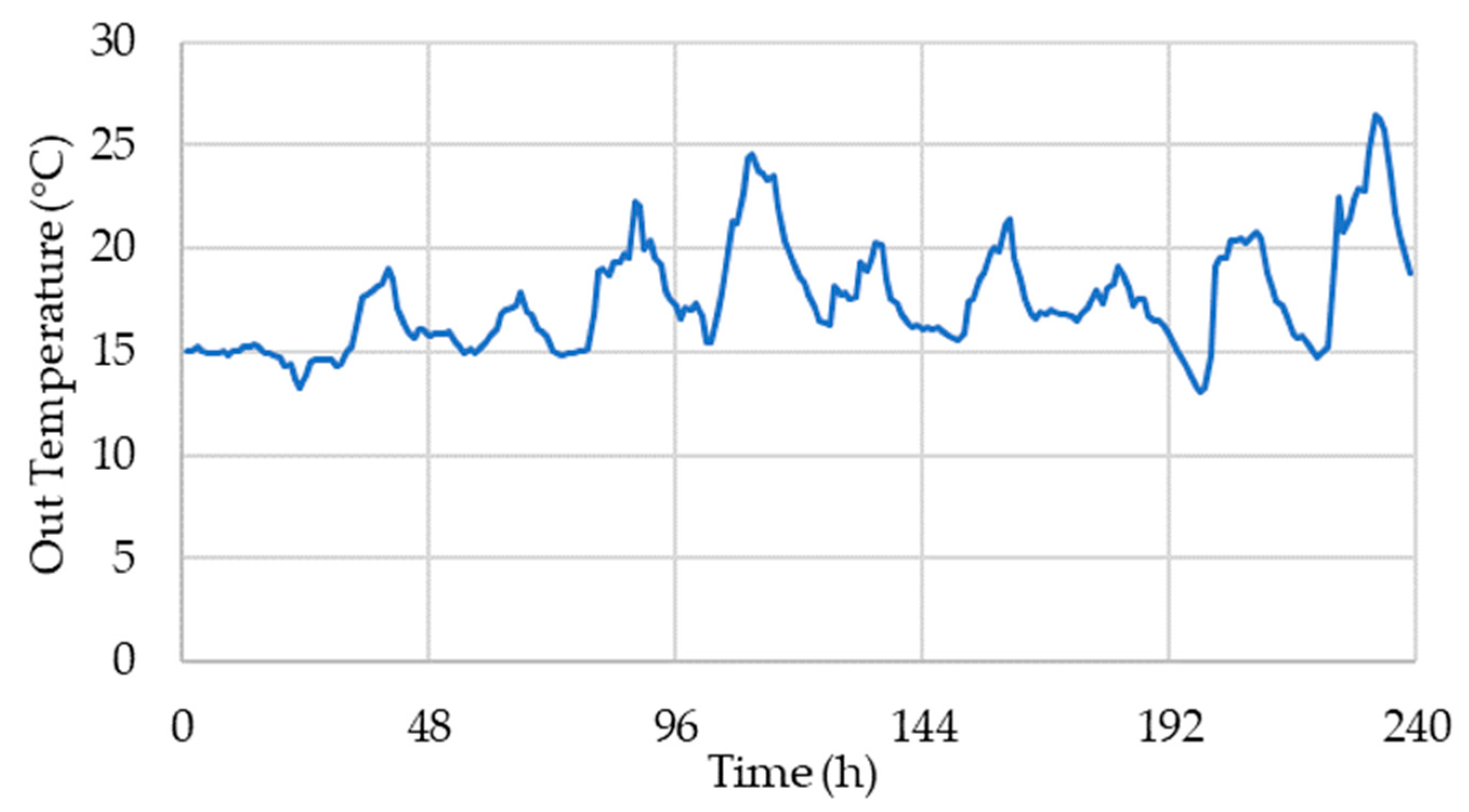
Figure 15 shows the schematic of the building’s embedded PCM; in this model the PCM was placed close to the inside layer of the walls. The outside temperature and the characteristics of the used PCM are shown in Figure 16 and

Table 9. PCM specifications.

Material	Specific Heat Capacity (J/kg·K)	Density (kg/m3)	Thermal Conductivity (W/m·K)
Energain® PCM	variable	855	0.18, 0.23

.

In this model was also taken into account the hysteretic behavior of PCMs, already deeply described in references [11,12] and [43,44], in order to achieve accurate results in a proper time.

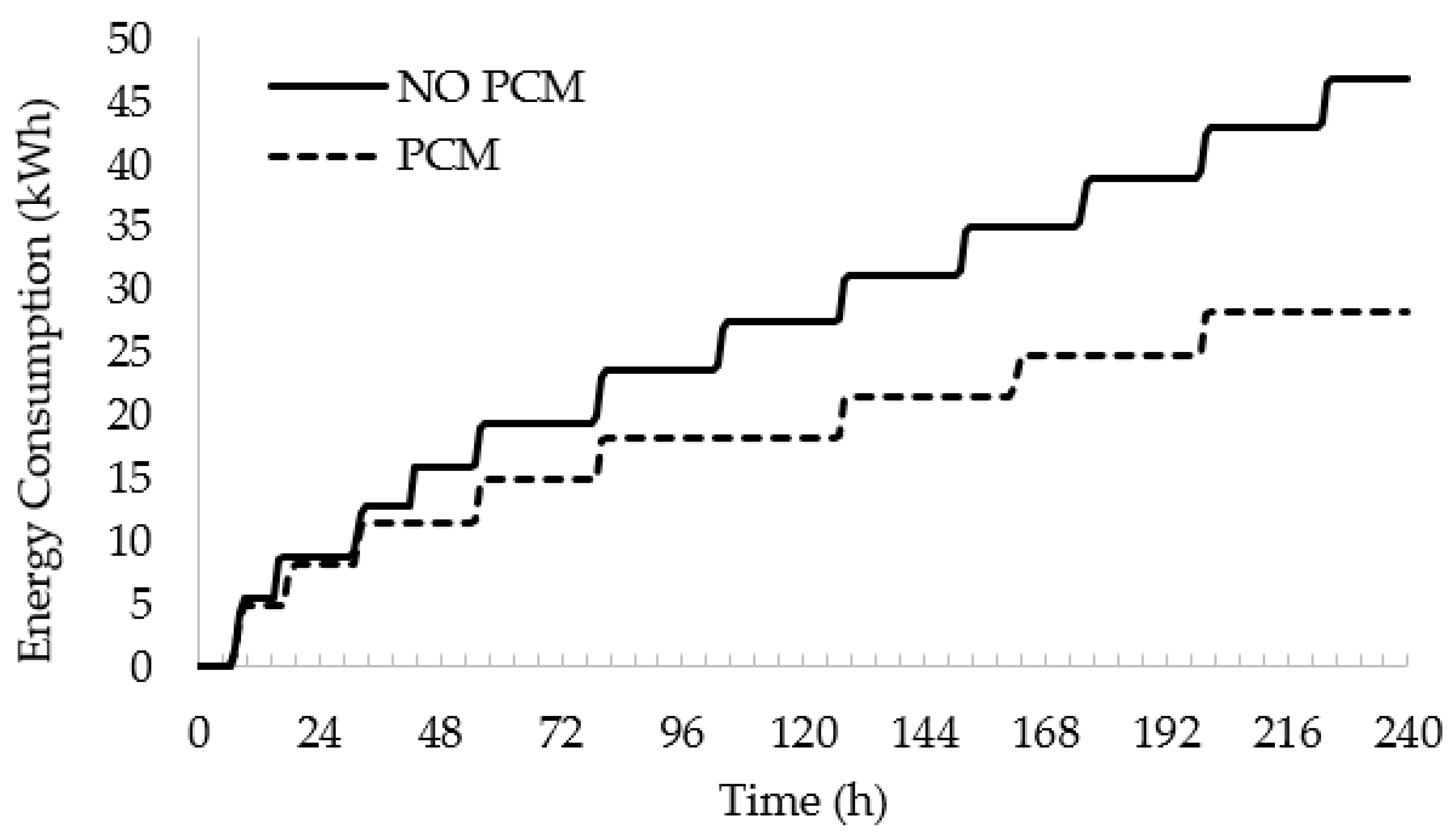
In this way, the energy consumption of the single-zone house was obtained. Figure 17 illustrates the amount of energy consumption for 10 days in the building in two different cases:

(1)

Without PCM insulation;

(2)

With a PCM insulation layer.

The obtained results showed that during the first two days, when the outside temperature was lower than the melting temperature, the amount of energy saving was not significant. On the other hand, the increasing rate of energy consumption in the building, when using the PCM, was moderately lower than the one of the building without PCM.

7. Results and Discussion

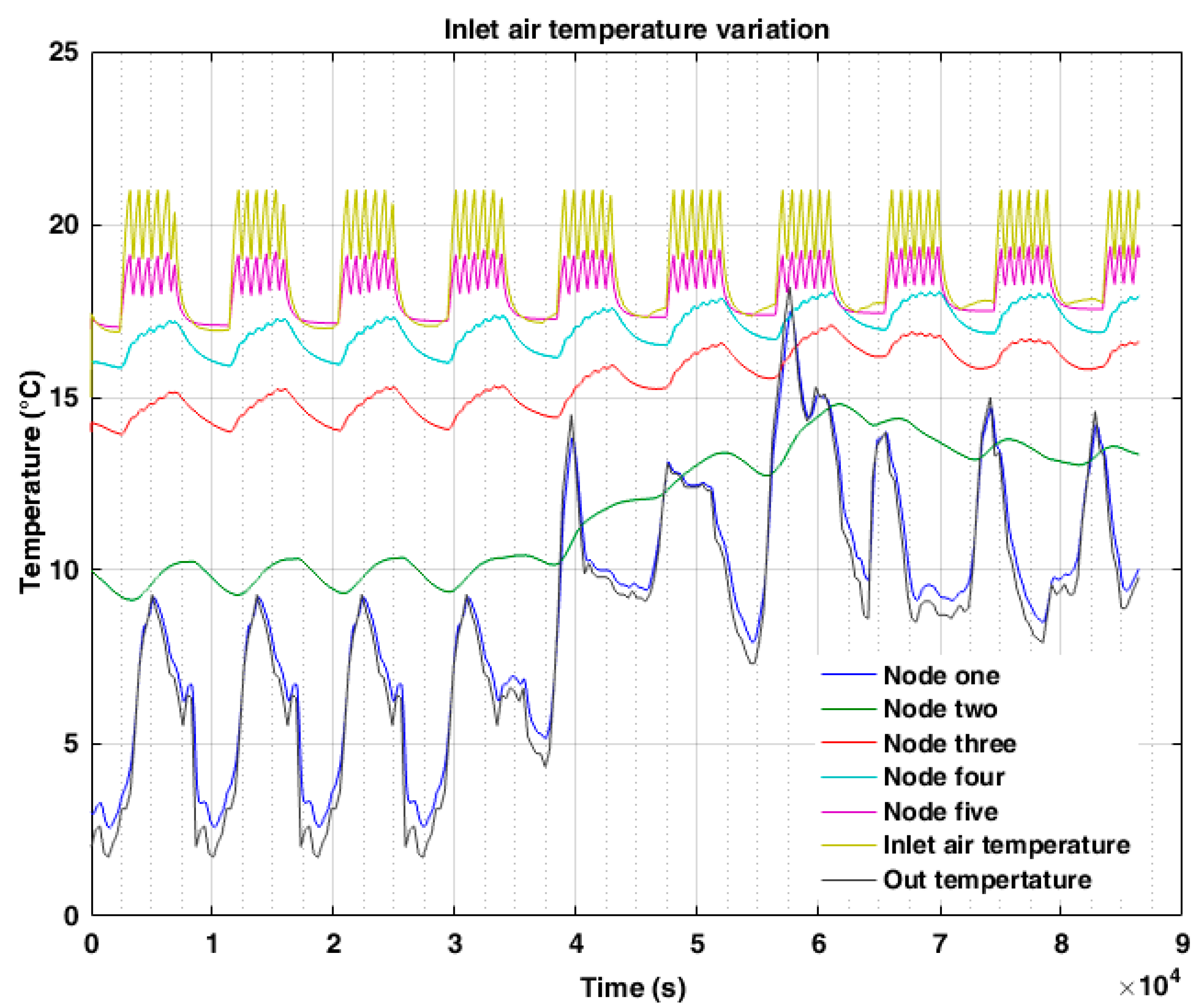
The model was used to investigate some cases, whose dynamic behavior in transient condition was considered to be of relevant interest. The first case took into consideration a period of one week, made up of seven different daily profiles of temperature with circadian oscillations. In practice, the simulation was extended to a 10-day period, in which the first day was repeated three times at the beginning, to get to a stabilized quasi-periodic condition and to eliminate a possible bias, which might be have been induced by an initial unphysical distribution of the temperature of each layer. For this reason, the significant results were gathered for one week long, from the third day onwards. A thermostat controlled the heater by means of a simple on–off logic, with a ±1.0 °C activation band and a set point at 20 °C. Similar to a relay, the heater’s switch-on point was at 19 °C and the switch-off point was at 21 °C, during the day. Analogously, at night, the set point was at 17 °C.

Figure 18 illustrates the temperature variation of each layer of the external walls for ten days, together with the external and internal temperatures. The results show that the Simulink model controlled the internal temperature of the considered building between 19 to 21 °C, whereas the external temperature fluctuated between 2 and 17 °C. The temperature of the inner layers gradually increased and then decreased, following the fluctuations of the external temperature in a smooth way, between the fourth and seventh days. The thermal variation of the external layer was close to the external temperature, and the amplitude of fluctuation within this layer was the highest between the layers. In fact, each layer decreased the rate of fluctuation, from the outer to the inner layer. In the presence of the night time set point, fixed at 17 °C, the building exploited the high thermal capacity and the heater remained switched off, all night long, until the daytime set point was restored. Besides, it can be seen precisely that the fluctuations of the nodes near the outer layer were greater than the internal nodes, and the variation of node two slightly increased when the outside temperature increased.

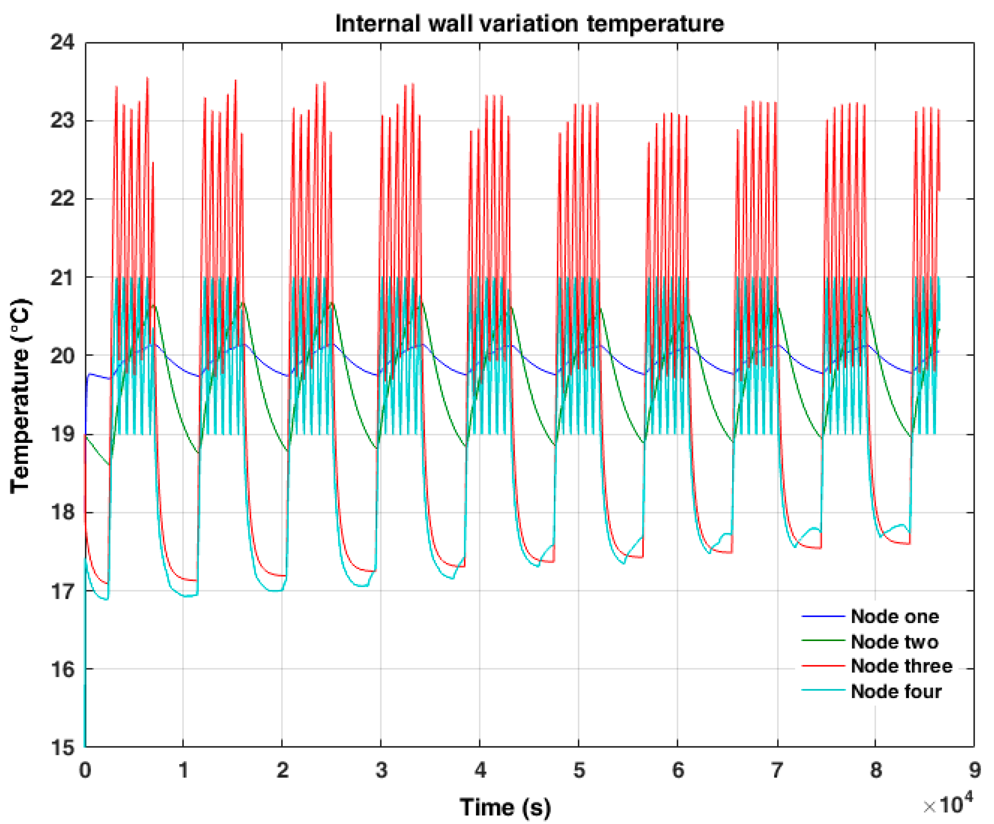
Figure 19 shows the temperature variation of an internal wall. The profile of node three, red in Figure 19, represents the mean radiant temperature, including the heater surface. On the other hand, while the outdoor temperature was increasing, the minimum temperature of node three and four gradually increased.

The second case describes the thermal behavior of a country house, located in the countryside or in the mountains, used for leisure or at weekends, in a non-continuous way, for pleasure.

It was assumed that the apartment was empty at the beginning of the simulation, as well as the surrounding ones.

The initial internal temperature was fixed at 6 °C; the internal initial temperature corresponds to the set-point common no-icing controls, which maintain the internal temperature of the house always higher than 5 °C, in order to prevent the formation of ice in the pipes and their consequent rupture. The simulations were accomplished in case of three different heater powers and a set of outdoor temperatures: 0, 5, 10, 15, and 20 °C.

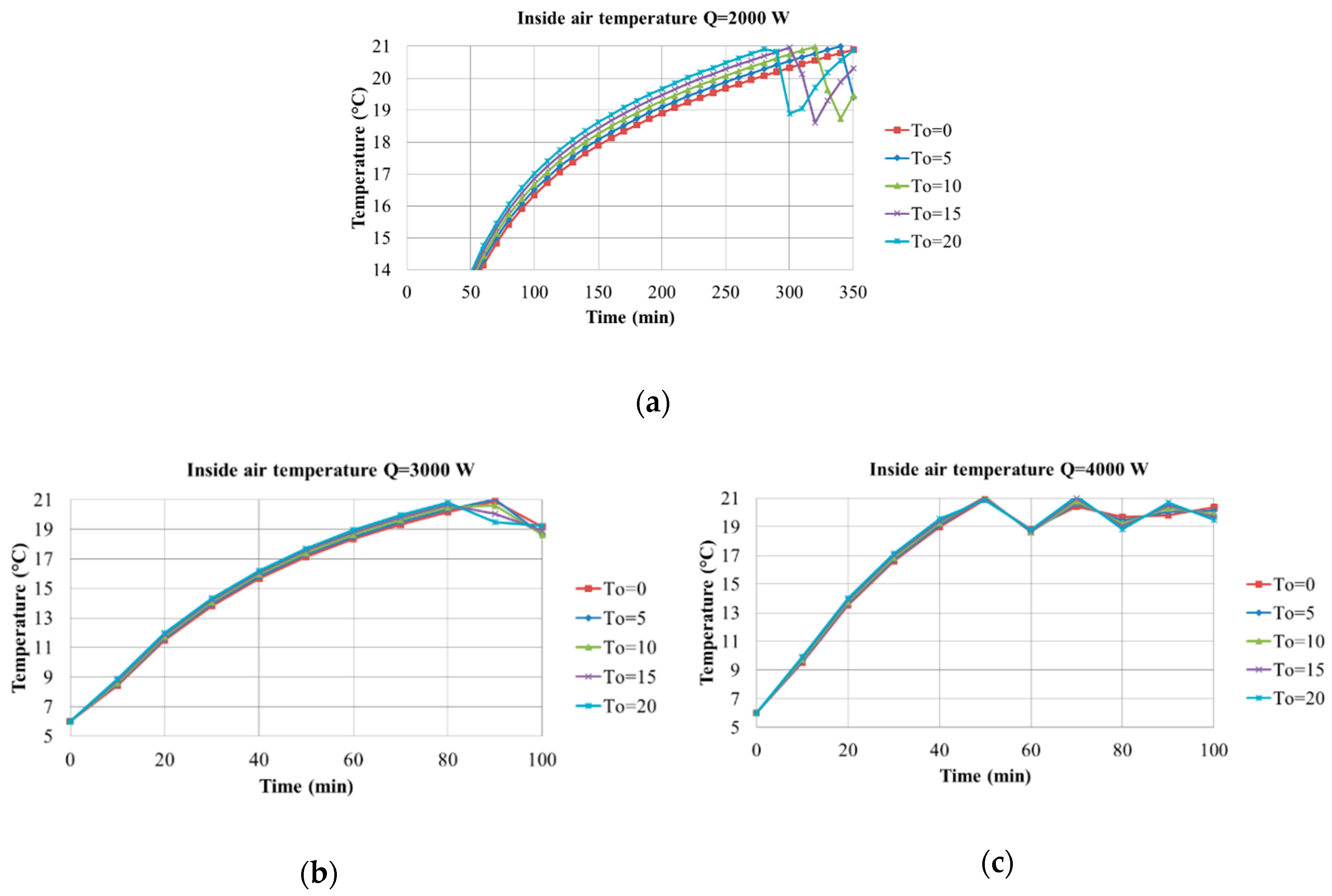
The graph in Figure 20 shows the starting transient condition for the internal air temperature of the building, which was calculated for a set of different cases. The cases, which were considered, differed one from another for the maximum thermal power of the heater and for the temperature of the external environment. At first glance, it was easy to appreciate that the time, which was needed to achieve thermal comfort, sharply decreased as the power and the outdoor temperature increased.

Figure 20a shows that in case of outdoor temperature equal to 0 °C, the internal temperature reached 21 °C, in about 350 min. The time needed to get to thermal comfort decreased to 280 min if the outdoor temperature increased from 0 to 20 °C. In graph (b), the power was 3000 W and the time significantly decreased to 90 min, for an external temperature equal to 0 °C. Moreover, graph (c) shows that the delay dropped to 50 min for a power equal to 4000W.

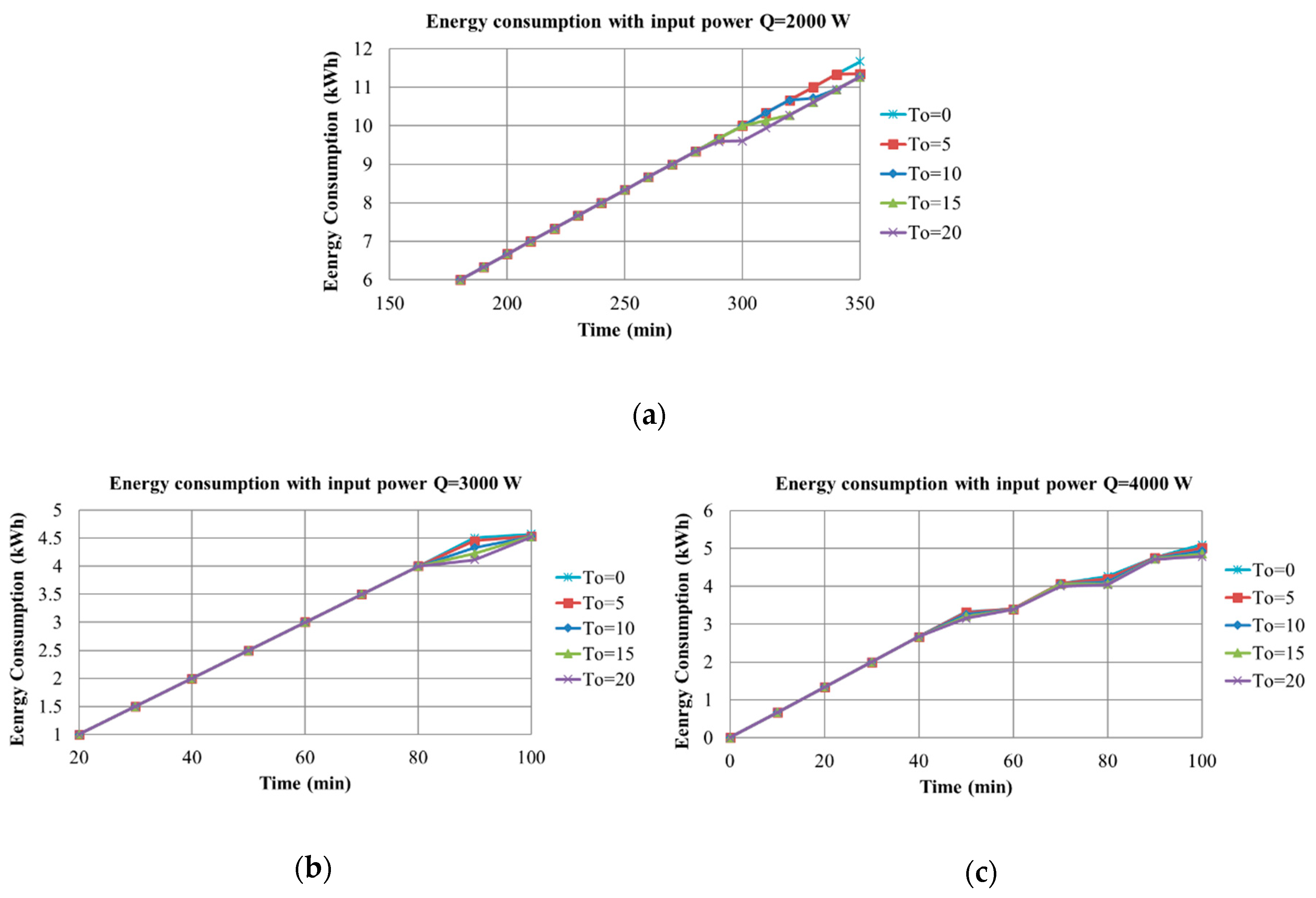
Figure 21 shows the energy consumption in the building in order to achieve the temperature of 21 °C, with variable input power and external temperature. If we think about a domestic plant, which is remotely controlled (activated), in advance, to guarantee the thermal comfort conditions at a predefined time, the lower the power of the heater is, the longer the plant must be turned on in advance. For this reason, the higher energy consumption was obtained with the heater power of 2000 W, about 11.3 kWh, because the heating period, which leads to the comfort condition, was longer. The power consumption for the other input powers considered were 4.5 and 3.2 kWh, respectively. It is worth noting that, if one thinks of switching on the plant in advance to achieve thermal comfort when one arrives, the larger the heater power is, the less they consume. The fluctuation on the graphs after reaching the comfort temperature were due to the on/off control.

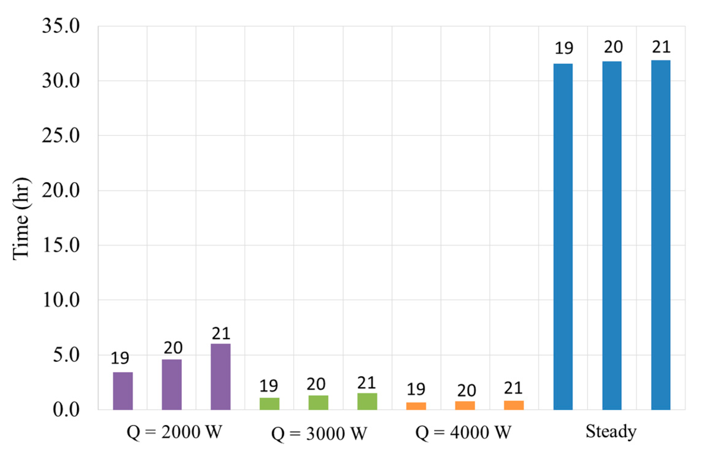
Figure 22 shows the amount of time that was needed to reach the final comfort state, for many different conditions. The different colors of the bars represent the different powers of the heating system. On the other hand, the numbers on the bar are the internal temperature set-points that were investigated (19, 20, and 21 °C). The big blue bars on the right side represent the time that would be needed if the size of the heating system was exactly equal to the required amount for steady-state condition. In the case whereby the heater power was exactly equal to the one required at steady-state, the duration of the transient would be unacceptably long, and this would make it impossible to appreciate the differences between other bars, if they are plotted together. For this reason, to make it clearer, the results for 2.0, 3.0, and 4.0 kW were separately reported, in

Table 10. Oversizing of the heaters power.

		Suggested Comfort Temperature			Average
		19 °C	20 °C	21 °C
Power	2000	164%	153%	144%	150%
	3000	247%	230%	216%	230%
	4000	329%	307%	288%	310%

.

Today, a wide range of cheap and non-invasive devices, which enable remote control of heating systems, are available on the market. Even the cheapest of these devices can switch on the heating via mobile phone, tablet, or by means of a web interface, and they can also be used in old buildings, which would be difficult and expensive to turn into smart buildings. Bearing in mind the transient conditions, corresponding to what happens when one goes into a cold and unused house, it is possible to imagine that such buildings are placed far from the main city in the countryside or the mountains, and it is possible to switch on the heating before traveling there. In this case, a delay of some hours could be a proper period, for people travelling, to get a thermally-comfortable house. Within this new context, transient analyses are useful tools to evaluate, from a different point of view, the proper power size of the heaters and the percentage of oversizing of heater power in comparison with the one calculated for the steady-state.

Table 10 reports a set of scenarios that were evaluated using the model. In all of these cases, the power of the heaters strongly exceeded the heat flow rate at steady-state. In Table 10, percent oversizing of heaters power is represented, considering different powers of the heating system and different comfort temperatures. The last column of the table shows the average oversizing of the power of the heaters, calculated as the ratio between the effective power and the one needed at steady-state condition (design point).

A clear difference can be seen between the power of 2 kW and small differences between 3 and 4 kW. Using a heater power of 2 kW, the time that it took to achieve the comfort conditions was about five hours (see Figure 23); for this reason, it would be interesting to have smart, remote, or mobile control of the building.

Looking at the thermal power supply of 3 and 4 kW, the duration of the transient was about 1 h in both cases, and the increase of the power of the heaters, from 2.3 to 3.1 times the minimum necessary, did not make a significant decrease in the delay that was needed to get comfortable conditions. If one considers the time of peoples’ adaption in a new environment and can accept short delays, it is possible to conclude that both cases lead to comfortable conditions in a short time, of the order of a quarter of an hour, even if users switch on the heating, with no advance, only when they go into the house.

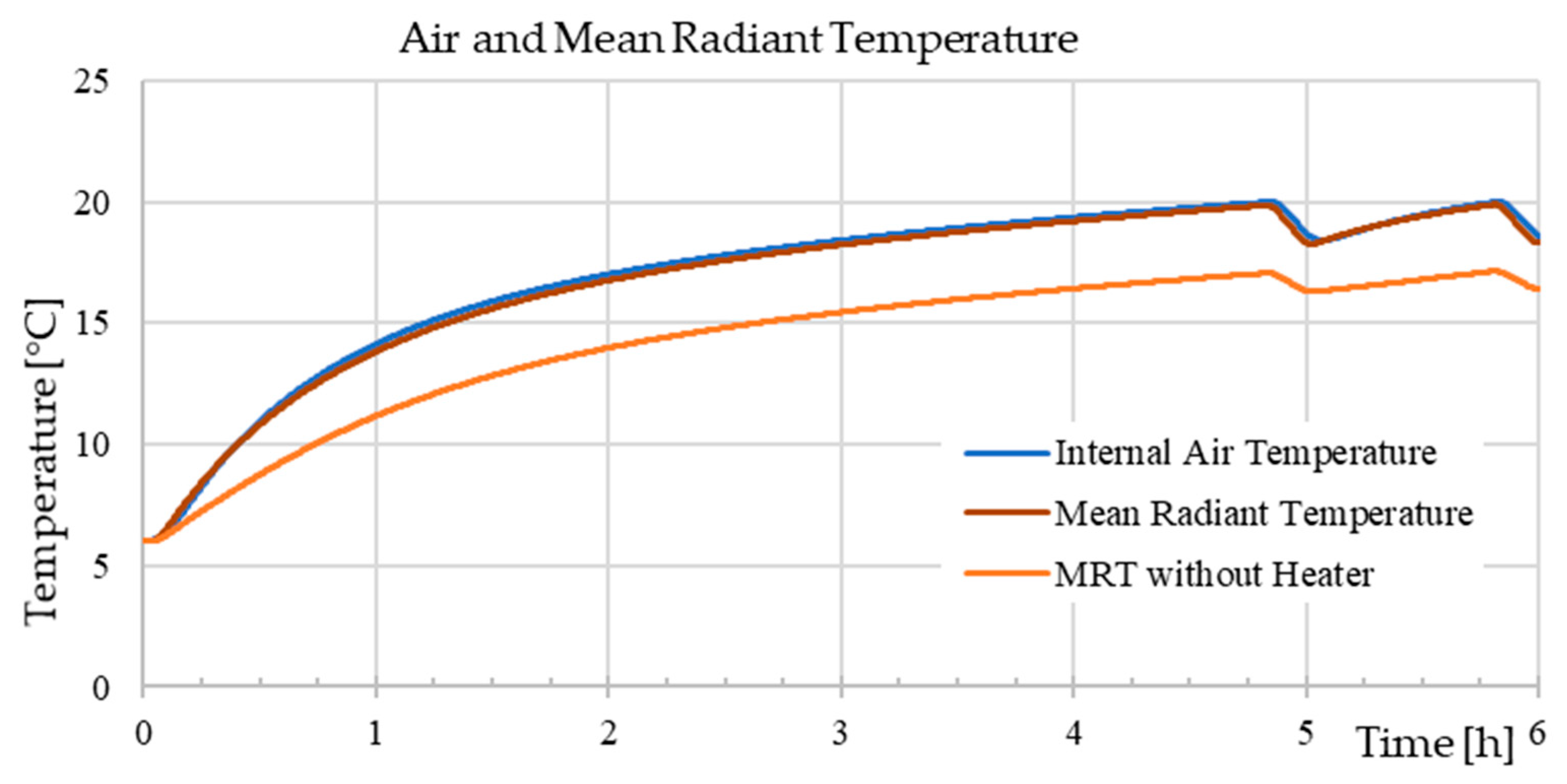
Figure 23 shows the profile of temperature, in time, after switching on the heater with a “cold house” at 6 °C. The three different curves describe the transient of the internal air, which is the most important parameter. Another parameter, which has a lower but not negligible impact on the thermal comfort of people, is the mean radiant temperature (MRT). This depends on the temperature of the surfaces of the room, and it is defined as a weighted mean, on the area, of the surface temperature of bodies, to which people are exposed. The temperature of the heater has a strong impact on the calculation of the MRT, because it has a small area but it has a high temperature. To emphasize the effect of the heater and to show the effect of the walls on someone that “does not see the heater”, the third curve reports the room MRT calculated on all the surfaces apart from the heater one.

It is possible to see that the transient of the MRT was substantially like the one of the inlet air. Nevertheless, if we look at the MRT, calculated on the not-heated surfaces only, it is possible to see that the temperature was lower than the internal one and that MRT took about twice as long to reach comfortable values. For this reason, it is important to evaluate this parameter in building simulations.

Figure 24 displays the variation of temperature, for different heater power levels, with different outdoor temperatures. As the total power, required from this building at steady-state, was only 1300 W, it can be clearly seen, in Figure 24, that a heater power of 2000 W would need the help of a building management system and remote control to reach a comfortable condition in time. On the other hand, looking at the green line with 4000 W, it is possible to notice that it did not cause any relevant reduction of the delay with respect to the case whereby only heaters with 3000 W were installed.

8. Conclusions

This paper deals with a numerical model for the dynamic thermal behavior of a residential building. Among the large number of possible interesting scenarios, in this paper, the thermal transient of a small building, which is in the countryside and used for weekends only, has been analyzed. The aim of this work is to highlight that the design of the thermal plant and the proper matching of the size with needs of the building depend on the degree of complexity of home automation present in the building.

The model exploits the lumped-parameter approach and consists of a thermal resistance network with thermal capacities. The model calculates the solar radiation on the external walls based on their orientation and, also, the thermal radiation between internal surfaces, in order to increase the accuracy of results. It has been found that the effect of thermal radiation between internal surfaces can account for up to 2 °C, in the calculation of internal surface temperature of the walls. The corresponding mathematical problem was solved using a state-space model developed in the MATLAB/Simulink environment. The validation was accomplished by means of the comparison with two different sets of experimental data, which were available in the literature. A detailed analysis of the variation of temperature in time, in each layer of walls, roofs, and floors is reported and discussed. The validation procedure revealed that this model predicts the thermal behavior of a room or a building with good accuracy, which varies, of course, depending on the simulated quantity considered; in predicting temperatures, the model shows mean absolute percentage errors varying from 0.72 to 5.1%.

After the initial validation, the model was used to calculate the thermal behavior of the building and the temperature of the internal air, too. The results confirmed that any of the heaters, which were simulated, maintained the internal air in the range of ±1.0 °C, with respect to the set point, with a simple on–off control logic, in case of daily excursion of the external temperature of 15 °C. Moreover, the evaluation of the initial transient scenario, of a building located in the countryside and used only at weekends, was performed to evaluate its thermal response, in such conditions. The results show that the selection of the power size of the heater should be based on the choice of the control strategy of the plant, such as manual, automatic, remote, or mobile control devices. Moreover, results showed that it is always useless to oversize the power of the heater above a certain threshold, which is about 300% more than the size determined with steady-state calculations. Finally, the heat consumption of the building, in the various operating conditions was calculated and compared.