Article

A Low-Complexity Ordered Statistics Decoding Algorithm for Short Polar Codes

School of Electronic, Electrical and Communication Engineering, University of Chinese Academy of Sciences, Beijing 101408, China
*
Author to whom correspondence should be addressed.
Appl. Sci. 2019, 9(5), 831; https://doi.org/10.3390/app9050831
Submission received: 9 December 2018 / Revised: 16 February 2019 / Accepted: 20 February 2019 / Published: 26 February 2019
(This article belongs to the Section Electrical, Electronics and Communications Engineering)

Abstract

:
In this paper, we propose a low-complexity ordered statistics decoding (OSD) algorithm called threshold-based OSD (TH-OSD) that uses a threshold on the discrepancy of the candidate codewords to speed up the decoding of short polar codes. To determine the threshold, we use the probability distribution of the discrepancy value of the maximal likelihood codeword with a predefined parameter controlling the trade-off between the error correction performance and the decoding complexity. We also derive an upper-bound of the word error rate (WER) for the proposed algorithm. The complexity analysis shows that our algorithm is faster than the conventional successive cancellation (SC) decoding algorithm in mid-to-high signal-to-noise ratio (SNR) situations and much faster than the SC list (SCL) decoding algorithm. Our addition of a list approach to our proposed algorithm further narrows the error correction performance gap between our TH-OSD and OSD. Our simulation results show that, with appropriate thresholds, our proposed algorithm achieves performance close to OSD’s while testing significantly fewer codewords than OSD, especially with low SNR values. Even a small list is sufficient for TH-OSD to match OSD’s error rate in short-code scenarios. The algorithm can be easily extended to longer code lengths.

1. Introduction

Since polar coding’s introduction by Arikan in 2009, the method has attracted a considerable amount of research attention as the first theoretically proven method for achieving channel capacity. In his pioneering paper, Arikan proposed a decoding algorithm called “successive cancellation” (SC) to prove the capacity-achieving property of polar codes [1]. The SC decoding algorithm uses the recursive structure of polar codes to achieve a complexity of O ( N log N ) , where N is the codeword length. However, the performance of polar codes with a finite code length is unsatisfactory with the suboptimal SC decoding algorithm. Several alternative decoding methods have been proposed to improve performance. Among these, the list SC decoding method (SCL) [2] and the stack SC decoding method (SCS) [3] show the most significant improvement in the word error rate (WER) with a complexity of O ( L N log N ) , where L is the SCL list size or the SCS stack depth. Unlike SC, which keeps only the most likely path causing error propagation once a bit is decoded incorrectly, SCL and SCS each use a list to store the most likely paths for avoiding error propagation, which improves performance. Balatsoukas-Stimming et al. [4] proposed a log-likelihood ratio (LLR)-based SCL decoding algorithm to simplify the original SCL method. Unlike the original SCL method, which tracks a pair of likelihoods for a decoding path, the LLR-based SCL uses only LLRs to compute a path-metric for a decoding path. Niu et al. [5] proposed another performance enhancement for SCL/SCS using cyclic redundancy check (CRC) bits to identify the correct path.
As noted previously, SC decoding is suboptimal and performs unsatisfactorily when used with short polar codes. Maximum likelihood decoding (MLD) achieves optimal error correction performance but with exponential complexity that is unacceptable in most cases. Researchers have investigated MLD further to avoid the exponential complexity. Kaneko et al. [6] proposed a soft decoding algorithm for linear block codes by generating a set of candidate codewords containing the maximum likelihood (ML) codeword and improved it in [7]. Wu et al. [8] proposed a two-stage decoding algorithm with a similar idea. Kahraman et al. [9] proposed a sphere decoding algorithm that searches for the ML codeword with complexity O ( N 3 ) . Wu et al. [10] proposed an ordered statistics decoding (OSD)-based algorithm, with a complexity of O ( N K 2 ) , using a threshold for the reliability of every received symbol to reduce the number of tested codewords.
The OSD method itself is a type of most reliable independent position (MRIP) soft-decision decoding method [11]. The MRIP-based decoding methods are usually efficient for short codes. In this paper, we propose a threshold-based OSD decoding algorithm by setting a threshold on the discrepancy value of a codeword to reduce complexity while maintaining a WER close to MLD for short liner block codes and apply this algorithm on short polar codes. Simulation results show performance is consistent with our theoretical analysis. Especially in low signal-to-noise ratio (SNR) environments, our proposed algorithm reduces a large proportion of tested codewords when compared with the original OSD algorithm at the price of a slight WER performance loss. Applying list decoding further narrows this performance gap.
We organize our paper as follows: Section 2 introduces some concepts relating to polar codes, codeword likelihood, and the OSD decoding algorithm. In Section 3, we describe our proposed algorithm. Section 4 presents a method to determine the threshold value. Section 5 presents analyses of performance and complexity. Section 6 describes some methods to improve the WER performance of our proposed algorithm. Section 7 presents an extension of the proposed algorithm in longer polar codes. Section 8 shows our simulation results. Finally, Section 9 gives our conclusions.

2. Preliminary

In this section, we briefly describe polar coding, the concept of codeword likelihood over binary input additive Gaussian white noise (BIAWGN) channels, and the concepts of the OSD algorithm.

2.1. Polar Code Construction

Polar code is a kind of linear block code with codeword length N = 2 n . Its generator matrix can be written as G N = B N F n , where B N is the bit-reversal matrix used for permutation and F n is the nth kronecker power of F = ( 1 0 1 1 ) . In his original paper, Arikan constructed N new binary input multiple output channels called bit-channels with indices in 1 , 2 , , N . As N goes to infinity, the capacities of these bit-channels polarize to either 0 or 1. Arikan also proved that the ratio of bit-channels with capacity larger than ( 1 δ ) to all bit-channels goes to C, where C is the capacity of original channel and δ is an arbitrary small positive number. The operating principle of polar coding is the placement of information bits in bit indices relating to bit channels with large capacities with known bits placed in the remaining positions. Arikan used Bhattacharyya parameter Z as the boundary for the capacity of the bit-channels. However, calculating Z is hard for most channels. In practice, the Gaussian approximation proposed in [12] is simple and performs well enough to evaluate the bit-channels. To perform polar encoding, the first step in code construction is to choose K best positions as the information set and assign the remaining positions as the frozen set. By placing information bits at the information positions and 0 at the frozen positions, we obtain the message vector U and the resulting codeword X = U G N .

2.2. Codeword Likelihood in BIAWGN Channels

Given a received codeword Y N , the log-likelihood of a codeword X N is the logarithm of the probability of sending X N and getting Y N . In BIAWGN channels with noise variance σ 2 and BPSK modulation, we can express the log-likelihood of a codeword X N given that Y N was received from the channel as
log Pr ( Y N | X N ) = log i = 1 N Pr ( y i | x i ) = log i = 1 N 1 2 π σ 2 exp ( y i x i ) 2 2 σ 2 = N 2 log ( 2 π σ 2 ) + i = 1 N ( y i x i ) 2 2 σ 2 = N 2 log ( 2 π σ 2 ) 1 2 σ 2 i = 1 N y i 2 N 2 σ 2 + 1 σ 2 i = 1 N x i y i
In the final equation in Equation (1), only the last part is variable. Therefore, to find the ML codeword, we need to find X N that maximizes i = 1 N x i y i . Further, if X ¯ N is the hard decision codeword derived from Y N , maximizing i = 1 N x i y i is equivalent to minimizing i F l i p p e d | y i | where F l i p p e d is the set of bits of X N that are different from X ¯ N . We use f to denote this discrepancy according to
f = i : X i N X ¯ i N | y i |

2.3. The OSD Decoding Algorithm

As mentioned in the Introduction, the OSD method is an MRIP reprocessing decoding algorithm that performs bit-flips on the K MRIPs, where K is the information sequence length. These K MRIPs are determined using the generator matrix G together with the absolute value of the received symbols from the channel. The OSD decoding algorithm with parameter L (OSD-L) has three steps. First, sort the columns of G according to the absolute value of the vector Y which is received from the channel. Second, find the K most reliable independent columns of the column swapped version of G. Third, test each codeword generated by flipping no more than L bits from first K bits of the hard decision codeword X ¯ N and select the one with minimum f as the decoded codeword. We refer readers to Section 10.8 of Lin and Costello’s book [13] for details of these OSD algorithms.

3. The Threshold-Based OSD Decoding Algorithm

In this section, we present our threshold-based OSD decoding algorithm, called TH-OSD, for decoding short polar codes. In the OSD-L algorithm, the ML codeword search is performed by testing all the candidate codewords which differ by no more than L bits from X ¯ N in the first K bits. The initial codeword X ¯ N is constructed from the K bits in the K MRIPs of the hard decision of Y N , that is, there should be very few errors in these positions. Since the reliabilities of the positions are in descending order, the bit positions with small indices are less likely to be flipped, and the bit positions with large indices are more likely to be flipped during the decoding process. The monotonicity of reliabilities helps to reduce the number of candidate codewords. Further, it is intuitive that the minimal f value decreases as SNR increases. The codeword with minimal f value, which is the final decoded codeword, likely emerges during the early stage of the decoding process. Thus, setting a threshold f t h for f and stopping the decoding process immediately once it encounters a codeword with an f value less than f t h , reduces the number of codewords tested. Larger f t h values cause fewer codewords to be tested, but at the cost of higher WER. There is a tradeoff between WER and complexity when using this algorithm.
For block codes up to length 128 with rates higher than 0.5, an order of d m i n / 4 is sufficient to achieve the same error performance as MLD in practice [11]. The minimum codeword distance is 8 for polar codes with length 64 or 128 and rate 0.5 (cf. Lemma 3 [14]), thus flipping up to 2 bits is adequate for short codes. Thus, we use OSD-2 in our algorithm.
Our algorithm performs the following steps.
  • Sort y 1 , y 2 , , y N into the set y 1 , y 2 , , y N based on their absolute values in descending order. The corresponding permutation is denoted by π 1 . We then reorder the columns of G using π 1 to obtain a new matrix G 1 .
  • Use Gaussian elimination to obtain the reduced row echelon form of G 1 , denoted as matrix T. Perform a column swap to move the K columns with pivot elements to the front of the matrix, denoted as G 2 . ( π 2 denotes the permutations of the column swapping process.) Next, reorder y 1 , y 2 , , y N using π 2 to obtain y 1 , y 2 , , y N . There is a one-to-one mapping between the original X N and X N , which can be written as X N = π 1 1 π 2 1 X N . Thus, decoding X N is equivalent to decoding X N .
  • Use the first K bits of hard decision X ¯ N of Y N as the initial message sequence, and use f of the codeword X ¯ 1 K G 2 as the current minimal f value, denoted as f m i n . Then, perform the OSD-2 flipping process by the pseudo code described in Algorithm 1.
Algorithm 1 Flipping process.
1:
C m i n C 0                       ▹ C 0 is the initial codeword
2:
f m i n f 0                        ▹ f 0 is the discrepancy of C 0
3:
C f i n a l n u l l
4:
if F m i n f t h then
5:
     C f i n a l C m i n
6:
    return C f i n a l
7:
else
8:
     i K
9:
    while i 0 and | Y i | f m i n do
10:
        Flip bit i, form a new codeword C c u r
11:
         f c u r disCal ( C c u r )        ▹ disCal ( C ) calculate the discrepancy of C
12:
        if F c u r f t h then
13:
            C f i n a l C c u r
14:
           return C f i n a l
15:
        end if
16:
         f m i n min ( f m i n , f c u r )
17:
         i i 1
18:
    end while
19:
     i K
20:
    while i 1 do
21:
         j i 1
22:
        while j 0 and | Y i | + | Y j | f m i n do
23:
           Flip bit i and bit j, form a new codeword
24:
           if f c u r f t h then
25:
                C f i n a l C c u r
26:
               return C f i n a l
27:
           end if
28:
            f m i n min ( f m i n , f c u r )
29:
            j j 1
30:
        end while
31:
         i i 1
32:
    end while
33:
end if
34:
C f i n a l C m i n
35:
return C f i n a l
We note that, when calculating f for a new codeword X N formed by flipping one or two bits of X ¯ 1 K in the algorithm, there is no need to perform the matrix multiplication X 1 K G 2 to obtain X N . Rather, we use X ¯ N G 2 ( f l i p P o s , : ) to obtain X N because this process involves binary vector addition with f l i p P o s containing the indices of the flipped bits. Since this step contributes to the main computation complexity of the whole algorithm, changing from matrix multiplication to vector addition speeds up the decoding process.

4. A Threshold Determination Method

In this section, we propose a method to determine the threshold used in our TH-OSD algorithm. We first analyze the probability distribution of f values obtained from the OSD decoding procedure. Without loss of generality, we assume an all-zero codeword is transmitted. After BPSK modulation and transmission over an AWGN channel, the received sequence Y N follows a joint Gaussian distribution with each element y i N ( 1 , σ 2 ) , i = 1 , 2 , , N . Since it is hard to derive the actual probability distribution of f, we instead derive the probability distribution of f using the flipping method to obtain the all-zero codeword. We denote this value as f 0 and express it as
f 0 = i = 1 N r i
where r i is the value that the ith received bit contributes to the total discrepancy value f.
The relation between r i and y i is expressed as
r i = y i , y i < 0 0 , y i 0
where r i , i = 1 , 2 , , N are independent and identically distributed (IID) random variables. Thus, their sum, f 0 , has an expectation i = 1 N E ( r i ) = N · E ( r ) and a variance i = 1 N Var ( r i ) = N · Var ( r ) where E ( r ) and Var ( r ) are the expectation and variance of r i , i = 1 , 2 , , N , respectively. Using Equation (4) and the fact that y i N ( 1 , σ 2 ) , we can determine E ( r ) and Var ( r ) using a standard calculation. Following the full derivation (cf. Appendix A), we obtain the final results:
E ( f 0 ) = N Q 1 σ + σ 2 π e 1 2 σ 2
Var ( f 0 ) = N ( 1 + σ 2 ) Q 1 σ σ 2 π e 1 2 σ 2 Q 1 σ σ 2 π e 1 2 σ 2 2
where Q ( x ) is the tail probability of the standard normal distribution N ( 0 , 1 ) .
The relationship between f and f 0 merits further analysis. If the OSD decoding produces the correct codeword, then f = f 0 ; otherwise f < f 0 . Thus, normally the cumulative distribution function (CDF) curve of f will be located slightly to the left of the CDF curve of f 0 . When the SNR increases, the two distribution curves will gradually move closer to each other. According to the central limit theorem (CLT), the distribution F ( f 0 ) converges to a normal distribution with the same mean and variance. In most scenarios, a codeword length of 30 ( N = 30 ) is sufficient for using the CLT approximation [15]. Thus, it is reasonable to use a normal distribution to approximate F ( f 0 ) since the codewords in question have a minimum length of 64. This phenomenon can also be verified by simulation. Figure 1 shows the comparison between the empirical CDF curve of f using the OSD-2 method and the Gaussian approximation of f 0 for various SNR values. The figure shows that the Gaussian approximations are close to and located slightly to the right of the empirical CDF curve. This observation is also consistent with our analysis.
Having the approximate distribution of f, our threshold determination method works as follows. After choosing a percentage value p t h , 0 p t h 1 , we set threshold according to Equation (7), meaning that the actual f will be less than f t h with a probability greater than p t h .
f t h ( σ , p t h ) = Q 1 ( 1 p t h ) · Var ( f 0 ) + E ( f 0 )
If the actual f is greater than f t h , TH-OSD and OSD produce the same decoding result. As p t h increases, the threshold f t h decreases, and, as p t h decreases, f t h increases. Table 1 shows example values for the threshold calculated using Equation (7) with p t h = 0.7 and codeword length N = 64 .

5. Performance and Complexity Analysis

5.1. WER Performance Analysis

It is clear that the threshold in TH-OSD controls the decoding error correcting performance and the decoding time. When the threshold approaches 0 (i.e., p t h tends to 0), TH-OSD’s error performance and decoding complexity approaches OSD’s. When the threshold approaches infinity (i.e., p t h tends to 1), TH-OSD’s error performance and decoding complexity approaches the performance of OSD-0, which takes the hard decision of the K MRIPs and treats the corresponding codeword as the decoding result. Thus, the performance curve of TH-OSD lies between the curves of OSD-0 and OSD-i. However, the error correcting performance curve of OSD-0 is quite a loose upper-bound of the performance of TH-OSD. In the following, we derive a tighter upper-bound of the WER performance of TH-OSD.
However, assuming an all-zero codeword, we analyze the events where TH-OSD and OSD give different codewords. These decoding events fall into three categories. The first category consists of the events when the OSD decoding result is incorrect. The second category consists of the events when the OSD decoding result is correct but with the discrepancy value exceeding the threshold. The last category consists of the events when the OSD decoding result is correct but with the discrepancy value of the decoded codeword less than the threshold. The probability of the events in the first category (correct TH-OSD value) is negligible. In any event from the second category, TH-OSD gives the same codeword as OSD does since every tested codeword will have a discrepancy value larger than the given threshold. All the events contributing to the error performance gap between TH-OSD and OSD lie in the third category. If an event in which TH-OSD gives an incorrect codeword but OSD gives the correct codeword occurs, then there must exist a codeword in the candidate codeword list whose discrepancy value is smaller than the given threshold. This codeword has to be encountered before the all-zero codeword. In view of these contributing events, we can express the gap as
G a p = 0 = arg min C L c f ( C ) , C 0 , f ( C ) f t h , C is met before 0 ,
where L c denotes the list of the candidate codewords, and 0 denotes the all-zero codeword.
Finally, we establish the upper-bound of the probability of the events in Equation (8). After the derivations (found in the Appendix B), we obtain
P G a p ( f t h ) d = 0 N K d H + 1 P D ( d ) A ( d , f t h ) ,
where d H is the minimum codeword weight, d indicates the Kth MRIP found at index K + d , and P D ( d ) is the probability of D = d (obtained via Monte Carlo simulations). The definition of A ( d , f t h ) can be found in Appendix B.

5.2. Complexity Analysis

In this subsection, we discuss the time and space complexity of the proposed algorithm. We begin by showing the complexity of each of the steps in the process as follows.
  • Sorting the columns of G into descending order of absolute values of Y takes O ( N log N ) time and O ( N ) space.
  • The Gaussian elimination process for G 1 takes O ( N K 2 ) time and O ( N ) space. Since we are dealing with short codes, the binary addition of two length-N sequences requires only one instruction instead of N instructions. Thus, the complexity of this step simplifies to O ( K 2 ) .
  • In the bit-flipping process, we restrict the maximum number of flipped bits to 2. Thus, the time complexity is O ( K 2 ) as there are K 1-bit flipping operations and K ( K 1 ) / 2 2-bit flipping operations at most with each flipping operation needing O ( 1 ) time to compute the f value of the new codeword. The space complexity is O ( 1 ) since we only need to store the flipped positions of current most likely codeword and its f value.
To summarize, TH-OSD requires O ( N K 2 ) time and O ( N ) space in total. The time complexity can be simplified to O ( K 2 ) for small N. As a comparison, the SC decoding algorithm has a time and space complexities both equal to O ( N log N ) . SCL has a time complexity O ( L N log N ) and a space complexity O ( L N ) [2]. Step 3 is the largest contributor to the time complexity, especially when the SNR is low. We can reduce the decoding complexity by reducing the number of tested codewords, which is TH-OSD’s intent.
When the SNR increases, the number of tested codewords decreases. The main source of complexity is the matrix diagonalization, which is O ( K 2 ) , as discussed above. More specifically, the diagonalization operation in Step 2 requires K 2 additions. The SC decoding algorithm performs N log N hyperbolic tangent (tanh) operations, 1 2 N log N inverse hyperbolic tangent (atanh) operations, 1 2 N log N multiplication operations, and 1 2 N log N addition operations. (We present the complexity analysis of the SC algorithm in Appendix C). If a tanh or atanh operation requires C T time, where T is the time needed for an addition operation and C is the ratio of the time needed for a tanh/atanh operation to the time needed for an addition operation, then the total time consumed by SC would be T S C ( N ) = 3 2 C + 1 N log N T compared with TH-OSD’s T T H O S D ( N ) = K 2 T . We know that hyperbolic functions are expensive compared to binary additions. Thus, C > 1 . If N and K are small, T T H O S D ( N ) is usually less than T S C ( N ) . For example, using N = 64 , K = 32 , results in T T H O S D ( N ) T S C ( N ) . Thus, TH-OSD is faster than SC in high SNR scenarios for short codes. As block length becomes longer (e.g., N 1024 ), TH-OSD will gradually lose its speed advantage over SC. Thus, TH-OSD is suitable for short codes.

6. Methods to Improve WER Performance

The WER gap between TH-OSD and the original OSD algorithm is caused by the cases where OSD gives the correct decoding result while TH-OSD does not. This happens when a candidate codeword has an f value smaller than f t h and is encountered before the correct codeword during the flipping process. To reduce the probability of these events, we have two possible solutions: list or CRC. The list method (TH-OSD list) is to use a list to store codewords with f values smaller than f t h . Once the number of codewords in the list reaches the list capacity or the stopping criterion is met, we output the codeword with the smallest f value as the decoding result. To reduce the total number of tested codewords, the list size should be small. In short codeword length scenarios, a small list is usually sufficient for TH-OSD to achieve the WER performance of MLD. We can confirm this by simulation. The CRC method (CRC-aided-THOSD, CA-THOSD) is to put some CRC bits into the codewords and using them to avoid incorrect codewords during decoding process. CA-THOSD performs the same process of TH-OSD, but with different stopping criterion. We stop the decoding process when we find a codeword that has a discrepancy less than f t h and passes the CRC test. We find by simulation that CA-THOSD outperforms MLD.

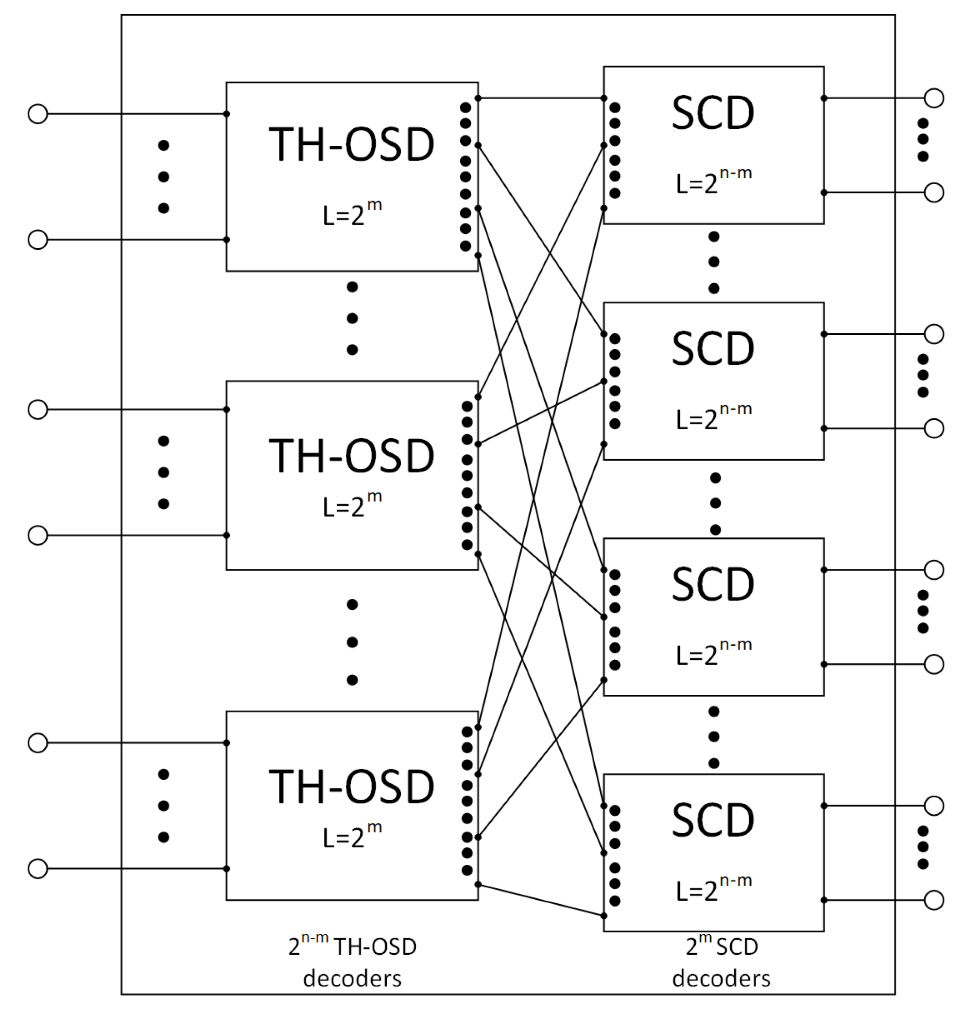
7. Extend to Long Polar Codes

In this section, we describe how to apply TH-OSD to longer polar codes. Direct use of TH-OSD on long codes is not practical since the number of possible codewords grows too fast. Li et al. [16] decomposed the overall polar code into an inner code and an outer code. We can apply TH-OSD as the decoder of the outer code and SC as the decoder of the inner code. Figure 2 shows the structure of the hybrid TH-OSD-SC decoding algorithm. We should restrict the length of the outer code (e.g., 64, 128, and 256) in order to apply TH-OSD. Based on the analysis in Section 5, we conclude that this hybrid decoding algorithm provides lower WER and faster decoding speed than SC dose.

8. Simulation Results

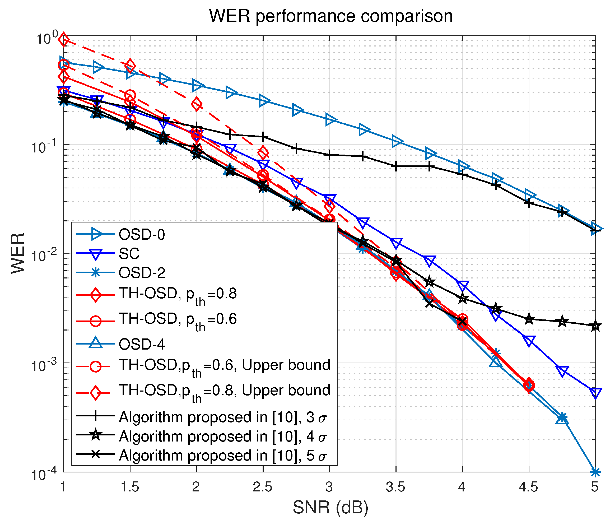
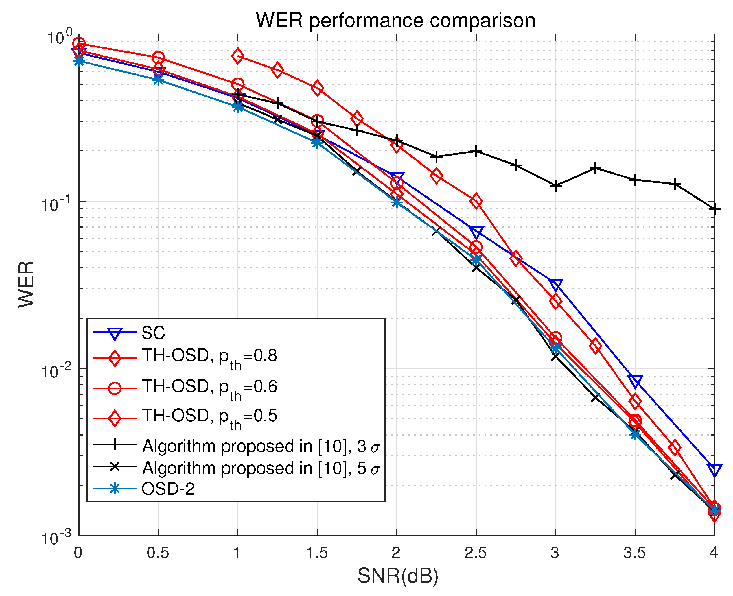
8.1. WER Performance

In this section, we show some simulation results of our proposed algorithm. We tested the WER performance of the proposed decoding algorithm on (64,32) and (128,64) polar codes over a BIAWGN channel and have made other comparisons with the SC, OSD, and SCL decoding algorithm with various list sizes. Figure 3 and Figure 4 plot the WER performance of the decoding algorithms along with the upper-bound computed using Equation (9) with different threshold settings.
As the figures show, the OSD algorithm performed the best among all the algorithms with TH-OSD’s WER performance below that of OSD. However, as the threshold decreased, TH-OSD’s WER performance approached OSD’s. The performance of OSD-4 was the same as OSD-2’s. These observations are in line with our expectations and confirm that OSD-2 performs similarly to MLD in short-code length scenarios. TH-OSD tested fewer candidate codewords compared to OSD. With a high threshold, TH-OSD performed similarly to SC with low SNR values and outperformed it with mid-to-high SNR values. As the threshold is decreased, TH-OSD’s performance improved at the price of testing more codewords. The performance of the proposed algorithm in [10] with threshold 3 σ is rather poor, and the performance with threshold 5 σ is close to OSD-2’s performance at the price of barely no complexity reduction compared to the original OSD which can be seen in the next subsection. The SC is a suboptimal decoding method since it discards the information provided by further frozen bits when decoding an information bit [4]. As a result, SC’s WER performance was not good. SCL with a large list size also achieved performance similar to MLD’s, but we excluded its curve from Figure 3 to preserve clarity.
Figure 3 and Figure 4 also show a noticeable gap between the trajectories of TH-OSD and OSD in low SNR areas. The gap between TH-OSD and OSD was larger with higher threshold settings since a codeword with a higher f value is less likely to be the transmitted codeword. One way to reduce this gap is to use a list. By using a list, a candidate codeword with an f value less than the threshold will not be declared immediately as the decoded codeword. Instead, we put the codeword in the candidate list if the list is not full. We terminate the decoding process once the candidate list is full and declare the candidate codeword with the smallest f value as the decoded codeword. By simulation, we found that a list of size 2 is enough to pull TH-OSD’s trajectory towards OSD’s. Figure 5 shows the effects of a size 2 list: TH-OSD’s WER performance was almost the same as OSD-2’s. Figure 5 also shows the performance of CA-OSD and CA-TH-OSD. We simulated length 64 polar code with 4-bit CRC whose generator polynomial is g ( x ) = x 4 + x + 1 . Figure 5 shows the two crc-aided algorithms both outperformed OSD-2. Thus, they also outperformed MLD since OSD-2 performed maximum likelihood decoding in this scenario. CA-TH-OSD performed almost the same as CA-OSD but tested fewer codewords.

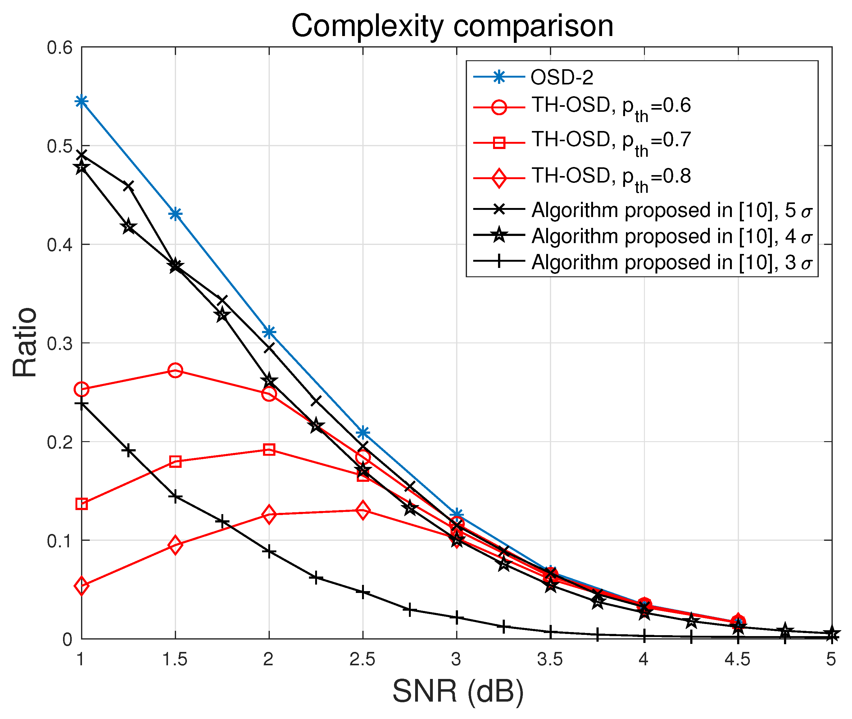
8.2. Complexity Performance

We have also compared the speed of OSD, the algorithm proposed in [10] and TH-OSD by counting the number of codewords tested during the decoding process. Figure 6 shows the proportion of the number of tested codewords compared to the number of all possible codewords during the decoding process of a (64, 32) polar code over a BIAWGN channel using OSD and TH-OSD decoding algorithms. We simulated each algorithm 1,000,000 times for a given SNR range. The figure shows that setting a threshold resulted in TH-OSD testing fewer codewords than OSD did, leading to less decoding time. This reduction was considerable in low SNR situations with acceptable WER performance loss. For example, by setting p t h to 0.8, TH-OSD tested 5% of the total possible codewords, on average, while OSD tested 55% with an SNR of 1 dB. Even setting p t h to 0.6, which resulted in a similar WER compared to OSD, TH-OSD still tested about 50% fewer codewords than OSD for a low SNR. Figure 6 also includes the complexity performance of the proposed algorithm in [10]. Although by setting threshold to 3 σ resulted in significant reduction of tested codewords, the WER performance was unsatisfactory, which can be seen in Figure 3. To achieve near MLD WER using the algorithm proposed in [10], we needed to set threshold to 4 σ or even higher, which led to fairly small reduction of the tested codewords compared to original OSD. Table 2 shows the numerical results of the reduction in tested codewords between the two methods. We also noticed that, in high SNR areas, OSD and TH-OSD were faster than SC in the simulations. This is partly because OSD and TH-OSD both terminate after testing only a few codewords. Additionally, the Gaussian elimination operations during RREF process are simple binary additions, while SC uses expensive hyperbolic function calculations. Although this comparison is not rigorous, it is consistent with our analysis.
In summary, with appropriate threshold settings, TH-OSD increases the decoding speed of OSD while maintaining similar WER performance. TH-OSD is faster than SC when the SNR is high. We also conclude that TH-OSD is faster than SCL with large list sizes because SCL with a list size of L runs 1 / L as fast as SC, which is already slower than TH-OSD.

9. Conclusions

In this paper, we propose a threshold-based flexible OSD decoding algorithm to reduce the complexity of the OSD algorithm while maintaining an acceptable WER under various thresholds of short polar codes. Compared with other decoding algorithms, our proposed TH-OSD algorithm shows better WER performance than SC and runs faster than the OSD algorithm with negligible WER performance loss with appropriate threshold settings. We also provide a method for determining an appropriate threshold value and derive an upper-bound on the WER performance of the proposed TH-OSD algorithm. We implement a list approach to improve the WER performance of TH-OSD to a near MLD performance. A CRC-aided TH-OSD algorithm is also presented, which outperforms MLD. The TH-OSD can be easily extended to longer codes using the structure provided by Li et al. [16]. In the future, we plan to simplify further the expression for the upper-bound of WER performance.

Author Contributions

Conceptualization, Y.X.; methodology, Y.X. and G.T.; formal analysis, Y.X.; Investigation, Y.X.; writing—original draft preparation, Y.X.; writing—review and editing, Y.X. and G.T.; Supervision, G.T.; and Funding acquisition, G.T.

Funding

This work was supported by the National Natural Science Foundation of China (Grant Nos. 61571416 and 61271282) and the Award Foundation of Chinese Academy of Sciences (Grant No. 2017-6-17).

Acknowledgments

We thank LetPub (www.letpub.com) for its linguistic assistance during the preparation of this manuscript.

Conflicts of Interest

The authors declare no conflict of interest.

Appendix A

Appendix A.1. The Mean of the Random Variable r Defined in Equation (4)

Using the relationship defined in Equation (4), we obtain
E ( r ) = 0 y f Y ( y ) d y = 0 y 1 2 π σ e ( y 1 ) 2 2 σ 2 d y = 1 σ ( σ t + 1 ) 1 2 π e t 2 2 d t = 1 σ 1 2 π e t 2 2 d t σ 1 σ 1 2 π e t 2 2 t d t = Q 1 σ + σ 2 π e 1 2 σ 2
where Q ( x ) is the tail probability of the standard normal distribution N ( 0 , 1 ) .

Appendix A.2. The Variance of the Random Variable r Defined in Equation (4)

To obtain the variance of r, we first derive E ( r 2 ) :
E ( r 2 ) = 0 y 2 1 2 π σ e ( y 1 ) 2 2 σ 2 d y = 1 σ ( σ t + 1 ) 2 1 2 π e t 2 2 d t = 1 σ ( σ 2 t 2 + 2 σ t + 1 ) 1 2 π e t 2 2 d t = σ 2 π e t 2 2 + σ 2 Q 1 σ + 2 σ 2 π e t 2 2 + Q 1 σ = ( 1 + σ 2 ) Q 1 σ σ 2 π e 1 2 σ 2
Since the variance of a random variable equals the expectation of the square of this random variable minus the square of the expectation of this random variable, we obtain
Var ( r ) = E ( r 2 ) E ( r ) 2 = ( 1 + σ 2 ) Q 1 σ σ 2 π e 1 2 σ 2 Q 1 σ + σ 2 π e 1 2 σ 2 2

Appendix B. Upper-Bound on the Gap

In the following derivations, we assume that an all-zero codeword is sent and that y 1 , y 2 , , y N denotes the received vector. We begin with the gap and make progressive simplifications.
P G a p ( f t h ) Pr 0 = arg min C L c f ( C ) , | N M R I P | i , C 0 , f ( C ) f t h , C is met before 0 Pr 0 = arg min C L c f ( C ) , | N M R I P | i , C 0 , f ( C ) f t h = d = 0 N K d H + 1 P D ( d ) Pr | N M R I P | i , C 0 , f ( C ) f t h | D = d = d = 0 N K d H + 1 P D ( d ) A ( d , f t h )
where | N M R I P | denotes the number of negative values in the MRIPs, and d H is the minimum codeword weight. K + d is the index of the last MRIP. L c is the candidate codeword list.
A ( d , f t h ) can be expressed and further bounded as follows:
A ( d , f t h ) = Pr | N M R I P | i , C 0 , f ( C ) f t h | D = d j = 1 i K j Pr | N M R I P | = j , C 0 , f ( C ) f t h | D = d = j = 1 i K j 0 f t h Pr | N M R I P | = j , C 0 , f ( C ) f t h , y K + d = x | D = d d x = j = 1 i K j 0 f t h B j , d ( x ) d x
We used union bound in the second step in Equation (A5). B j , d ( x ) is the probability density function of the event that a codeword chosen from the candidate list has a discrepancy less than f t h while j out of the K MRIPs are negative and the ( K + d ) th received value is x.
B j , d ( x ) can be further bounded by the following equations:
B j , d ( x ) N ! ( K + d 1 ) ! ( N K d ) ! T ( x ) K + d 1 1 T ( x ) j 1 F | y | ( x ) K + d 1 · F | y | ( x ) N K d 1 2 π σ e x 1 2 2 σ 2 G σ , f t h ( x )
where T ( x ) represents the probability that a Gaussian random variable y N ( 1 , σ 2 ) is positive under the condition | y | x ; F | y | is the CDF of random variable | y | ; and G σ , f t h ( x ) represents the probability that a codeword has a discrepancy less than f t h under the condition y + K + d = x and j out of the K MRIPs are negative. Since the non-zero codeword we considered here flips at least one MRIP, and its weight is at least d H , G σ , f t h ( x ) can be approximately bounded by
G σ , f t h ( x ) Q μ ( x ) f t h + x σ ( x )
where μ ( x ) and σ ( x ) are the mean and variance of the portion of the discrepancy of a codeword C (C has one “1” in the first ( K + d ) positions and ( d H 1 ) “1”s in the remaining ( N K d ) positions) contributed by the last ( N K d ) positions. Expressions of μ ( x ) and σ ( x ) are as follows:
μ ( x ) = N K d d H + 1 μ n ( x ) + d H 1 μ p ( x )
σ ( x ) 2 = N K d d H + 1 σ n 2 ( x ) + d H 1 σ p 2 ( x )
where in the preceding, μ n ( x ) , μ p ( x ) , σ n 2 ( x ) and σ p 2 ( x ) can be calculated using the following equations:
μ n ( x ) = x 0 s x ( t ) ( t ) d t
μ p ( x ) = 0 x s x ( t ) t d t
σ n 2 ( x ) = x 0 s x ( t ) t + μ n ( x ) 2 d t + μ n 2 ( x ) 0 x s x ( t ) d t
σ p 2 ( x ) = 0 x s x ( t ) t μ p ( x ) 2 d t + μ p 2 ( x ) x 0 s x ( t ) d t
where s ( · ) is the probability density function of a random variable y N ( 1 , σ 2 ) under the condition | y | x .

Appendix C. Complexity Analysis of the SC Decoding Algorithm

In this section, we analyze the number of different operations (e.g., tanh and atanh) required by the LLR-based SC decoding algorithm. The SC decoding algorithm is a recursive algorithm with the following complexity:
T ( N ) = 2 T N 2 + t ( N )
where T ( N ) is the number of operations needed for decoding a length-N sequence, and t ( N ) is the number of operations needed for preparing data for sub-problems (the merging step). The merging step performs N tanh operations, N 2 atanh operations, N 2 float additions, and N 2 float multiplications [4]. Thus, t ( N ) = 5 2 N , and Equation (A14) turns into
T ( N ) = 2 T N 2 + 5 N 2
Solving Equation (A15), we obtain T ( N ) = 5 2 N log N . These operations are composed of N log N tanh operations, 1 2 N log N atanh operations, 1 2 N log N multiplications, and 1 2 N log N additions.

References

  1. Arikan, E. A method for constructing capacity-achieving codes for symmetric binary-input memoryless channels. IEEE Trans. Inf. Theory 2009, 55, 3051–3073. [Google Scholar] [CrossRef]
  2. Tal, I.; Vardy, A. List decoding of polar codes. ISIT 2011. [Google Scholar] [CrossRef]
  3. Niu, K.; Chen, K. Stack decoding of polar codes. Electron. Lett. 2012, 48, 695–697. [Google Scholar] [CrossRef]
  4. Balatsoukas-Stimming, A.; Parizi, M.B.; Burg, A. LLR-based successive cancellation list decoding of polar codes. ICASSP 2014. [Google Scholar] [CrossRef]
  5. Niu, K.; Chen, K. CRC-aided decoding of polar codes. IEEE Commun. Lett. 2012, 16, 1668–1671. [Google Scholar] [CrossRef]
  6. Kaneko, T.; Nishijima, T.; Inazumi, H.; Hirasawa, S. An efficient maximum-likelihood-decoding algorithm for linear block codes with algebraic decoder. IEEE Trans. Inf. Theory 1994, 40, 320–327. [Google Scholar] [CrossRef]
  7. Kaneko, T.; Nishijima, T.; Hirasawa, S. An improvement of soft-decision maximum-likelihood decoding algorithm using hard-decision bounded-distance decoding. IEEE Trans. Inf. Theory 1997, 43, 1314–1319. [Google Scholar] [CrossRef]
  8. Wu, X.; Sadjadpour, H.R.; Tian, Z. A new adaptive two-stage maximum-likelihood decoding algorithm for linear block codes. IEEE Trans. Commun. 2005, 53, 909–913. [Google Scholar] [CrossRef]
  9. Kahraman, S.; Çelebi, M.E. Code based efficient maximum-likelihood decoding of short polar codes. ISIT 2012, 1967–1971. [Google Scholar] [CrossRef]
  10. Wu, D.; Li, Y.; Guo, X.; Sun, Y. Ordered statistic decoding for short polar codes. IEEE Commun. Lett. 2016, 20, 1064–1067. [Google Scholar] [CrossRef]
  11. Fossorier, M.P.; Lin, S. Soft-decision decoding of linear block codes based on ordered statistics. IEEE Trans. Inf. Theory 1995, 41, 1379–1396. [Google Scholar] [CrossRef] [Green Version]
  12. Trifonov, P. Efficient design and decoding of polar codes. IEEE Trans. Commun. 2012, 60, 3221–3227. [Google Scholar] [CrossRef]
  13. Lin, S.; Costello, D.J. Error Control Coding, 2nd ed.; Prentice-Hall, Inc.: Upper Saddle River, NJ, USA, 2004. [Google Scholar]
  14. Hussami, N.; Korada, S.B.; Urbanke, R. Performance of polar codes for channel and source coding. ISIT 2009, 1488–1492. [Google Scholar] [CrossRef]
  15. Papoulis, A.; Pillai, S.U. Probability, Random Variables, and Stochastic Processes; McGraw-Hill Higher Education: New York, NY, USA, 2002. [Google Scholar]
  16. Li, B.; Shen, H.; Tse, D.; Tong, W. Low-latency polar codes via hybrid decoding. ISTC 2014, 223–227. [Google Scholar] [CrossRef]
Figure 1. The empirical CDF of f and the Gaussian approximation for different SNR values with codeword length N = 64 .
Applsci 09 00831 g001
Figure 2. The structure of hybrid TH-OSD-SC decoding algorithm.
Applsci 09 00831 g002
Figure 3. WER performance comparison between SC, OSD, the algorithm proposed in [10] and TH-OSD with codeword length 64 and rate 0.5.
Applsci 09 00831 g003
Figure 4. WER performance comparison between SC, OSD, the algorithm proposed in [10] and TH-OSD with codeword length 128 and rate 0.5.
Applsci 09 00831 g004
Figure 5. WER performance comparison between OSD-2, TH-OSD, TH-OSD list, CA-OSD, and CA-TH-OSD.
Applsci 09 00831 g005
Figure 6. Comparison of total tested codewords of OSD-2, the algorithm proposed in [10] and TH-OSD-2 with different threshold settings, code length 64, and rate 0.5.
Applsci 09 00831 g006
Table 1. Threshold values when p t h = 0.7 and codeword length N = 64 .
SNR(dB)11.522.533.544.5
f t h 5.15734.18013.35122.65432.07431.59711.20960.8995
Table 2. Reduction in the number of tested codewords compared to OSD (Codeword length 64 and rate 1/2).
SNR(dB) p t h = 0.6 p t h = 0.7 p t h = 0.8
153.6%74.9%90.1%
1.536.8%58.3%78.0%
220.1%38.3%59.5%
2.511.9%20.9%37.6%
37.5%12.3%19.0%
3.54.2%6.9%11.0%

