Abstract
The development of high-speed camera systems and image processing techniques has promoted the use of vision-based methods as a practical alternative for the analysis of non-contact structural dynamic responses. In this study, a deviation extraction method is introduced to obtain deviation signals from structural idealized edge profiles. Given that the deviation temporal variations can reflect the structural vibration characteristics, a method based on singular-value decomposition (SVD) is proposed to extract valuable vibration signals from the matrix composed of deviations from all video frames. However, this method exhibits limitations when handling low-level motions that reflect high-frequency vibration components. Hence, a video acceleration magnification algorithm is employed to enhance low-level deviation variations before the extraction. The enhancement of low-level deviation variations is validated by a light-weight cantilever beam experiment and a noise barrier field test. From the extracted waveforms and their spectrums from the original and magnified videos, subtle deviations of the selected straight-line edge profiles are magnified in the reconstructed videos, and low-level high-frequency vibration signals are successfully enhanced in the final extraction results. Vibration characteristics of the test beam and the noise barrier are then analyzed using signals obtained by the proposed method.
1. Introduction
The dynamic responses of structures with complex configurations, such as mechanical equipment, bridges, and buildings, are typically measured using a set of mounted transducers, such as accelerometers and strain gauges. The development of high-speed camera systems and image-processing techniques has promoted the use of vision-based measurement in the study of structural health monitoring [1,2,3], dynamics modal analysis [4,5,6], and nondestructive testing [7,8,9]. In contrast with traditional contact sensors, vision-based methods provide an intuitionistic demonstration of actual structural vibration and are more convenient for installation under conditions where contact sensors have difficult access. Without additional mass on the surface of the measurement target, vision-based measurement devices rarely affect the natural properties of flexible or lightweight objects. Moreover, vision-based devices often have a flexible composition and provide relatively high spatial resolution in an efficient and automated manner [10].
The emergence of high-speed imaging sensors allows the camera to work at a high sampling rate with considerable resolution in the film. Structural high-frequency motions can be recorded in a high-speed video file, and noises from frame interpolation are technically avoided in subsequent image processing. Valuable motion signals hidden in video frames can be extracted by combining image processing algorithms, such as optical flow [11,12] and image correlation [13,14] (including digital image correlation (DIC)). Therefore, motion estimation from a sequence of video has become a popular problem in the computer vision field. High-speed video cameras have potential applications and have been successfully used for experimental modal analysis [15,16], sound information recovery [17,18,19], and fault diagnosis [20,21].
Traditional image template matching algorithms calculate cross-correlation parameters between the selected template subimage and subimages in the following video frames and locate the best matching pixel coordinates [22,23,24]. However, the cross-correlation function may be valid when facing poor and repetitive textures. The deviations of structural idealized edge profiles can be employed to extract effective motion signals. This method is simplified from a deviation magnification (DM) algorithm [25] without the magnification and image reconstruction processes. In contrast to intensity- and phase-based optical flow [11,26], which calculate the relative spatial and temporal derivative field by solving the aperture equation at each pixel between consecutive frames, the deviation extraction algorithm reveals geometric deviations from their idealized edge profiles (e.g., straight-line and curves) in a single image. With all deviations from a selected contour extracted, the global variations in these signals can be applied to analyze structural vibration characteristics.
The variations in deviations are sensitive to structural low-frequency vibration, which has a relatively large amplitude. However, this method exhibits limitations when handling low-level motions on the idealized edge profile that reflect high-frequency components. In this regard, the Eulerian video magnification (EVM) algorithm [27,28,29] is introduced to preprocess subtle high-frequency vibrations in video before deviation extraction. Subtle motions and deviations in video are usually difficult to perceive with the human eye without any image processing. The core concept of motion magnification is to allow subtle variations in a specific frequency band to be observed intuitively by magnifying small intensity or phase variations in the video. Compared with intensity-based video magnification [27], the magnification of phase will not be restrained by the imitation of the pixel value and has better control of additional image noise. Therefore, phase-based video magnification can be used to enhance the low-level variations of the selected edge profile.
Linear phase-based motion magnification fails for moving objects because large motions overwhelm small temporal variations. In practical measurement, only low-level small variations are magnified rather than large motions, such as object motion or the camera. For this reason, an acceleration motion magnification is employed to handle high-speed video before deviation extraction [30]. The image signal is first separated into multi-frequency bands and orientations by the complex steerable pyramid. By assuming that the large motion is approximately linear at the temporal scale of the small change, a second-order temporal derivative filter is used to calculate non-linear phase acceleration variations of video frames. Compared with that in the linear-based approach, the video after acceleration magnification has better control over image blurring and artifacts so that the structural contour is less influenced by the magnification. Subtle low-level deviation on the idealized edge profile can be effectively enhanced in the magnified high-speed video.
This study proposes an approach for extracting the low-level valuable vibration signal from deviations of the structural idealized edge profile. The video acceleration magnification algorithm is applied to enhance subtle low-level variations along the selected contour. The deviations of the idealized edge profile in all video frames are then extracted and used to reconstruct an analysis matrix. Given that the relative intensity variations along the structural edge profile reflect their vibration characteristics, a method based on singular-value decomposition (SVD) is introduced to extract useful vibration signals involved in the analysis matrix. Without the requirement of textures on the target, our approach handles intensity variations that are vertical to straight-line or curve edges, and subtle structural vibration signals can be extracted from another perspective.
The rest of the paper is organized as follows. The theoretical part first discusses derivations of the deviation extraction algorithm. An experiment on a saw blade is conducted to illustrate the specific deviation extraction. The video acceleration magnification algorithm for enhancing low-level subtle variations is then introduced in the following subsection. A simple black circle simulation test is given to show the effect of motion magnification. The SVD-based vibration extraction approach is presented to extract valuable variation signals from the generated analysis matrix. Two experiments are conducted in the verification part to demonstrate the practical effect of the video acceleration magnification and SVD-based extraction. The low-level dynamic responses of a clamped cantilever beam and a noise barrier are analyzed thoroughly by using the proposed method and high-speed camera systems. The discussion and conclusions are presented in the final section.
2. Theory and Algorithm
2.1. Deviation Extraction in a Single Image
Structural deviation variations should be extracted from video frames at the beginning of the analysis process. Consider a simple idealized edge profile in subimage , where is the pixel coordinate and refers to the timeline; the edge profile at location x can be defined as:
Assuming that subtle deviation variations exist at every location x along the edge profile, the edge profile signal can be approximated as follows:
As the deviation variation is considered to be subtle, the edge profile signal can be approximated using the mean or median value of all available intensities along the y direction. Thus, is expressed as:
where represents the independent image noise in every pixel coordinate. This equation is expanded with first-order Taylor approximation with nonlinear components ignored:
Therefore, the mean value over x is computed as:
where N is the number of pixels along the x axis. It is seen that the remaining noise term is an item only of parameter y and has less variance than the original . Given that is small and is also extremely small, another Taylor expansion leads to:
As can be seen from the derivations above, the average edge profile approximates the common edge profile up to a constant shift item. Given the observations of , deviation signal can be obtained by using a least squares estimation:
which leads to the final approximate solution of the deviation variations in single subimage :
We demonstrated the effectiveness of the deviation extraction by using a simple carbon tool steel saw blade experiment. A saw blade has a jagged edge on one side and a smooth edge on the other side. Figure 1a shows the tested saw blade fixed on a table vice. The image was captured with a Canon 70D SLR camera, and the shapes of the jagged edge and the smooth edge are difficult to identify with the naked human eye in the original image. Common edge detection algorithms will identify the jagged edge as an idealized straight-line element. These ideal geometries such as straight-line or curves on the surface of the test structure are considered to be the idealized edge profiles [25]. Our ultimate target is to extract subtle deviation variations along the jagged edge and the smooth edge. In this experiment, an analysis area was selected in Figure 1a for further operations.
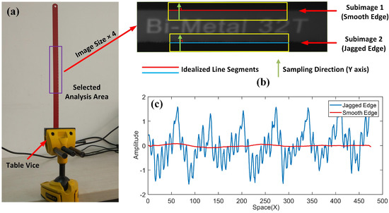
Figure 1.
Experimental setups of the saw blade experiment: (a) saw blade and the selected analysis area; (b,c) schematic and extraction results of the saw blade experiment.
The selected analysis area is transformed from the RGB color space to grayscale because the deviation extraction algorithm only works on image intensities. From Figure 1b, two subimages within the yellow rectangles are selected as the regions of interest (ROIs). The size of the ROIs is 480 × 50 pixels, and the red and blue lines within the ROIs represent the idealized straight-line segments that are identified using the line segment detector. In reality, these detected line elements are not perfectly straight-lines and contain unnoticeable subtle vibrations. During the analysis, the detected smooth and jagged sides are considered as idealized straight-lines for the convenience of the following sampling process. We consider the direction of the idealized straight-line segments as the x axis, and the edge profiles are then sampled strictly perpendicular to it. The sampling direction (y axis) is marked with green arrows in Figure 1b. Figure 1c shows the output deviation extraction signals of the jagged edge and the smooth edge without performing any denoising process. The unnoticeable cyclical jagged shape marked with a blue line is extracted successfully from the saw blade subimage. The amplitude of the deviation signal on the smooth side is quite small (less than 0.1) and can be observed as a smooth line.
The simple saw blade experiment above explains the deviation extraction process from the idealized straight-line profiles. The sampling directions are programmed to be strictly perpendicular to the identified line to observe variations that are vertical to the idealized straight lines. For complicated edge profiles, such as circular or ellipse boundaries, the idealized fitted curves can be calculated by edge extraction methods, such as Hough transformation. Polar coordinates instead of rectangular coordinates are applied to locate the sampled pixel intensities. Given a high-speed video file containing M frames, we consider the deviation differences between the first frame and the frame as the global edge translation signal.
2.2. Low-Level Variation Magnification
In practical measurement, lower frequency structural boundary variations commonly have a larger vibration amplitude and will occupy more energy of the global edge translation signals. By contrast, low-level high-frequency variations of the detected edge profile may be covered by the noise, which makes these signals difficult to extract. To enhance these low-level components, we use phase-based Eulerian video magnification (PEVM) to preprocess subtle changes in video before the deviation extraction.
In contrast to the intensity-based linear video magnification method [27], which handles the pixel values of the image sequence independently in the time line, PEVM visualizes subtle motions in video by band-pass filtering of temporal image phases. Variations in specific frequency bands can be magnified and visualized in the reconstructed video. Considering that linear temporal phase variations are sensitive to large motions, such as camera or object motion, we follow the acceleration magnification method of Zhang et al.
For a 1D signal at positon x and time t, linear methods [27,28,29] assume a displacement function such that . The magnified counterpart of is defined as:
The second-order Taylor expansion yields:
By assuming that the large object motion is approximately linear, the band-pass filtering and magnification processes will be conducted on the second-order non-linear item:
The reconstructed magnified signal can be calculated as:
where is the amplification factor. The difference between linear and acceleration magnification in the 1D signal is illustrated in Figure 2. The red lines show the signal magnification results for factor . The purple curves show the magnified linear and acceleration variations of the 1D signal. Compared with the linear method, acceleration magnification handles only small motion and is more robust to large translational motions.
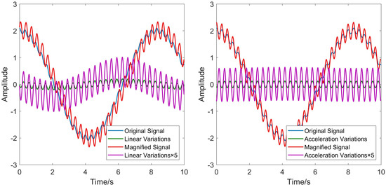
Figure 2.
Comparisons between linear motion magnification and acceleration magnification [30].
Motion can be represented by a phase shift; as such, phase-based acceleration magnification operates on the second-order temporal phase variations of the image sequence. For a given image in timeline t, the complex steerable pyramid [31] decomposes the image signal into multiple frequency bands at scale and orientation :
where ⊗ is convolution, is the temporal amplitude, and is the temporal phase. The second-order derivative of the Gaussian filter , namely the Laplacian filter, is applied to extract subtle phase variations of interest [32,33]:
where is the temporal Laplacian filter with the kernel as . The parameter r is the frame rate, and is the target frequency. Therefore, the magnified phase with amplification factor is given by:
Eventually, the reconstructed magnified image can be calculated by using the image amplitude and the magnified phase.
A simulation test is provided to illustrate the acceleration magnification result. From Figure 3a, a simple vignetting black circle, which has a diameter of 240 pixels, is programmed to vibrate in a sinusoidal manner with 0.2-pixel amplitude in the vertical direction. Figure 3c shows the magnified video image. Based on the comparison between the pixel time slices marked with red lines in Figure 3a,c, subtle vibration is successfully magnified in the reconstructed video file. In pixel time slices, the horizontal axis is the frame number, and the vertical axis is the intensity values cut from the red line in the corresponding frame. Figure 3b shows the polluted black circle video that contains Gaussian white noise with variance 0.005, and the magnified result is given in Figure 3d. Benefiting from the temporal filtering process, noise in the reconstructed video frame is significantly reduced.
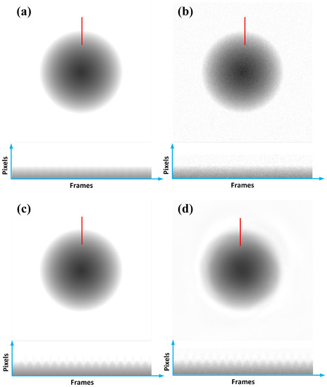
Figure 3.
The black circle simulation test: (a) original clean video frame and pixel time slice; (b) noise video frame with Gaussian white noise of variance 0.005 and pixel time slice; (c) magnified clean video frame and pixel time slice; (d) magnified noise video frame and pixel time slice.
2.3. SVD-Based Variations’ Extraction
Acceleration video magnification enhances the energy of the lower-level structural boundary variations. Therefore, the deviations can be extracted from idealized edge profiles in the magnified video frames. With all global edge translation signals in ROIs calculated from the magnified video with Equation (8), these signals are employed to construct an analysis matrix that is formed with subtle variations of the idealized edge profile:
where M is the number of images in the video, N is the sampling pixel number along the x axis and sign ∗ represents the matrix transposition. In order to extract a valuable structural vibration signal from the matrix , a singular-value decomposition (SVD)-based approach is employed.
As a factorization method of the matrix in linear algebra, the SVD is broadly applied in signal denoising and data compression areas. For a given real matrix , the SVD decomposes the matrix of the form:
where is a diagonal matrix with non-negative singular values on the diagonal in descending order, and are both unitary matrices composed of orthonormal eigenvectors, and matrix represents the conjugate transpose of matrix .
It is known that the magnitude of the singular values in matrix indicates the energy distribution of vibration signals and noise. Since the magnitude of the singular values corresponding to noise are relatively lower, the available vibration signal can be calculated by using the low-rank approximation of the matrix according to the Eckart–Young theorem:
where are the former k singular values and the other singular values are all replaced by zero. In practical applications, we use the column summation of matrix to further study vibration characteristics. In summary, the overall flowchart of our proposed vibration extraction process is shown in Figure 4. For textured edge profiles that may introduce noise to the deviation extraction result, we follow the image coloration optimization method of Levin et al.

Figure 4.
Flowchart of the low-level variation magnification and extraction process.
During the deviation extraction, every deviation variation contains a random constant shift of , which reflects a constant shift [25]. In contrast to optical flow or image registration motion extraction algorithms, which calculate the true displacement value, signals extracted using the SVD-based method only reflect the tendency of the structure’s vibration. It should be noted that all extracted vibration signals in the following experiments are normalized signals extracted by the SVD-based approach. Nevertheless, these signals remain acceptable and have a high cross-correlation relationship with true vibrations [18].
3. Experimental Verifications
3.1. Light-Weight Beam Property Analysis
A laboratory experiment on the saw blade in Figure 1 was carried out to evaluate the effectiveness of the proposed method. The experimental setup is shown in Figure 5. The saw blade in Figure 1 was clamped with a table vice and can be approximately considered as a light-weight cantilever beam. The dimensions of the test beam is 0.29 m × 0.0126 m × 0.00065 m. The Young’s modulus of the material is 2.06 × 10 N·m, and the density is 7.85 × 10 kg·m. An audio file with frequency band from 10 Hz–500 Hz was played by a loudspeaker from approximately 0.1 m away from the target to excite the beam. The sound volume was set to 80 dB. Air fluctuations can induce subtle vibration on the surface of the cantilever beam. These vibrations were captured with the high-speed camera system (Mode-5KF10M, Agile Device Inc., Hefei, China) at 500 fps with a resolution of 580 × 180 pixels. An LED light source was used to ensure environmental illumination because the exposure time of the high-speed camera is short and ambient light cannot provide adequate illumination.
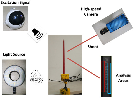
Figure 5.
Setups of the beam property estimation experiment.
The captured video file was first handled by the phase-based acceleration magnification algorithm. Laplacian kernels in motion magnification were calculated according to the theoretical resonant frequencies that were obtained by using Euler–Bernoulli beam theory. Two subimage areas were then selected within the red (the jagged side) and blue (the smooth side) rectangles to extract deviation signals. The size of the selected two subimages was 300 × 30 pixels. The analysis matrix can be generated with deviation variation signals in all frames calculated. The SVD results indicate that the signals corresponding to the first two singular values took over 90% of the energy in the obtained analysis matrix. The rest of the components in the analysis matrix were considered to be noise and ignored in the low-rank approximation matrix. The waveforms and frequency spectrums of the vibration signals from the smooth side and jagged side of the saw blade are shown in Figure 6 and Figure 7.
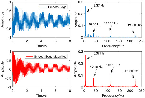
Figure 6.
Vibration signals and their frequency spectrums extracted from the original video (blue line) and the magnified video (red line) along the smooth edge of the saw blade.
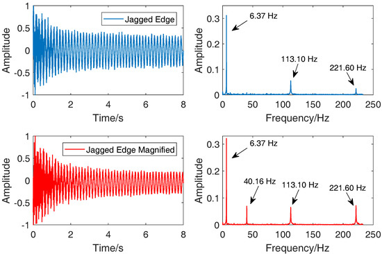
Figure 7.
Vibration signals and their frequency spectrums extracted from the original video (blue line) and the magnified video (red line) along the jagged edge of the saw blade.
From the following spectra, four obvious peaks for 6.37 Hz, 40.16 Hz, 113.10 Hz, and 221.60 Hz were found using the magnified video file. The edge variations corresponding to these four peaks were not extracted effectively from the original video. The peak for 40.16 Hz was difficult to find in the vibration signal from the original jagged edge. The low-level vibration signals over 40 Hz were successfully magnified in the video processed by acceleration magnification. Table 1 shows the first four resonant frequencies estimated according to the classical Euler–Bernoulli beam theory. These four peaks match well with the theoretical ones. Given that the vibration signal of the first-order resonant frequency is clear, the magnification was not applied to the first-order resonant frequency. The Laplacian kernels and video magnification factors are given in Table 1.

Table 1.
Identified modal frequencies and analysis parameters in the beam test.
In practical applications, the experimental modal frequencies can help estimate structural vibration properties, such as elasticity. Although acceleration magnification rarely induces image blurring and artifacts, a large amplification factor may induce image motion-blurred images and affect the extraction result. In this particular case, the amplification factors were controlled to less than 15.
3.2. Vibration Analysis of the Noise Barrier
A noise barrier is an exterior structure designed to protect inhabitants of sensitive land use areas from noise pollution. The noise barriers are installed on both sides of the CRHtrain railway bridge to mitigate noise from the railway when a train is passing by. These platy structures usually suffer from strong suction induced by the CRH train under practical working conditions. Wind pressure when a high-speed train passes by can cause harmful vibrations to the noise barriers and decrease the designed service life. Figure 8 shows the experimental setups of the noise barrier vibration test. The field test was conducted near the KunShan railway station, which is an important railway hub in East China. The height of the viaduct is about 12 m, and traditional contact sensors are difficult to install.
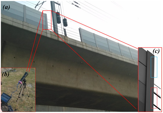
Figure 8.
Noise barrier experiment setups: (a) the experiment environment; (b) experimental setup; (c) image captured by the high-speed camera and selected analysis areas.
Vision-based vibration extraction is considered a suitable alternative to analyze the dynamic responses of the noise barrier when a high-speed train passes by. The high-speed camera (Mode-5KF04M, Agile Device Inc.) was placed below the viaduct at a distance of about 28 m, and the distance between the camera head and the target was set to 30 m. The tilt angle was estimated to be , and the error rate caused by the tilt angle was approximately 0.6%∼0.8% [34]. The filming was begun shortly before the high-speed train arrived. The frame rate of the video was set to 232 fps, and the resolution of the image was 660 × 880 pixels during the experiment. We selected two analysis areas of which the dimensions were 100 × 500 pixels in the video for further vibration analysis. The first smooth area in the blue rectangle is a clean edge without any textures, and the edge in the red rectangle contains visible textures. The colorization optimization algorithm of Levin et al. was employed to remove noise from textures on the boundary before deviation extraction. As shown in Figure 9, the colorization optimization [35] can help remove noise edge variations due to textures and satisfy the constant edge profile assumption.
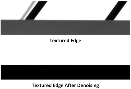
Figure 9.
Selected textured edge and edge after colorization optimization.
The employed Laplacian kernels in motion magnification were calculated by using finite element analysis [36]. The frequency spectra of the extracted waveforms before and after acceleration magnification are compared in Figure 10 and Figure 11. The SVD results indicate that the first two decomposed components took over 92% of the energy in the analysis matrices, so the rest of the singular values were zeroed in the final low-rank approximation signals. The waveforms extracted from the magnified videos contained high-frequency vibrations. Three obvious peaks (10.42 Hz, 21.07 Hz, and 45.77 Hz) were found in the magnified smooth clean edge and the textured edge. Higher order peaks (21.07 Hz and 45.77 Hz) were not clearly found in the signals extracted from the original video files. The used Laplacian kernels and magnification factors are given in Table 2. The results confirm the successful enhancement of low-level vibration signals in the magnified videos.

Figure 10.
Vibration signals extracted from the original video and the magnified video along the smooth clean edge.
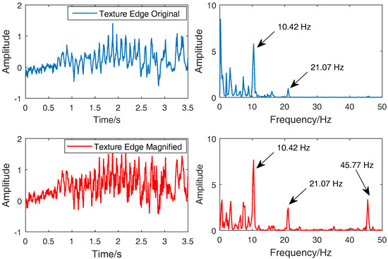
Figure 11.
Vibration signals extracted from the original video and magnified video along the textured edge.
Table 2.
Identified modal frequencies and analysis parameters in the noise barrier experiment.
The natural frequencies of the railway bridge were relatively low and rarely found from train-induced dynamic responses [37,38]. The excitation frequency of the wind load caused by the train carriages was commonly within 2 Hz–4 Hz. The extracted peaks can be considered dominated by excitation associated with the passing of the CRH locomotive train because the arrival of the train can bring strong pulsed wind excitation to the noise barriers [39]. The three peaks are considered to be the natural frequencies of the noise barrier.
There are some issues that should be noted in the field application. Although the acceleration phase-based motion magnification is theoretically more robust to large translational motions, such as camera and object motion, it is recommended to keep the high-speed camera from the large vibration induced by ambient noise. Besides that, an overlarge amplification factor may help to improve the enhancement of low-level variations, and inevitable image noise, and motion blurs in the magnified video may bring errors to the deviation extraction result. In structural high-frequency response measurement, a light source is required to provide adequate illumination during high-speed imaging. Because the deviation extraction algorithm works on the pixel intensities, sudden illumination variations in the field test may lead to unclear edge profiles and influence the final extraction result.
4. Discussion and Conclusions
The deviations of the structural idealized edge profile contain important variations that reflect structural vibration characteristics. Low-level variations along the idealized edge profile are difficult to acquire using the traditional motion extraction method. In this study, an acceleration video magnification algorithm was introduced to magnify low-level edge profile variations in a high-speed video file. The magnified low-level variations were extracted efficiently with an SVD-based motion extraction approach.
The theoretical subsection presented a saw blade experiment to illustrate the deviation extraction process. A simple vignetting black circle simulation test was given to show the influence of motion magnification. Two experiments were conducted in the experimental subsection. Low-level vibrations of a light-weight cantilever beam and a noise barrier were magnified using video magnification. The deviations of the magnified idealized straight-line edge profiles were reconstructed into analysis matrices. Final vibration signals were calculated with the following SVD-based extraction algorithm. From the waveforms and their spectra, low-level high-frequency vibration signals were successfully enhanced in the magnified videos. Vibration characteristics of the test beam and the noise barrier were analyzed using signals obtained by the proposed method.
In contrast to linear phase-based magnification, the acceleration phase-based motion magnification handled only small acceleration vibrations and was more robust to large translational motions; hence, this approach is not sensitive to large motions, such as camera or object motions. However, a large magnification factor will inevitably bring motion blurs to the magnified video and influence the deviation extraction results. Given that the proposed method works on pixel intensities, sudden illumination variations in the video may lead to unclear edge profiles and pollute the deviation of the selected edge profiles. In contrast to optical flow or image registration motion extraction algorithms, which calculate the true displacement value, signals extracted using the SVD-based method only reflect the tendency of the structure’s vibration. Nevertheless, these signals remain acceptable and have a high cross-correlation relationship with true vibrations. Our future work will focus on improving the tolerance of illumination and optimizing the motion blurs under a high magnification factor.
Author Contributions
D.Z., Y.W., and J.G. conceived of and designed the field survey; D.Z., L.F., Y.W., and B.T. carried out the experiments; D.Z. and L.F. processed and analyzed the simulation test and experiment data; D.Z. and L.F. contributed to the methodology and reviewed the submitted manuscript.
Funding
This project was funded by the National Natural Science Foundation of China (No. 51805006 and No. 11802003).
Acknowledgments
The authors would like to thank the anonymous reviewers for their valuable comments and suggestions.
Conflicts of Interest
The authors declare no conflict of interest.
References
- You, D.; Gao, X.; Katayama, S. Monitoring of high-power laser welding using high-speed photographing and image processing. Mech. Syst. Signal Proc. 2014, 49, 39–52. [Google Scholar] [CrossRef]
- Feng, D.; Feng, M.Q. Experimental validation of cost-effective vision-based structural health monitoring. Mech. Syst. Signal Proc. 2017, 88, 199–211. [Google Scholar] [CrossRef]
- Feng, D.; Feng, M.Q. Computer vision for SHM of civil infrastructure: From dynamic response measurement to damage detection—A review. Eng. Struct. 2018, 156, 105–117. [Google Scholar] [CrossRef]
- Poozesh, P.; Sarrafi, A.; Mao, Z.; Avitabile, P.; Niezrecki, C. Feasibility of extracting operating shapes using phase-based motion magnification technique and stereo-photogrammetry. J. Sound Vib. 2017, 407, 350–366. [Google Scholar] [CrossRef]
- Yang, Y.; Dorn, C.; Mancini, T.; Talken, Z.; Nagarajaiah, S.; Kenyon, G.; Farrar, C.; Mascareñas, D. Blind identification of full-field vibration modes of output-only structures from uniformly-sampled, possibly temporally-aliased (sub-Nyquist), video measurements. J. Sound Vib. 2017, 390, 232–256. [Google Scholar] [CrossRef]
- Molina-Viedma, A.J.; Felipe-Sesé, L.; López-Alba, E.; Díaz, F. High frequency mode shapes characterisation using Digital Image Correlation and phase-based motion magnification. Mech. Syst. Signal Proc. 2018, 102, 245–261. [Google Scholar] [CrossRef]
- Park, J.W.; Lee, J.J.; Jung, H.J.; Myung, H. Vision-based displacement measurement method for high-rise building structures using partitioning approach. NDT E Int. 2010, 43, 642–647. [Google Scholar] [CrossRef]
- Cha, Y.J.; Chen, J.G.; Büyüköztürk, O. Output-only computer vision based damage detection using phase-based optical flow and unscented Kalman filters. Eng. Struct. 2017, 132, 300–313. [Google Scholar] [CrossRef]
- Sarrafi, A.; Mao, Z.; Niezrecki, C.; Poozesh, P. Vibration-based damage detection in wind turbine blades using Phase-based Motion Estimation and motion magnification. J. Sound Vib. 2018, 421, 300–318. [Google Scholar] [CrossRef]
- Reu, P.L.; Rohe, D.P.; Jacobs, L.D. Comparison of DIC and LDV for practical vibration and modal measurements. Mech. Syst. Signal Proc. 2017, 86, 2–16. [Google Scholar] [CrossRef]
- Baker, S.; Matthews, I. Lucas-kanade 20 years on: A unifying framework. Int. J. Comput. Vis. 2004, 56, 221–255. [Google Scholar] [CrossRef]
- Guo, J.; Zhu, C.A.; Lu, S.; Zhang, D.; Zhang, C. Vision-based measurement for rotational speed by improving Lucas–Kanade template tracking algorithm. Appl. Opt. 2016, 55, 7186–7194. [Google Scholar] [CrossRef] [PubMed]
- Pan, B.; Tian, L. Superfast robust digital image correlation analysis with parallel computing. Opt. Eng. 2017, 54, 034106. [Google Scholar] [CrossRef]
- Feng, W.; Jin, Y.; Wei, Y.; Hou, W.; Zhu, C. Technique for two-dimensional displacement field determination using a reliability-guided spatial-gradient-based digital image correlation algorithm. Appl. Opt. 2018, 57, 2780–2789. [Google Scholar] [CrossRef] [PubMed]
- Chen, J.G.; Wadhwa, N.; Cha, Y.J.; Durand, F.; Freeman, W.T.; Buyukozturk, O. Modal identification of simple structures with high-speed video using motion magnification. J. Sound Vib. 2015, 345, 58–71. [Google Scholar] [CrossRef]
- Davis, A.; Bouman, K.; Chen, J.; Rubinstein, M.; Buyukozturk, O.; Durand, F.; Freeman, W.T. Visual vibrometry: Estimating material properties from small motions in video. IEEE Trans. Pattern Anal. Mach. Intell. 2017, 39, 732–745. [Google Scholar] [CrossRef] [PubMed]
- Davis, A.; Rubinstein, M.; Wadhwa, N.; Mysore, G.J.; Durand, F.; Freeman, W.T. The visual microphone: Passive recovery of sound from video. ACM Trans. Graph. 2014, 33, 79. [Google Scholar] [CrossRef]
- Zhang, D.; Guo, J.; Lei, X.; Zhu, C. Note: Sound recovery from video using svd-based information extraction. Rev. Sci. Instrum. 2016, 87, 086111. [Google Scholar] [CrossRef] [PubMed]
- Zhu, G.; Yao, X.R.; Qiu, P.; Mahmood, W.; Yu, W.K.; Sun, Z.B.; Zhai, G.J.; Zhao, Q. Sound recovery via intensity variations of speckle pattern pixels selected with variance-based method. Opt. Eng. 2018, 57, 026117. [Google Scholar] [CrossRef]
- Lu, S.; Guo, J.; He, Q.; Liu, F.; Liu, Y.; Zhao, J. A novel contactless angular resampling method for motor bearing fault diagnosis under variable speed. IEEE Trans. Instrum. Meas. 2016, 65, 2538–2550. [Google Scholar] [CrossRef]
- Wang, X.; Guo, J.; Lu, S.; Shen, C.; He, Q. A computer-vision-based rotating speed estimation method for motor bearing fault diagnosis. Meas. Sci. Technol. 2017, 28, 065012. [Google Scholar] [CrossRef]
- Evangelidis, G.D.; Psarakis, E.Z. Parametric image alignment using enhanced correlation coefficient maximization. IEEE Trans. Pattern Anal. Mach. Intell. 2008, 30, 1858–1865. [Google Scholar] [CrossRef] [PubMed]
- Guizar-Sicairos, M.; Thurman, S.T.; Fienup, J.R. Efficient subpixel image registration algorithms. Opt. Lett. 2008, 33, 156–158. [Google Scholar] [CrossRef] [PubMed]
- Zhang, D.; Guo, J.; Lei, X.; Zhu, C. A high-speed vision-based sensor for dynamic vibration analysis using fast motion extraction algorithms. Sensors 2016, 16, 572. [Google Scholar] [CrossRef]
- Wadhwa, N.; Dekel, T.; Wei, D.; Freeman, W.T.; Durand, F. Deviation magnification: Revealing departures from ideal geometries. ACM Trans. Graph. 2015, 34, 226. [Google Scholar] [CrossRef]
- Simoncelli, E.P.; Freeman, W.T.; Adelson, E.H.; Heeger, D.J. Shiftable multiscale transforms. IEEE Trans. Inf. Theory 1991, 38, 587–607. [Google Scholar] [CrossRef]
- Wu, H.Y.; Rubinstein, M.; Shih, E.; Guttag, J.; Durand, F.; Freeman, W.T. Eulerian video magnification for revealing subtle changes in the world. ACM Trans. Graph. 2012, 31, 65. [Google Scholar] [CrossRef]
- Wadhwa, N.; Rubinstein, M.; Durand, F.; Freeman, W.T. Phase-based video motion processing. ACM Trans. Graph. 2013, 34, 80. [Google Scholar] [CrossRef]
- Wadhwa, N.; Wu, H.Y.; Davis, A.; Rubinstein, M.; Shih, E.; Mysore, G.J.; Durand, F. Eulerian video magnification and analysis. Commun. ACM 2016, 60, 87–95. [Google Scholar] [CrossRef]
- Zhang, Y.; Pintea, S.L.; van Gemert, J.C. Video acceleration magnification. In Proceedings of the IEEE Conference on Computer Vision and Pattern Recognition (CVPR), Honolulu, HI, USA, 21–26 July 2017; Volume 60, pp. 502–510. [Google Scholar]
- Fleet, D.J.; Jepson, A.D. Computation of component image velocity from local phase information. Int. J. Comput. Vis. 1990, 5, 77–104. [Google Scholar] [CrossRef]
- Lindeberg, T. Scale-Space Theory in Computer Vision; Springer: Berlin, Germany, 2013; Volume 256, pp. 349–382. [Google Scholar]
- Cordelia, S. Indexing based on scale invariant interest points. In Proceedings of the IEEE Conference on Computer Vision and Pattern Recognition (CVPR), Kauai, HI, USA, 8–14 December 2001; Volume 1, pp. 525–531. [Google Scholar]
- Feng, D.; Feng, M.Q.; Ozer, E.; Fukuda, Y. A vision-based sensor for noncontact structural displacement measurement. Sensors 2015, 15, 16557–16575. [Google Scholar] [CrossRef] [PubMed]
- Levin, A.; Lischinski, D.; Weiss, Y. Colorization using optimization. ACM Trans. Graph. 2004, 23, 689–694. [Google Scholar] [CrossRef]
- Chunli, Z.; Jie, G.; Dashan, Z.; Yuan, S.; Dongcai, L. In situ measurement of wind-induced pulse response of sound barrier based on high-speed imaging technology. Math. Probl. Eng. 2016, 1–8. [Google Scholar] [CrossRef]
- Feng, M.Q.; Fukuda, Y.; Feng, D.; Mizuta, M. Nontarget vision sensor for remote measurement of bridge dynamic response. J. Bridge Eng. 2015, 20, 04015023. [Google Scholar] [CrossRef]
- Feng, D.; Feng, M.Q. Model updating of railway bridge using in situ dynamic displacement measurement under trainloads. J. Bridge Eng. 2015, 20, 04015019. [Google Scholar] [CrossRef]
- Hermanns, L.; Giménez, J.G.; Alarcón, E. Efficient computation of the pressures developed during high-speed train passing events. Comput. Struct. 2005, 83, 793–803. [Google Scholar] [CrossRef]


© 2019 by the authors. Licensee MDPI, Basel, Switzerland. This article is an open access article distributed under the terms and conditions of the Creative Commons Attribution (CC BY) license (http://creativecommons.org/licenses/by/4.0/).