Quantification of Active Structural Path for Vibration Reduction Control of Plate Structure under Sinusoidal Excitation

Abstract

The engines of electric and hybrid vehicles cause vibration and noise with complex frequency spectra. This tendency is observed especially for mid-frequency components. Therefore, there are limitations in achieving vibration attenuation using only structural changes, which is the conventional isolation method. A smart structure-based active engine mounting system is a core technology that can continuously improve the noise, vibration, and harshness performance under various operating conditions by continuously controlling the dynamic characteristics of the mount. It can replace the existing mount technology which supports the engine by realizing both static and dynamic stiffness. This study focuses on vibration reduction for a typical mid-frequency excitation. Based on a source–path–receiver structure, a mathematical model for a 3D plate structure with three active paths is proposed. The amplitude and phase of the actuator were calculated for the reduction of given vibrations on the basis of the model. When controlling with the proposed method, it was necessary to perform a large amount of computation and to newly define the modeling according to the structural change. To solve this inconvenience, the NLMS (normalized least mean squares) algorithm was applied, and the results were compared. It is shown that the application of the NLMS algorithm to perform the overall vibration reduction is more effective than the previous method.

1. Introduction

Recently, the downsizing and manufacturing of high-efficiency vehicles are being pursued to produce a lightweight vehicle body and improve engine performance. This causes problems of noise, vibration, and harshness (NVH) performance deterioration, furthered by the many restrictions on the existing method of vibration reduction. To solve these problems, there is a need for active engine mounting systems. These systems are attracting attention as a technology that can continuously control mount dynamics and improve the NVH performance under various operating conditions.

Many studies have been conducted on noise and vibration control using smart materials. Particularly, because the vibrations generated in a powertrain cause interior noise due to their structural transmission. Active mounts capable of attenuating transmitted vibrations have been developed, and this will be a focus in the future. Minak et al. [1] reviewed the overall benefits of designing a solar car. In particular, it was proven that optimizing the weight of the vehicle has a positive influence on the performance. Work by Hosseini et al. [2] presented a nonlinear modeling of solenoid actuators to be used as vehicle engine mounts. Experiments on dynamic stiffness changes have shown that nonlinear equations can be linearized in specific fields. Tang et al. [3] examined the torsional vibration characteristics of a compound planetary hybrid propulsion system using the torsional vibration dynamic model. It showed good tracking performance with low-frequency vibrations. Kraus et al. [4,5] manufactured and tested an engine mount by connecting an actuator and a viscous damper in series. Using the FX-LMS algorithm, the actuator input signal was generated from the mass, and the experiment showed a reduction in noise and vibration. Hausberg et al. [6] theoretically and experimentally analyzed the nonlinearity, component temperature, and preload change of the secondary path change of active engine mounts (AEMs). The dynamic characteristics of AEMs were predicted using the FX-LMS algorithm. Yang et al. [7] applied two adaptive multi-notch filtered algorithms through four hydraulic actuators to isolate engine vibrations. However, the harmonic component increased due to nonlinearities. Sun et al. [8] suggested the in-wheel switched reluctance motor model using the Fourier fitting method and analyzed the unbalanced residual lateral force. To solve the vibration problem, a control method was proposed and showed that vibration could be effectively reduced.

Chae et al. [9] used a magnetorheological damper to reduce the vibration caused by vertical, rolling, and pitching operations. Jeon et al. [10] developed a new controllable engine mounting system used for vibration control. For new controllable engine mounting systems, right-hand mounts were produced using piezoelectric stack actuators, and roll mounts were produced using magnetorheological fluid actuators. Fakhari et al. [11] applied a robust model reference adaptive control (MRAC) to control vibrations using an electromagnetic engine mount. MRAC was applied to determine vibration isolation performance through experiments and simulations. Elahinia et al. [12] proposed a new semi-active actuator for shock and vibration isolation using magnetorheological and electrorheological fluids. Wu et al. [13] developed a vibration insulator using a magnetic spring with negative stiffness (MS-NS) with high-static–low-dynamic stiffness characteristics and showed that it can reduce the natural frequency of vibration. Truong [14] proposed a new type of hydraulic engine mount capable of inertial track control. Mathematical modeling was performed, and the simulation showed that the resonance peak and resonance frequency were changed through the optimal tuning of the inertia track region.

Kamada et al. [15] controlled active vibration by combining a column of a structure and a stack-type piezoelectric actuator. They showed that the vibration of the structure can be effectively isolated by using a piezoelectric actuator. Loukil et al. [16] studied the vibration reduction for an input applied using an accumulator and when converting the mechanical vibration energy into electrical energy and feeding it to the input of a piezoelectric actuator. They showed effective vibration reduction ability. Sui et al. [17] made an automotive engine mount actuator using PZT (Lead zirconate titanate) with low power and quick reaction characteristics, which demonstrated vibration reduction. Bartel et al. [18,19] proposed a new type of engine mount that isolates engine vibration. This was designed to withstand the dynamic forces of the structure, thus reducing power requirements by using small actuators. Liette et al. [20] conducted studies to quantify active path interactions owing to passive system dynamic characteristics in a source–path–receiver system and vibration reduction for structures with path-coupled piezoelectric stack actuators and rubber mounts. Based on the source–path–receiver structure, a model with six degrees of freedom (6-DOF) motion equations was simulated and experimented to demonstrate the reduction of vibration.

Three mounts support an actual vehicle, and the 6-DOF, introduced in [20], expresses all the three paths but is limited to a two-dimensional motion. However, as the engine vibrates, the movement occurs not only on the front but also on the sides. Hence, the model is expanded to three paths to model conditions similar to those encountered by an actual automotive engine.

This study discusses a case of typical single-frequency excitation in the mid-frequency bands occurring in engines of electric and hybrid vehicles. The overall structure is based on the source–path–receiver structure and is modeled on the basis of the schematic diagram shown in Figure 1. The source is the vehicle engine, the path is the active path, and the receiver is the sub-frame. It is assumed here that the active path consists of a combination of a piezo stack actuator and a rubber mount with no mass. This study discusses the following three points: (1) mathematical 3D modeling of structures with three active paths combining piezo stack actuators and rubber mounts; (2) numerical calculation of the amplitude and phase of each actuator input of the active path based on the mathematical modeling and the investigation of vibration reduction; (3) application of the NLMS algorithm to improve the inconvenience of the numerical method and discussion of the effect of vibration reduction on the source and receiver.

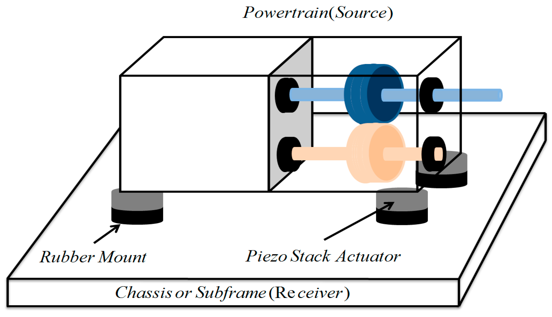
2. Modeling of Mounting System

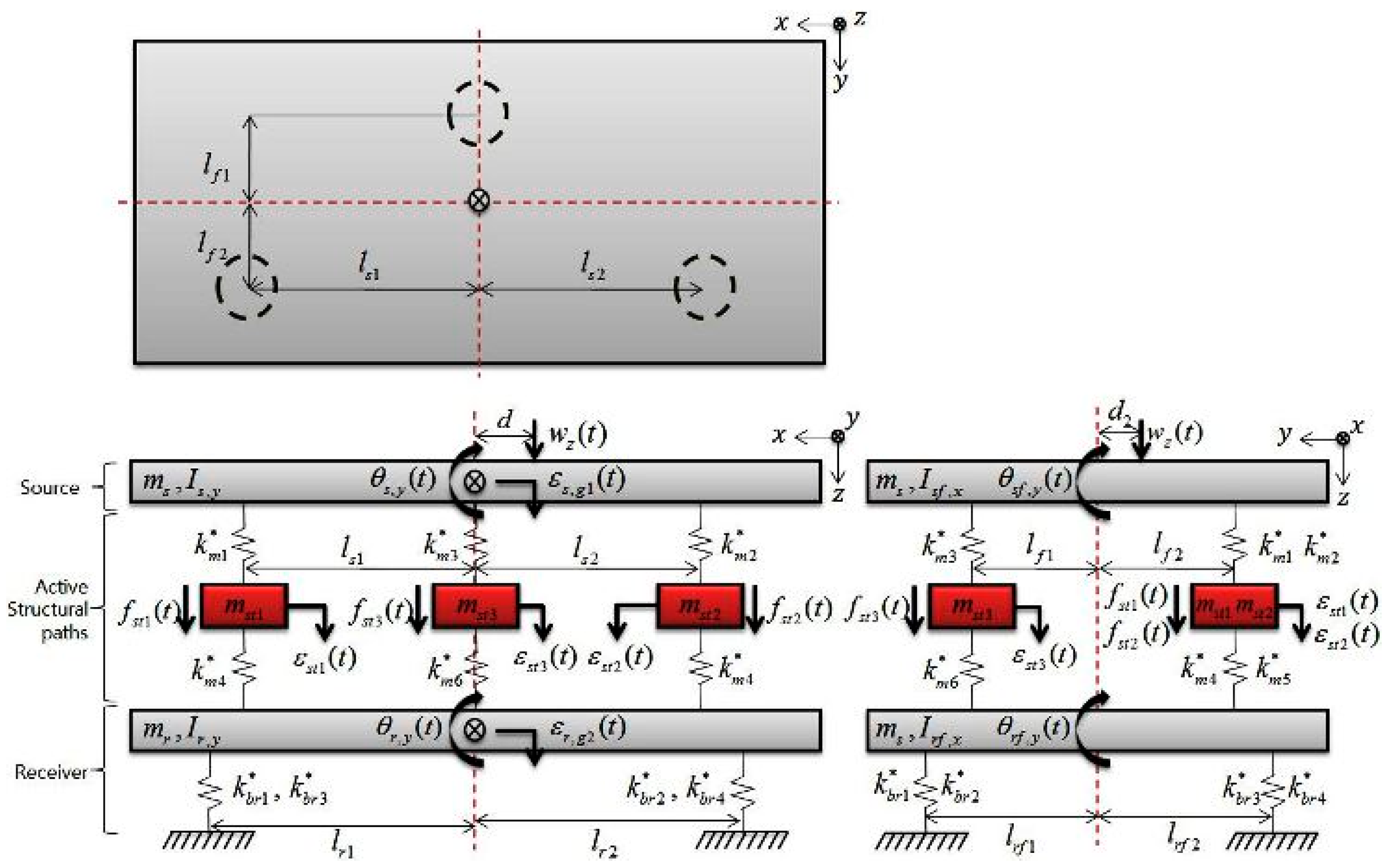
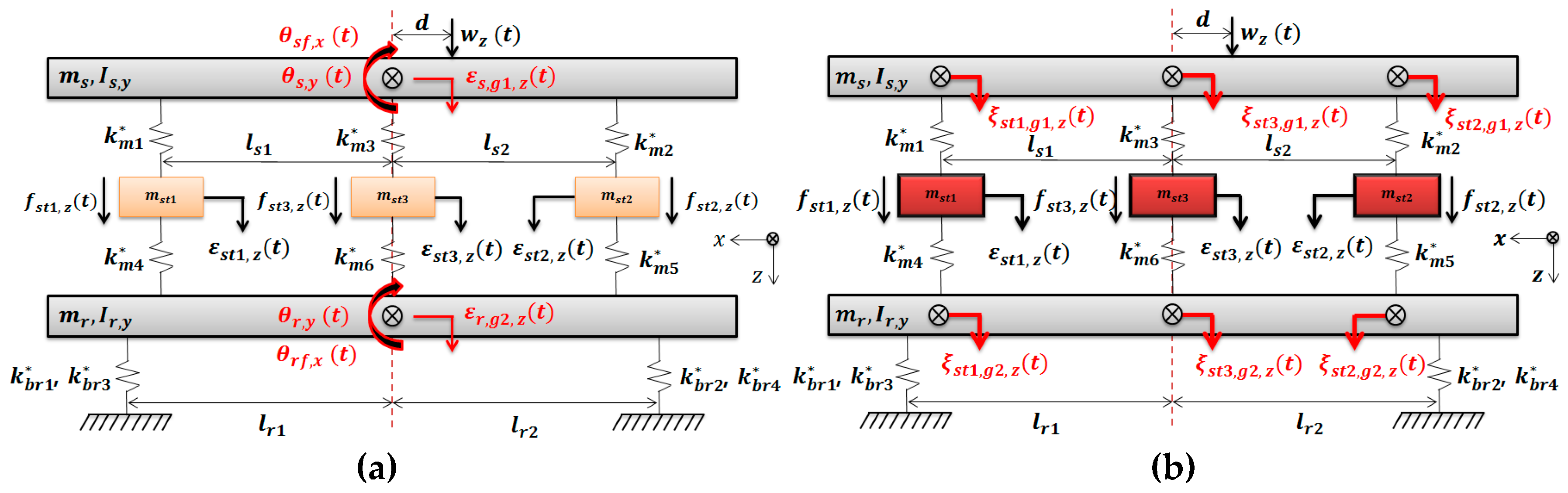
2.1. 9-DOF Modeling

The overall schematic of the 9-DOF mounting system is based on Figure 1 and modeled as shown in Figure 2.

The 3D model was created on the basis of the lumped parameter model and expressed using orthographic projection. The floor plan shows the location of the active structural paths; $m_s$, $m_r$, and $m_{st\hspace{0.17em}i}$ represent the source, receiver, and actuator mass, respectively, that were actually measured and used; $I_{s,y}$ and $I_{r,y}$ represent the inertia of the source and receiver, respectively, in the y-direction. $I_{sf,x}$ and $I_{rf,x}$ represent the inertia of the source and receiver, respectively, in the x-direction and were derived from calculations; $l_{si}$ and $l_{ri}$ represent the distance between each path on the front of the source and receiver, respectively; $l_{fi}$ and $l_{rfi}$ indicate the distance between each path on the sides of the source and receiver, respectively; $d$ and $d_2$ are the distances of the shaker relative to each direction; ${\theta }_{s,y}$, ${\theta }_{r,y}$, ${\theta }_{sf,x}$, and ${\theta }_{rf,x}$ represent the rotational displacement of the source and receiver relative to the front and side, respectively; $k_{mi}^{\ast }$ and $k_{bri}^{\ast }$ represent the complex stiffness for each path; ${\epsilon }_{s,g1,z}$ and ${\epsilon }_{r,g2,z}$ indicate the translational motion of the source and receiver, respectively; ${\epsilon }_{sti,z}$ and $f_{sti}$ represent the motion and force, respectively, of the ith actuator; $w_z$ represents the force of the shaker.

In this study, the translational motion assumed only the z-direction. The rotational displacement in the y-direction was assumed to be on the front. Only the x-direction was assumed to be on the sides. Moreover, the rotational displacement was assumed to be very small. The values of each parameter are summarized in

Table 1. Variable values and units for 9 degrees of freedom (DOF).

Variable	Values	Units	Variable	Values	Units
$m_s=m_r$	$1.081$	$\mathrm{kg}$	$k_{m5}^{\ast }$	$0.53(1+i0.256)$	$\mathrm{kN}\hspace{0.17em}{\mathrm{mm}}^{-1}$
$m_{st1}=m_{st3}$	$0.067$	$\mathrm{kg}$	$k_{m6}^{\ast }$	$0.61(1+i0.300)$	$\mathrm{kN}\hspace{0.17em}{\mathrm{mm}}^{-1}$
$m_{st2}$	$0.075$	$\mathrm{kg}$	$k_{brn\hspace{0.17em}(n=1,2)}^{\ast }$	$0.42(1+i0.300)$	$\mathrm{kN}\hspace{0.17em}{\mathrm{mm}}^{-1}$
$I_{s,y}=I_{r,y}$	$16.172$	$\mathrm{g}\hspace{0.17em}{\mathrm{m}}^2$	$l_{sn\hspace{0.17em}(n=1,2)}$	$100$	$\mathrm{mm}$
$I_{sf,x}=I_{rf,x}$	$5.940$	$\mathrm{g}\hspace{0.17em}{\mathrm{m}}^2$	$l_{rn\hspace{0.17em}(n=1,2)}$	$140$	$\mathrm{mm}$
$k_{m1}^{\ast }$	$5.46(1+i0.034)$	$\mathrm{kN}\hspace{0.17em}{\mathrm{mm}}^{-1}$	$l_{fn\hspace{0.17em}(n=1,2)}$	$80$	$\mathrm{mm}$
$k_{m2}^{\ast }$	$5.46(1+i0.034)$	$\mathrm{kN}\hspace{0.17em}{\mathrm{mm}}^{-1}$	$l_{rfn\hspace{0.17em}(n=1~4)}$	$100$	$\mathrm{mm}$
$k_{m3}^{\ast }$	$2.48(1+i0.036)$	$\mathrm{kN}\hspace{0.17em}{\mathrm{mm}}^{-1}$	$d$	$50$	$\mathrm{mm}$
$k_{m4}^{\ast }$	$0.61(1+i0.300)$	$\mathrm{kN}\hspace{0.17em}{\mathrm{mm}}^{-1}$	$d_2$	$10$	$\mathrm{mm}$

. Equations (1)–(9) express the equations of motion of the front and sides:

$$\begin{array}{ll}{m}_s{\ddot{\epsilon }}_{s,g1,z}& +(k_{m1}+k_{m3}+k_{m2}){\epsilon }_{s,g1,z}-k_{m1}{\epsilon }_{st1,z}-k_{m2}{\epsilon }_{st2,z}-k_{m3}{\epsilon }_{st3,z}\\ & +\left(k_{m2}{l}_{s2}-k_{m1}{\epsilon }_{s1}\right){\theta }_{s,y}+\left(k_{m1}{l}_{f1}+k_{m2}{l}_{f1}-k_{m3}{l}_{f2}\right){\theta }_{sf,x}=w_z(t)\end{array}$$

(1)

$$\begin{array}{ll}{m}_r{\ddot{\epsilon }}_{r,g1,z}& +(k_{m4}^{\ast }+k_{m5}^{\ast }+k_{m6}^{\ast }+k_{br1}^{\ast }+k_{br2}^{\ast }+k_{br3}^{\ast }+k_{br4}^{\ast }){\epsilon }_{r,g1,z}-k_{m4}^{\ast }{\epsilon }_{st1,z}-k_{m5}^{\ast }{\epsilon }_{st2,z}-k_{m6}^{\ast }{\epsilon }_{st3,z}\\ & +(k_{m5}^{\ast }{l}_{s1}-k_{m4}^{\ast }{l}_{s1}-k_{br1}^{\ast }{l}_{r1}+k_{br2}^{\ast }{l}_{r2}-k_{br3}^{\ast }{l}_{r3}+k_{br4}^{\ast }{l}_{r4}){\theta }_{r,y}\\ & +(k_{m4}^{\ast }{l}_{f1}+k_{m5}^{\ast }{l}_{f1}-k_{m6}^{\ast }{l}_{f2}-k_{br1}^{\ast }{l}_{rf1}-k_{br2}^{\ast }{l}_{rf2}+k_{br3}^{\ast }{l}_{rf3}+k_{br4}^{\ast }{l}_{rf4}){\theta }_{rf,x}=0\end{array}$$

(2)

$$\begin{array}{l}{m}_{st1}{\ddot{\epsilon }}_{st1,g1,z}+(k_{m1}^{\ast }+k_{m4}^{\ast }){\epsilon }_{st1,z}\\ \hspace{0.17em}-k_{m1}^{\ast }{\epsilon }_{s,g1,z}-k_{m4}^{\ast }{\epsilon }_{r,g1,z}+k_{m1}^{\ast }{l}_{s1}{\theta }_{s,y}+k_{m4}^{\ast }{l}_{s1}{\theta }_{r,y}-k_{m1}^{\ast }{l}_{f1}{\theta }_{sf,x}-k_{m4}^{\ast }{l}_{f1}{\theta }_{rf,x}=f_{st1,z}(t)\end{array}$$

(3)

$$\begin{array}{l}{m}_{st2}{\ddot{\epsilon }}_{st2,z}+(k_{m2}^{\ast }+k_{m5}^{\ast }){\epsilon }_{st2,z}\\ \hspace{0.17em}-k_{m2}^{\ast }{\epsilon }_{s,g1,z}-k_{m5}^{\ast }{\epsilon }_{r,g1,z}-k_{m2}^{\ast }{l}_{s2}{\theta }_{s,y}-k_{m5}^{\ast }{l}_{s2}{\theta }_{r,y}-k_{m2}^{\ast }{l}_{f1}{\theta }_{sf,x}-k_{m5}^{\ast }{l}_{f1}{\theta }_{rf,x}=f_{st2,z}(t)\end{array}$$

(4)

$$m_{st3}{\ddot{\epsilon }}_{st3,z}+(k_{m3}^{\ast }+k_{m6}^{\ast }){\epsilon }_{st3,z}-k_{m3}^{\ast }{\epsilon }_{s,g1,z}-k_{m6}^{\ast }{\epsilon }_{r,g1,z}-k_{m3}^{\ast }{l}_{f2}{\theta }_{sf,x}-k_{m6}^{\ast }{l}_{f2}{\theta }_{rf,x}=f_{st3,z}(t),$$

(5)

$$I_s{\ddot{\theta }}_{s,y}+(k_{m2}^{\ast }{l}_{s2}-k_{m1}^{\ast }{l}_{s1}){\epsilon }_{s,g1,z}+k_{m1}^{\ast }{l}_{s1}{\epsilon }_{st1,z}-k_{m2}^{\ast }{l}_{s2}{\epsilon }_{st2,z}+(k_{m2}^{\ast }{l}_{s2}^2+k_{m1}^{\ast }{l}_{s1}^2){\theta }_{s,y}=w_z(t)d$$

(6)

$$\begin{array}{l}{I}_r{\ddot{\theta }}_{r,y}+(k_{m5}^{\ast }{l}_{s2}-k_{m4}^{\ast }{l}_{s2}+k_{br2}^{\ast }{l}_{r2}-k_{br1}^{\ast }{l}_{r1}){\epsilon }_{r,g1,z}\\ \hspace{0.17em}+k_{m4}^{\ast }{l}_{s1}{\epsilon }_{st1,z}-k_{m5}^{\ast }{l}_{s2}{\epsilon }_{st2,z}+(k_{m4}^{\ast }{l}_{s1}^2+k_{m5}^{\ast }{l}_{s2}^2+k_{br1}^{\ast }{l}_{r1}^2+k_{br2}^{\ast }{l}_{r2}^2+k_{br3}^{\ast }{l}_{r3}^2+k_{br4}^{\ast }{l}_{r4}^2){\theta }_{r,y}=0\end{array}$$

(7)

$$\begin{array}{l}{I}_s{\ddot{\theta }}_{sf,x}+(k_{m1}^{\ast }{l}_{f1}+k_{m2}^{\ast }{l}_{f1}-k_{m3}^{\ast }{l}_{f2}){\epsilon }_{s,g1,z}\\ \hspace{0.17em}+k_{m3}^{\ast }{l}_{f2}{\epsilon }_{st3,z}-k_{m1}^{\ast }{l}_{f1}{\epsilon }_{st1,z}-k_{m2}^{\ast }{l}_{f1}{\epsilon }_{st2,z}+(k_{m1}^{\ast }{l}_{f1}^2+k_{m2}^{\ast }{l}_{f1}^2+k_{m3}^{\ast }{l}_{f2}^2){\theta }_{sf,x}=w_z(t)d_2\end{array}$$

(8)

$$\begin{array}{ll}{I}_r{\ddot{\theta }}_{rf,x}& +(k_{m4}^{\ast }{l}_{f1}+k_{m5}^{\ast }{l}_{f1}-k_{m6}^{\ast }{l}_{f2}-k_{br1}^{\ast }{l}_{rf1}-k_{br2}^{\ast }{l}_{rf3}+k_{br3}^{\ast }{l}_{rf2}+k_{br4}^{\ast }{l}_{rf4}){\epsilon }_{r,g1,z}\\ & +k_{m6}^{\ast }{l}_{f2}{\epsilon }_{st3,z}-k_{m4}^{\ast }{l}_{f1}{\epsilon }_{st1,z}-k_{m5}^{\ast }{l}_{f1}{\epsilon }_{st2,z}\\ & +(k_{m4}^{\ast }{l}_{f1}^2+k_{m5}^{\ast }{l}_{f1}^2+k_{m6}^{\ast }{l}_{f2}^2+k_{br1}^{\ast }{l}_{rf1}^2+k_{br2}^{\ast }{l}_{rf3}^2+k_{br3}^{\ast }{l}_{rf2}^2+k_{br4}^{\ast }{l}_{rf4}^2){\theta }_{rf,x}=0\end{array}$$

(9)

To express the equation of motion in a simple matrix form, the mass, stiffness, forces, and displacement vector are defined in Equations (10)–(14).

$$M=diag(\{m_s{m}_r{m}_{st1}{m}_{st2}{m}_{st3}{I}_{s,y}{I}_{r,y}{I}_{s,x}{I}_{r,x}\})$$

(10)

$$\begin{array}{l}{K}^{\ast }=[\begin{array}{ccccc}{k}_{m2}^{\ast }+k_{m3}^{\ast }+k_{m4}^{\ast }& 0& -k_{m1}^{\ast }& -k_{m2}^{\ast }& -k_{m3}^{\ast }\\ 0& k_{m4}^{\ast }+k_{m5}^{\ast }+k_{m6}^{\ast }+k_{br1}^{\ast }+k_{br2}^{\ast }& -k_{m4}^{\ast }& -k_{m5}^{\ast }& -k_{m6}^{\ast }\\ -k_{m1}^{\ast }& -k_{m4}^{\ast }& k_{m1}^{\ast }+k_{m4}^{\ast }& 0& 0\\ -k_{m2}^{\ast }& -k_{m5}^{\ast }& 0& k_{m2}^{\ast }+k_{m5}^{\ast }& 0\\ -k_{m3}^{\ast }& -k_{m6}^{\ast }& 0& 0& k_{m3}^{\ast }+k_{m6}^{\ast }\\ k_{m3}^{\ast }{l}_{s2}-k_{m1}^{\ast }{l}_{s1}& 0& k_{m1}^{\ast }{l}_{s1}& -k_{m2}^{\ast }{l}_{s2}& 0\\ 0& k_{m5}^{\ast }{l}_{s2}-k_{m4}^{\ast }{l}_{s1}-k_{br1}^{\ast }{l}_{r2}+k_{br2}^{\ast }{l}_{r2}& k_{m4}^{\ast }{l}_{s1}& -k_{m5}^{\ast }{l}_{s2}& 0\\ k_{m1}^{\ast }{l}_{f1}-k_{m2}^{\ast }{l}_{f1}-k_{m3}^{\ast }{l}_{f2}& 0& -k_{m1}^{\ast }{l}_{f1}& -k_{m2}^{\ast }{l}_{f1}& -k_{m3}^{\ast }{l}_{f2}\\ 0& k_{m4}^{\ast }{l}_{f1}-k_{m5}^{\ast }{l}_{f1}-k_{m6}^{\ast }{l}_{f2}& -k_{m4}^{\ast }{l}_{f1}& -k_{m5}^{\ast }{l}_{f1}& k_{m6}^{\ast }{l}_{f2}\end{array}\\ ---------------------------------------------------\\ \approx \begin{array}{cccc}{k}_{m3}^{\ast }{l}_{s2}-k_{m1}^{\ast }{l}_{s1}& 0& k_{m1}^{\ast }{l}_{f1}-k_{m2}^{\ast }{l}_{f1}-k_{m3}^{\ast }{l}_{f2}& 0\\ 0& k_{m5}^{\ast }{l}_{s2}-k_{m4}^{\ast }{l}_{s1}-k_{br1}^{\ast }{l}_{r2}+k_{br2}^{\ast }{l}_{r2}& 0& k_{m4}^{\ast }{l}_{f1}-k_{m5}^{\ast }{l}_{f1}-k_{m6}^{\ast }{l}_{f2}\\ k_{m1}^{\ast }{l}_{s1}& k_{m4}^{\ast }{l}_{s1}& -k_{m1}^{\ast }{l}_{f1}& -k_{m4}^{\ast }{l}_{f1}\\ -k_{m2}^{\ast }{l}_{s2}& -k_{m5}^{\ast }{l}_{s2}& -k_{m2}^{\ast }{l}_{f1}& -k_{m5}^{\ast }{l}_{f1}\\ 0& 0& -k_{m3}^{\ast }{l}_{f2}& k_{m6}^{\ast }{l}_{f2}\\ k_{m4}^{\ast }{l}_{s1}^2+k_{m2}^{\ast }{l}_{s2}^2& 0& 0& 0\\ 0& k_{br1}^{\ast }{l}_{r1}^2+k_{br2}^{\ast }{l}_{r2}^2+k_{m4}^{\ast }{l}_{s1}^2+k_{m5}^{\ast }{l}_{s2}^2& 0& 0\\ 0& 0& k_{m1}^{\ast }{l}_{f1}^2+k_{m2}^{\ast }{l}_{f1}^2+k_{m3}^{\ast }{l}_{f2}^2& 0\\ 0& 0& 0& k_{m4}^{\ast }{l}_{f1}^2+k_{m5}^{\ast }{l}_{f1}^2+k_{m6}^{\ast }{l}_{f2}^2\end{array}]\end{array}$$

(11)

$$q(t)=\left\{\begin{array}{c}{\epsilon }_{s,g1,z}(t)\\ {\epsilon }_{r,g1,z}(t)\\ {\epsilon }_{st1,z}(t)\\ {\epsilon }_{st2,z}(t)\\ {\epsilon }_{st3,z}(t)\\ {\theta }_{s,y}(t)\\ {\theta }_{r,y}(t)\\ {\theta }_{sf,x}(t)\\ {\theta }_{rf,x}(t)\end{array}\right\}$$

(12)

$$w(t)=\left\{\begin{array}{c}{w}_z(t)\\ 0\\ 0\\ 0\\ 0\\ w_z(t)d\\ 0\\ w_z(t)d_2\\ 0\end{array}\right\}$$

(13)

$$F(t)=\left\{\begin{array}{c}0\\ 0\\ f_{st1,z}(t)\\ f_{st2,z}(t)\\ f_{st3,z}(t)\\ 0\\ 0\\ 0\\ 0\end{array}\right\}$$

(14)

The focus of this study was on the vibration reduction effect by the active path. To investigate the vibration reduction performance of the part where each active path is located, a coordinate transformation was performed using the transfer matrix $\prod$ defined in Equation (15).

$$\prod =\left[\begin{array}{ccccccccc}\frac{l_{s1}}{l_{s1}+l_{s2}}& \frac{l_{s2}}{l_{s1}+l_{s2}}& \frac{l_{f2}}{l_{f1}+l_{f2}}& 0& 0& 0& 0& 0& 0\\ 0& 0& 0& 0& 0& 0& \frac{l_{s1}}{l_{s1}+l_{s2}}& \frac{l_{s2}}{l_{s1}+l_{s2}}& \frac{l_{f2}}{l_{f1}+l_{f2}}\\ 0& 0& 0& 1& 0& 0& 0& 0& 0\\ 0& 0& 0& 0& 1& 0& 0& 0& 0\\ 0& 0& 0& 0& 0& 1& 0& 0& 0\\ \frac{-1}{l_{s1}+l_{s2}}& \frac{1}{l_{s1}+l_{s2}}& 0& 0& 0& 0& 0& 0& 0\\ 0& 0& 0& 0& 0& 0& \frac{-1}{l_{s1}+l_{s2}}& \frac{1}{l_{s1}+l_{s2}}& 0\\ \frac{-1}{l_{s1}+l_{s2}}& \frac{-1}{l_{s1}+l_{s2}}& \frac{1}{l_{f1}+l_{f2}}& 0& 0& 0& 0& 0& 0\\ 0& 0& 0& 0& 0& 0& \frac{-1}{l_{s1}+l_{s2}}& \frac{-1}{l_{s1}+l_{s2}}& \frac{1}{l_{f1}+l_{f2}}\end{array}\right]$$

(15)

The transformed displacement is defined as $q=\prod q^{\prime }$, and the displacement matrix $q$ for each active path is redefined as shown in Equation (16). If the equation of motion is rewritten, it is expressed as Equation (17). The schematic representation of the transformed coordinates is shown in Figure 3.

$$q^{\prime }=\left\{\begin{array}{ccccccccc}{\xi }_{st1,g1,z}(t)& {\xi }_{st2g1,z}(t)& {\xi }_{st3,g1,z}(t)& {\epsilon }_{st1,z}(t)& {\epsilon }_{st2,z}(t)& {\epsilon }_{st3,z}(t)& {\xi }_{st1,g2,z}(t)& {\xi }_{st2,g2,z}(t)& {\xi }_{st3,g2,z}(t)\end{array}\right\}$$

(16)

$$M^{\prime }{\ddot{q}}^{\prime }+K^{\ast \prime }{q}^{\prime }=F(x)+W(t)$$

(17)

2.2. Calculation of Actuator Amplitude and Phase

To define the relationship between harmonic excitation and actuator response, each input is defined by Equations (18) and (19):

$$w_z(t)=W_z{e}^{i\omega t}$$

(18)

$$f_{st\hspace{0.17em}i,z}(t)=F_{st\hspace{0.17em}i,z}{e}^{i(\omega t+{\varphi }_{st\hspace{0.17em}i,z})}$$

(19)

where $W_Z$ is the amplitude of the shaker, and $F_{st\hspace{0.17em}i}$ and ${\varphi }_{st\hspace{0.17em}i}$ stand for the amplitude and phase of the actuator in the ith path, respectively. The displacement of the system according to the excitation force is defined for each active path and expressed by Equation (20):

$${\xi }_i^{\ast }(t)={\xi }_{sti,g1}^{\ast }(t)$$

(20)

${\xi }_{sti,g1}^{\ast }(t)$ is the displacement of the ith actuator with inertia $g_1$ and is affected by the excitation force of the shaker and each actuator. It can be defined by the Equations (21)–(23) as follows:

$${\xi }_1^{\ast }(t)=({\Xi }_{s1,1}^{\ast }+{\Xi }_{s1,st1}^{\ast }{e}^{i{\varphi }_{st1}}+{\Xi }_{s1,st2}^{\ast }{e}^{i{\varphi }_{st2}}+{\Xi }_{s1,st3}^{\ast }{e}^{i{\varphi }_{st3}})e^{i\omega t}$$

(21)

$${\xi }_2^{\ast }(t)=({\Xi }_{s2,1}^{\ast }+{\Xi }_{s2,st1}^{\ast }{e}^{i{\varphi }_{st1}}+{\Xi }_{s2,st2}^{\ast }{e}^{i{\varphi }_{st2}}+{\Xi }_{s2,st3}^{\ast }{e}^{i{\varphi }_{st3}})e^{i\omega t}$$

(22)

$${\xi }_3^{\ast }(t)=({\Xi }_{s3,1}^{\ast }+{\Xi }_{s3,st1}^{\ast }{e}^{i{\varphi }_{st1}}+{\Xi }_{s3,st2}^{\ast }{e}^{i{\varphi }_{st2}}+{\Xi }_{s3,st3}^{\ast }{e}^{i{\varphi }_{st3}})e^{i\omega t}$$

(23)

${\Xi }_{si,1}^{\ast }$ is the amplitude of the shaker, and ${\Xi }_{si,st1}^{\ast }$, ${\Xi }_{si,st2}^{\ast }$, and ${\Xi }_{si,st3}^{\ast }$ represent the amplitudes of the actuator for the ith active path. To calculate the amplitude and phase, a compliance matrix, represented by Equation (24), is used to define the amount of deformation caused by a unit load.

$$H^{\ast \prime }=\left[\begin{array}{ccccccccc}{H}_{11}^{\ast \prime }& H_{12}^{\ast \prime }& H_{13}^{\ast \prime }& H_{14}^{\ast \prime }& H_{15}^{\ast \prime }& H_{16}^{\ast \prime }& H_{17}^{\ast \prime }& H_{18}^{\ast \prime }& H_{19}^{\ast \prime }\\ H_{21}^{\ast \prime }& H_{22}^{\ast \prime }& H_{23}^{\ast \prime }& H_{24}^{\ast \prime }& H_{25}^{\ast \prime }& H_{26}^{\ast \prime }& H_{27}^{\ast \prime }& H_{28}^{\ast \prime }& H_{29}^{\ast \prime }\\ H_{31}^{\ast \prime }& H_{32}^{\ast \prime }& H_{33}^{\ast \prime }& H_{34}^{\ast \prime }& H_{35}^{\ast \prime }& H_{36}^{\ast \prime }& H_{37}^{\ast \prime }& H_{38}^{\ast \prime }& H_{39}^{\ast \prime }\\ H_{41}^{\ast \prime }& H_{42}^{\ast \prime }& H_{43}^{\ast \prime }& H_{44}^{\ast \prime }& H_{45}^{\ast \prime }& H_{46}^{\ast \prime }& H_{47}^{\ast \prime }& H_{48}^{\ast \prime }& H_{49}^{\ast \prime }\\ H_{51}^{\ast \prime }& H_{52}^{\ast \prime }& H_{53}^{\ast \prime }& H_{54}^{\ast \prime }& H_{55}^{\ast \prime }& H_{56}^{\ast \prime }& H_{57}^{\ast \prime }& H_{58}^{\ast \prime }& H_{59}^{\ast \prime }\\ H_{61}^{\ast \prime }& H_{62}^{\ast \prime }& H_{63}^{\ast \prime }& H_{64}^{\ast \prime }& H_{65}^{\ast \prime }& H_{66}^{\ast \prime }& H_{67}^{\ast \prime }& H_{68}^{\ast \prime }& H_{69}^{\ast \prime }\\ H_{71}^{\ast \prime }& H_{72}^{\ast \prime }& H_{73}^{\ast \prime }& H_{74}^{\ast \prime }& H_{75}^{\ast \prime }& H_{76}^{\ast \prime }& H_{77}^{\ast \prime }& H_{78}^{\ast \prime }& H_{79}^{\ast \prime }\\ H_{81}^{\ast \prime }& H_{82}^{\ast \prime }& H_{83}^{\ast \prime }& H_{84}^{\ast \prime }& H_{85}^{\ast \prime }& H_{86}^{\ast \prime }& H_{87}^{\ast \prime }& H_{88}^{\ast \prime }& H_{89}^{\ast \prime }\\ H_{91}^{\ast \prime }& H_{92}^{\ast \prime }& H_{93}^{\ast \prime }& H_{94}^{\ast \prime }& H_{95}^{\ast \prime }& H_{96}^{\ast \prime }& H_{97}^{\ast \prime }& H_{98}^{\ast \prime }& H_{99}^{\ast \prime }\end{array}\right]$$

(24)

The amplitude displacement vector for each active path is defined in Equation (25):

$$Q^{\ast \prime }=\left\{{\Xi }_{st1,g1}^{\ast }{\Xi }_{st2,g1}^{\ast }{\Xi }_{st3,g1}^{\ast }{\wp }_{st1}^{\ast }{\wp }_{st2}^{\ast }{\wp }_{st3}^{\ast }{\Xi }_{st1,g2}^{\ast }{\Xi }_{st2,g2}^{\ast }{\Xi }_{st3,g2}^{\ast }\right\}$$

(25)

The amplitude is calculated by Equation (26):

$$Q^{\ast \prime }{e}^{i\omega t}=H^{\ast \prime }\left\{F^{\ast }+W^{\ast }\right\}{e}^{i\omega t}$$

(26)

The amplitudes generated from the active paths are defined by Equations (27)–(29).

$$\begin{array}{l}{\Xi }_{s1,1}^{\ast }=(H_{11}^{\ast \prime }+H_{16}^{\ast \prime }d+H_{18}^{\ast \prime }d)W_z\\ {\Xi }_{s1,st1}^{\ast }=H_{13}^{\ast \prime }{F}_{st1},{\Xi }_{s1,st2}^{\ast }=H_{14}^{\ast \prime }{F}_{st2},{\Xi }_{s1,st3}^{\ast }=H_{15}^{\ast \prime }{F}_{st3}\end{array}$$

(27)

$$\begin{array}{l}{\Xi }_{s2,1}^{\ast }=(H_{21}^{\ast \prime }+H_{26}^{\ast \prime }d+H_{28}^{\ast \prime }d)W_z\\ {\Xi }_{s2,st1}^{\ast }=H_{23}^{\ast \prime }{F}_{st1},{\Xi }_{s2,st2}^{\ast }=H_{24}^{\ast \prime }{F}_{st2},{\Xi }_{s2,st3}^{\ast }=H_{25}^{\ast \prime }{F}_{st3}\end{array}$$

(28)

$$\begin{array}{l}{\Xi }_{s3,1}^{\ast }=(H_{31}^{\ast \prime }+H_{36}^{\ast \prime }d+H_{38}^{\ast \prime }d)W_z\\ {\Xi }_{s3,st1}^{\ast }=H_{33}^{\ast \prime }{F}_{st1},{\Xi }_{s3,st2}^{\ast }=H_{34}^{\ast \prime }{F}_{st2},{\Xi }_{s3,st3}^{\ast }=H_{35}^{\ast \prime }{F}_{st3}\end{array}$$

(29)

The phases, defined by Equations (30)–(32), are defined on the basis of amplitude:

$$\begin{array}{l}{\beta }_{s1,1}=\angle (H_{11}^{\prime }+H_{16}^{\prime }d+H_{18}^{\prime }d)\\ {\beta }_{s1,st1}=\angle H_{13}^{\prime },{\beta }_{s1,st2}=\angle H_{14}^{\prime },{\beta }_{s1,st3}=\angle H_{15}^{\prime }\end{array}$$

(30)

$$\begin{array}{l}{\beta }_{s2,1}=\angle (H_{21}^{\prime }+H_{26}^{\prime }d+H_{28}^{\prime }d)\\ {\beta }_{s2,st1}=\angle H_{23}^{\prime },{\beta }_{s2,st2}=\angle H_{24}^{\prime },{\beta }_{s2,st3}=\angle H_{25}^{\prime }\end{array}$$

(31)

$$\begin{array}{l}{\beta }_{s3,1}=\angle (H_{31}^{\prime }+H_{36}^{\prime }d+H_{38}^{\prime }d)\\ {\beta }_{s3,st1}=\angle H_{33}^{\prime },{\beta }_{s3,st2}=\angle H_{34}^{\prime },{\beta }_{s3,st3}=\angle H_{35}^{\prime }\end{array}$$

(32)

where $\angle$ stands for the phase operator, and ${\beta }_{sn,1}$ represents the phase of the amplitude generated by the shaker in the nth active path; ${\beta }_{sn,stm}$ represents the phase of the amplitude generated by the mth actuator in the nth active path. Using Equations (27)–(32), the magnitude and phase terms are defined by Equations (33)–(35):

$${\xi }_1^{\ast }(t)=\left(\left|{\Xi }_{s1,1}^{\ast }\right|e^{i{\beta }_{s1,1}}+\left|{\Xi }_{s1,st1}^{\ast }\right|e^{i\left({\beta }_{s1,st1}+{\varphi }_{st1}\right)}+\left|{\Xi }_{s1,st2}^{\ast }\right|e^{i\left({\beta }_{s1,st2}+{\varphi }_{st2}\right)}+\left|{\Xi }_{s1,st3}^{\ast }\right|e^{i\left({\beta }_{s1,st3}+{\varphi }_{st3}\right)}\right)e^{i\omega t}$$

(33)

$${\xi }_2^{\ast }(t)=\left(\left|{\Xi }_{s2,1}^{\ast }\right|e^{i{\beta }_{s2,1}}+\left|{\Xi }_{s2,st1}^{\ast }\right|e^{i\left({\beta }_{s2,st1}+{\varphi }_{st1}\right)}+\left|{\Xi }_{s2,st2}^{\ast }\right|e^{i\left({\beta }_{s2,st2}+{\varphi }_{st2}\right)}+\left|{\Xi }_{s2,st3}^{\ast }\right|e^{i\left({\beta }_{s2,st3}+{\varphi }_{st3}\right)}\right)e^{i\omega t}$$

(34)

$${\xi }_3^{\ast }(t)=\left(\left|{\Xi }_{s3,1}^{\ast }\right|e^{i{\beta }_{s3,1}}+\left|{\Xi }_{s3,st1}^{\ast }\right|e^{i\left({\beta }_{s3,st1}+{\varphi }_{st1}\right)}+\left|{\Xi }_{s3,st2}^{\ast }\right|e^{i\left({\beta }_{s3,st2}+{\varphi }_{st2}\right)}+\left|{\Xi }_{s3,st3}^{\ast }\right|e^{i\left({\beta }_{s3,st3}+{\varphi }_{st3}\right)}\right)e^{i\omega t}$$

(35)

These equations have seven-phase terms in one equation. Each phase has four phases that are generated by the shaker and actuator and three phases that occur only in the actuator. Because of the presence of various phases, it is difficult to control the motion. Therefore, we can assume that the phases generated by the shaker match each other. By this definition, it is possible to create a phase difference motion in each active path. The expression of phase for active path 1 can be written as ${\beta }_{s1,1}={\beta }_{s1,st1}+{\varphi }_{st1}$. Similarly, the phases for active paths 2 and 3 are ${\beta }_{s1,1}={\beta }_{s1,st2}+{\varphi }_{st2}$ and ${\beta }_{s1,1}={\beta }_{s1,st3}+{\varphi }_{st3}$, respectively. The phases generated by the shaker are represented by Equations (36)–(38):

$${\varphi }_{st1}={\beta }_{s1,1}-{\beta }_{s1,st1}$$

(36)

$${\varphi }_{st2}={\beta }_{s1,1}-{\beta }_{s1,st2}$$

(37)

$${\varphi }_{st2}={\beta }_{s1,1}-{\beta }_{s1,st2}$$

(38)

From Equations (36)–(38), the phase of the actuator in each active path caused an out-of-phase motion owing to the difference between the phase generated by the shaker and that of each path generated by the actuator. In the case of active paths 2 and 3, the phase of each actuator is defined as ${\varphi }_{st1}={\beta }_{s2,1}-{\beta }_{s2,st1}$, ${\varphi }_{st2}={\beta }_{s2,1}-{\beta }_{s2,st2}$, and ${\varphi }_{st3}={\beta }_{s2,1}-{\beta }_{s2,st3}$; and ${\varphi }_{st1}={\beta }_{s3,1}-{\beta }_{s3,st1}$, ${\varphi }_{st2}={\beta }_{s3,1}-{\beta }_{s3,st2}$, and ${\varphi }_{st3}={\beta }_{s3,1}-{\beta }_{s3,st3}$, respectively. Equations (39)–(41) are obtained by substituting the equation of the actuator phase into Equations (33)–(35) and summarizing them to determine the phase of the shaker:

$${\xi }_1^{\ast }(t)=\left(\left|{\Xi }_{s1,1}^{\ast }\right|+\left|{\Xi }_{s1,st1}^{\ast }\right|+\left|{\Xi }_{s1,st2}^{\ast }\right|+\left|{\Xi }_{s1,st3}^{\ast }\right|\right)e^{i\left(\omega t+{\beta }_{s1,1}\right)}$$

(39)

$${\xi }_2^{\ast }(t)=\left(\left|{\Xi }_{s2,1}^{\ast }\right|+\left|{\Xi }_{s2,st1}^{\ast }\right|+\left|{\Xi }_{s2,st2}^{\ast }\right|+\left|{\Xi }_{s2,st3}^{\ast }\right|\right)e^{i\left(\omega t+{\beta }_{s2,1}\right)}$$

(40)

$${\xi }_3^{\ast }(t)=\left(\left|{\Xi }_{s3,1}^{\ast }\right|+\left|{\Xi }_{s3,st1}^{\ast }\right|+\left|{\Xi }_{s3,st2}^{\ast }\right|+\left|{\Xi }_{s3,st3}^{\ast }\right|\right)e^{i\left(\omega t+{\beta }_{s3,1}\right)}$$

(41)

To reduce the motion to zero, the amplitudes $F_{st1,z}$, $F_{st2,z}$, and $F_{st3,z}$ of each actuator are calculated assuming that their magnitude is zero. Hence, we define Equations (42)–(44):

$$\left|{\Xi }_{s1,1}^{\ast }\right|+\left|{\Xi }_{s1,st1}^{\ast }\right|+\left|{\Xi }_{s1,st2}^{\ast }\right|+\left|{\Xi }_{s1,st3}^{\ast }\right|=0$$

(42)

$$\left|{\Xi }_{s2,1}^{\ast }\right|+\left|{\Xi }_{s2,st1}^{\ast }\right|+\left|{\Xi }_{s2,st2}^{\ast }\right|+\left|{\Xi }_{s2,st3}^{\ast }\right|=0$$

(43)

$$\left|{\Xi }_{s3,1}^{\ast }\right|+\left|{\Xi }_{s3,st1}^{\ast }\right|+\left|{\Xi }_{s3,st2}^{\ast }\right|+\left|{\Xi }_{s3,st3}^{\ast }\right|=0$$

(44)

To determine $F_{st1}$,$F_{st2}$, and $F_{st3}$, Equation (45) is given:

$$\left[\begin{array}{ccc}\left|H_{13}^{\ast }\right|& \left|H_{14}^{\ast }\right|& \left|H_{15}^{\ast }\right|\\ \left|H_{23}^{\ast }\right|& \left|H_{24}^{\ast }\right|& \left|H_{25}^{\ast }\right|\\ \left|H_{33}^{\ast }\right|& \left|H_{34}^{\ast }\right|& \left|H_{35}^{\ast }\right|\end{array}\right]\left\{\begin{array}{c}{F}_{st1}\\ F_{st2}\\ F_{st3}\end{array}\right\}=-W_z\left[\begin{array}{c}\left|H_{11}^{\ast }+d{H}_{16}^{\ast }+d{H}_{18}^{\ast }\right|\\ \left|H_{21}^{\ast }+d{H}_{26}^{\ast }+d{H}_{28}^{\ast }\right|\\ \left|H_{31}^{\ast }+d{H}_{36}^{\ast }+d{H}_{38}^{\ast }\right|\end{array}\right]$$

(45)

Equation (46) is used to calculate the amplitude of each actuator:

$$\begin{array}{ll}\left\{\begin{array}{c}{F}_{st1}\\ F_{st2}\\ F_{st3}\end{array}\right\}=& \frac{W_z}{\left|H_{13}^{\ast }\right|\left|H_{24}^{\ast }\right|\left|H_{35}^{\ast }\right|-\left|H_{13}^{\ast }\right|\left|H_{25}^{\ast }\right|\left|H_{34}^{\ast }\right|-\left|H_{14}^{\ast }\right|\left|H_{23}^{\ast }\right|\left|H_{35}^{\ast }\right|+\left|H_{14}^{\ast }\right|\left|H_{25}^{\ast }\right|\left|H_{33}^{\ast }\right|+\left|H_{15}^{\ast }\right|\left|H_{23}^{\ast }\right|\left|H_{34}^{\ast }\right|-\left|H_{15}^{\ast }\right|\left|H_{24}^{\ast }\right|\left|H_{33}^{\ast }\right|}\times \\ & \left[\begin{array}{l}\begin{array}{l}\left(\left|H_{14}^{\ast }\right|\left|H_{34}^{\ast }\right|-\left|H_{15}^{\ast }\right|\left|H_{34}^{\ast }\right|\right)\left(\left|H_{21}^{\ast }+d{H}_{26}^{\ast }+d{H}_{28}^{\ast }\right|\right)-\left(\left|H_{24}^{\ast }\right|\left|H_{35}^{\ast }\right|-\left|H_{25}^{\ast }\right|\left|H_{34}^{\ast }\right|\right)\left(\left|H_{11}^{\ast }+d{H}_{16}^{\ast }+d{H}_{18}^{\ast }\right|\right)\\ -\left(\left|H_{14}^{\ast }\right|\left|H_{25}^{\ast }\right|-\left|H_{15}^{\ast }\right|\left|H_{24}^{\ast }\right|\right)\left(\left|H_{31}^{\ast }+d{H}_{36}^{\ast }+d{H}_{38}^{\ast }\right|\right)\end{array}\\ \begin{array}{l}\left(\left|H_{23}^{\ast }\right|\left|H_{35}^{\ast }\right|-\left|H_{25}^{\ast }\right|\left|H_{33}^{\ast }\right|\right)\left(\left|H_{11}^{\ast }+d{H}_{16}^{\ast }+d{H}_{18}^{\ast }\right|\right)-\left(\left|H_{14}^{\ast }\right|\left|H_{25}^{\ast }\right|-\left|H_{15}^{\ast }\right|\left|H_{23}^{\ast }\right|\right)\left(\left|H_{31}^{\ast }+d{H}_{36}^{\ast }+d{H}_{38}^{\ast }\right|\right)\\ -\left(\left|H_{13}^{\ast }\right|\left|H_{35}^{\ast }\right|-\left|H_{15}^{\ast }\right|\left|H_{33}^{\ast }\right|\right)\left(\left|H_{21}^{\ast }+d{H}_{26}^{\ast }+d{H}_{28}^{\ast }\right|\right)\end{array}\\ \begin{array}{l}\left(\left|H_{13}^{\ast }\right|\left|H_{34}^{\ast }\right|-\left|H_{14}^{\ast }\right|\left|H_{33}^{\ast }\right|\right)\left(\left|H_{21}^{\ast }+d{H}_{26}^{\ast }+d{H}_{28}^{\ast }\right|\right)-\left(\left|H_{23}^{\ast }\right|\left|H_{34}^{\ast }\right|-\left|H_{24}^{\ast }\right|\left|H_{33}^{\ast }\right|\right)\left(\left|H_{11}^{\ast }+d{H}_{16}^{\ast }+d{H}_{18}^{\ast }\right|\right)\\ -\left(\left|H_{13}^{\ast }\right|\left|H_{24}^{\ast }\right|-\left|H_{14}^{\ast }\right|\left|H_{23}^{\ast }\right|\right)\left(\left|H_{31}^{\ast }+d{H}_{36}^{\ast }+d{H}_{38}^{\ast }\right|\right)\end{array}\end{array}\right]\end{array}$$

(46)

3. Validation Using the Numerical Simulation

3.1. Simulation Overview

Simulations were conducted to determine the validity of the mathematical model. The input and sampling frequencies were set to $u(t)=10\sin (800\pi t)$ and 15 kHz, respectively. The equations of motion were expressed using the state space equations and are represented by Equations (47) and (48):

$${\dot{x}}^{\prime }(t)=A{x}^{\prime }(t)+Bu(t)$$

(47)

$$y^{\prime }(t)=C{x}^{\prime }(t)+Du(t)$$

(48)

where $A$ is a matrix representing the state of the system, $B$ is an input matrix, and $C$ is an output matrix. Each matrix is expressed by Equations (49)–(52). In addition, the output $y(t)$ for the system has six outputs owing to three source and three receiver parts for the active path and is expressed by Equation (53):

$$A=\left[\begin{array}{cc}{O}_{n\times n}& I_{n\times n}\\ -\frac{K^{\prime }}{M^{\prime }}& -\frac{C^{\prime }}{M^{\prime }}\end{array}\right]$$

(49)

$$B=\left[\begin{array}{c}{O}_{n\times n}\\ \frac{1}{M^{\prime }}\end{array}\right]$$

(50)

$$C=\left[\begin{array}{ccc}{I}_{3\times 3}& O_{3\times 3}& O_{3\times 3}\\ O_{3\times 3}& O_{3\times 3}& I_{3\times 3}\end{array}{O}_{9\times 9}\right]$$

(51)

$$D=\left[O_{6\times 9}\right]$$

(52)

$$y(t)={\left\{a_{p1,g1}{a}_{p2,g1}{a}_{p3,g1}{a}_{p1,g2}{a}_{p2,g2}{a}_{p3,g2}\right\}}^T$$

(53)

where $a_{pn,gm}$ represents the acceleration in the nth path in mass with the inertia of m.

Although the state of the system that can be measured is limited, a total state value for the system is required to construct the feedback control system. Hence, a state observer wa designed as shown in Figure 4.

Using the real system matrices, A, B, and C, the G, H, and C matrices wre constructed for the estimates. Because the state space equations are defined in continuous time, they were transformed into discrete time matrices through bilinear transformation. The observer gain L was selected appropriately, and the agreement between the estimated and actual output was confirmed, as shown in Figure 5. Therefore, the validity of the model was verified, and it was applied to the feedback control system.

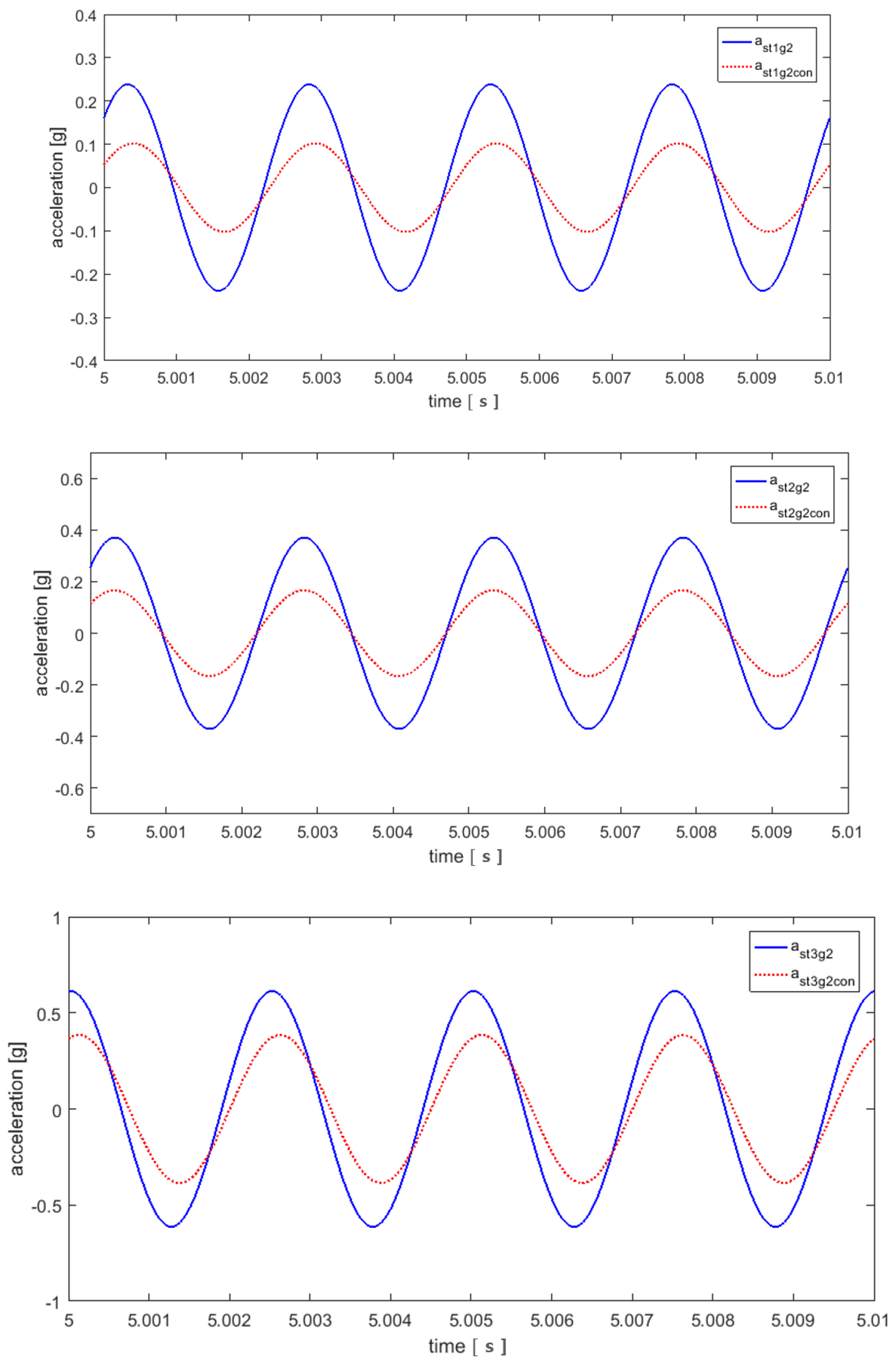
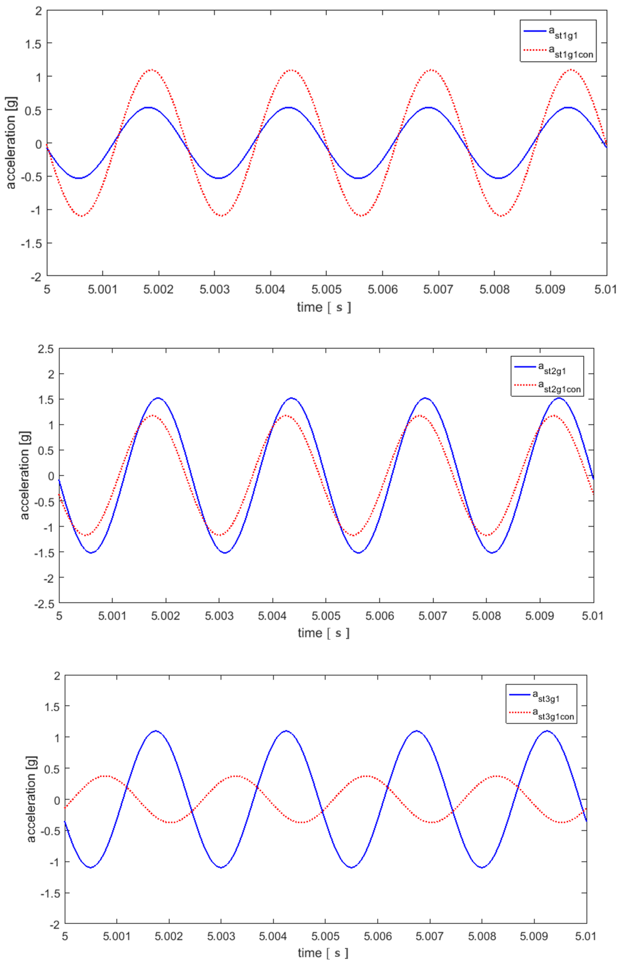
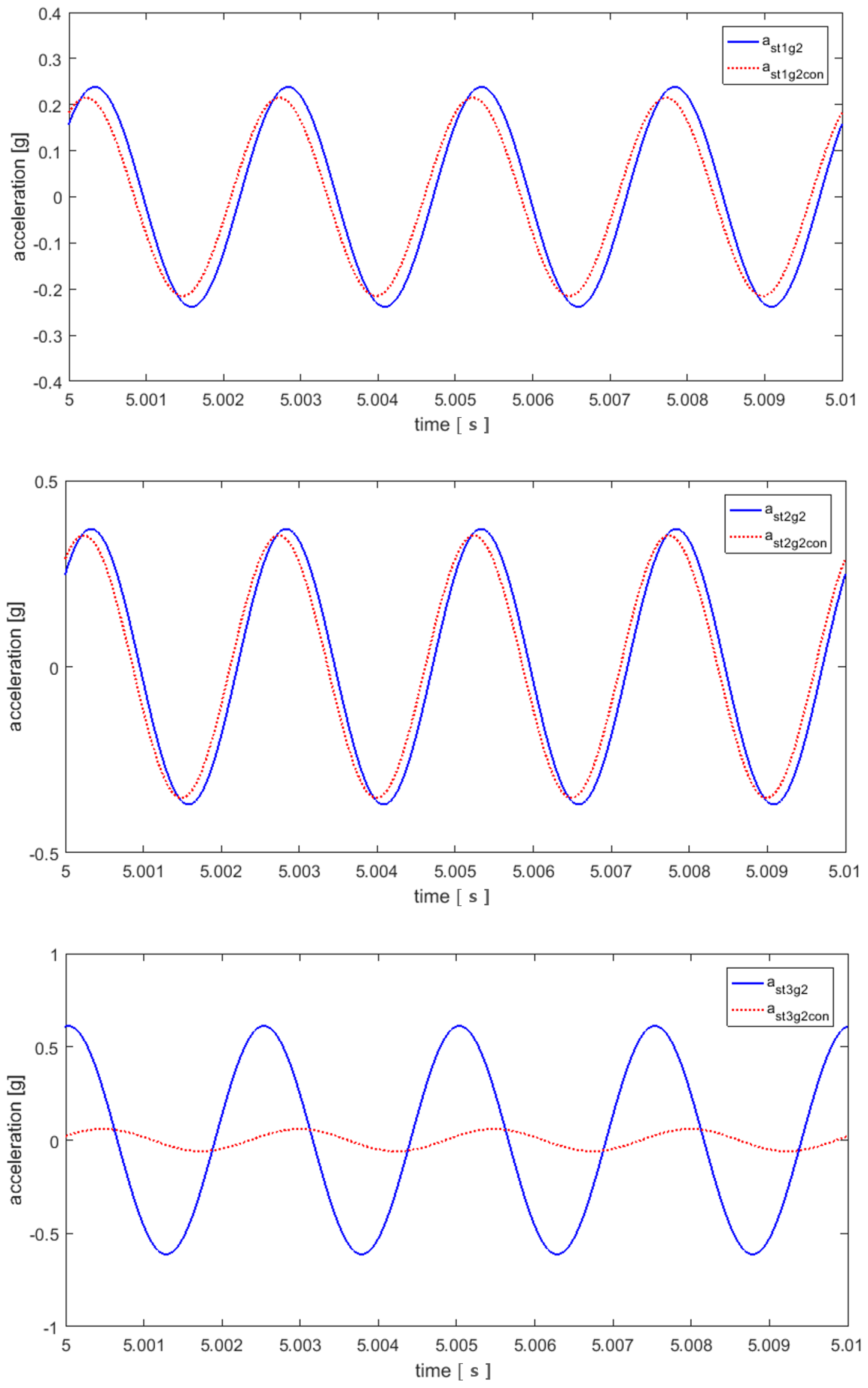
3.2. Control Using the Calculated Amplitude and Phase

A simulation was performed to determine whether the vibration transmitted to the source and receiver was reduced using the amplitude and phase values of the calculated actuator. The equations for the actuator input are defined by Equations (54)–(56):

$$f_{st1}(t)=F_{st1}\sin (\omega t+{\varphi }_{st1})$$

(54)

$$f_{st2}(t)=F_{st2}\sin (\omega t+{\varphi }_{st2})$$

(55)

$$f_{st3}(t)=F_{st3}\sin (\omega t+{\varphi }_{st3})$$

(56)

The simulation was performed with active path 3 as a target, and it was confirmed whether the vibration transmitted to the source and receiver were reduced when the actuators in all active paths were turned on. Figure 6 and Figure 7 show the results of the vibration of the source and receiver, respectively.

Table 2. Vibration reduction when the actuator was turned on.

Source	$a_{st1,g1}$	$a_{st2,g1}$	$a_{st3,g1}$
Original	$0.533$	$1.514$	$1.095$
All actuators turned on	$2.934\left(450.47\%\uparrow \right)$	$2.896\left(91.28\%\uparrow \right)$	$0.019\left(98.19\%\downarrow \right)$
Receiver	$a_{st1,g2}$	$a_{st2,g2}$	$a_{st3,g2}$
Original	$0.2382$	$0.37$	$0.6122$
All actuators turned on	$0.1021\left(57.13\%\downarrow \right)$	$0.165\left(55.18\%\downarrow \right)$	$0.384\left(37.21\%\downarrow \right)$

shows the values of the source and receiver outputs.

The results in Table 2 show that the vibration of $a_{st3,g1}$ was sharply reduced by about 98.19% because the active path 3 was used to calculate the actuator value for vibration isolation purposes. For $a_{st1,g1}$ and $a_{st2,g1}$, which were untargeted, the source vibration values were greatly increased by about 450.47% and 91.28%, respectively. However, the receiver results show that the vibration of $a_{st1,g2}$ was reduced by about 57% when compared to the uncontrolled results. The vibrations of $a_{st2,g2}$ and $a_{st3,g2}$ were decreased by about 55 and 37%, respectively.

3.3. Control Using the NLMS Algorithm

To isolate the source vibration of the target path in the previous section, the amplitude and phase of the actuator were calculated. However, it is evident that the vibration was greatly increased for the untargeted path. In addition, the calculation method cannot be applied to a signal with a real multi-frequency. Therefore, both the source and the receiver cannot control vibrations satisfactorily. Therefore, to compare with the computational isolation method, the simulation was carried out for the source and receiver vibration isolation using the NLMS algorithm. The simulation was based on the schematic representation shown in Figure 8 and was used as an input to the actuator using the signal from the source.

The inputs of the simulations were provided under the same conditions for comparison, and the signals entering the actuator were applied by appropriate adjustments to the signals from the NLMS algorithm. The simulation results of the source and receiver are shown in Figure 9 and Figure 10, respectively.

Table 3. Result of vibration reduction when the actuator was turned on using the NLMS signal.

Source	$a_{st1,g1}$	$a_{st2,g1}$	$a_{st3,g1}$
Original	$0.533$	$1.514$	$1.095$
Control using the NLMS	$1.096\left(105.62\%\uparrow \right)$	$1.171\left(22.66\%\downarrow \right)$	$0.374\left(65.84\%\downarrow \right)$
Receiver	$a_{st1,g2}$	$a_{st2,g2}$	$a_{st3,g2}$
Original	$0.2382$	$0.37$	$0.6122$
Control using the NLMS	$0.214\left(10.08\%\downarrow \right)$	$0.352\left(4.86\%\downarrow \right)$	$0.059\left(90.29\%\downarrow \right)$

presents the values for each output.

The result of the source part of Table 3 shows that the vibration of $a_{st1,g1}$ increased by about 105.62% compared to the previous value, but those of $a_{st2,g1}$ and $a_{st3,g1}$ decreased by 22.66 and 65.84%, respectively. In addition, the results for the receiver show that the vibrations of $a_{st1,g2}$, $a_{st2,g2}$, and $a_{st3,g2}$ decreased by 10.08, 4.86, and 90.29%, respectively. The reduction effect on the receiver was generally good for the calculation. However, when the results of the calculation in the source part wee compared with the those of the control using NLMS, the vibrations of $a_{st1,g1}$ and $a_{st2,g1}$ tended to greatly increase in the calculation method, but the result of using the NLMS algorithm tended to decrease the vibration in $a_{st2,g1}$. Moreover, the result of the calculation of vibration for $a_{st1,g1}$ showed a tendency to increase by 450.47%, which is about 5.5 times, whereas for the result using the NLMS algorithm, the vibration tended to increase by 105.62%, i.e., it doubled. Therefore, it can be seen that the use of the NLMS algorithm in the calculation method is more efficient for the whole system than the use of the actuator input.

4. Conclusions

This study was conducted to reduce vibration by coupling a piezo actuator and rubber mount between the plates of vehicle engines. The main contributions of this study are as follows: (1) Based on the source–path–receiver structure, three-dimensional motion equations for three active-path structures were established. Considering the effects on lateral rotational displacement, this enables a more realistic simulation compared to the modeling established in previous studies. (2) The NLMS algorithm was applied to the active control and compared to the calculation method of the actuator input. Through this result, it was shown that applying the NLMS algorithm is effective for overall vibration reduction.

The plate structure with active paths was modeled on the basis of the lumped parameter model and expressed using the equation of motion. When excited by a single frequency, the vibration-reduced effects were evaluated by comparing the results obtained by using the actuator input with those obtained by applying the NLMS algorithm. The computing method using the actuator input showed that the vibration of the receiver was largely reduced. However, the vibration of the non-targeted source was greatly increased. Moreover, this method is troublesome because it requires to newly define the modeling according to the structure change and cannot be applied when a multi-frequency input is applied. To solve this inconvenience, the NLMS algorithm was applied. When the NLMS algorithm was used, the vibration for the active path 1 in the source tended to increase, but those of the other active paths tended to reduce overall in the source and receiver. In particular, it was seen that the vibration of the active path 3 was largely isolated. Hence, future works should be conducted to study the relationship between each active path to control vibration more efficiently. In addition, an experimental verification of the results of this study should be carried out. Finally, our results show that vibrations are reduced for single-frequency inputs; hence, simulation and experiments for multi-frequency signals should be performed in the future.

References

1. Minak, G.; Fragassa, C.; De Camargo, F.V. A Brief Review on Determinant Aspects in Energy Efficient Solar Car Design and Manufacturing. In Proceedings of the International Conference on Sustainable Design and Manufacturing, Bologna, Italy, 26–28 April 2017; Volume 68, pp. 847–856. [Google Scholar]
2. Hosseini, A.M.; Arzanpour, S.; Golnaraghi, F.; Parameswaran, A.M. Solenoid actuator design and modeling with application in engine vibration isolators. J. Vib. Control 2012, 19, 1015–1023. [Google Scholar] [CrossRef]
3. Tang, X.; Yang, W.; Hu, X.; Zhang, D. A novel simplified model for torsional vibration analysis of a series-parallel hybrid electric vehicle. Mech. Syst. Signal Process. 2017, 85, 329–338. [Google Scholar] [CrossRef]
4. Kraus, R.; Herold, S.; Millitzer, J.; Jungblut, T. Development of Active Engine Mounts Based on Piezo Actuators. ATZ Worldw. 2014, 116, 46–51. [Google Scholar] [CrossRef]
5. Harun, M.H.; Azhari, M.A.; Yunos, M.R.M.; Yamin, A.K.M. Characterization of a Magnetorheological Fluid Damper Applied to Semi-Active Engine Mounting System. In Proceedings of the 6th ECCOMAS Conference on Smart Structures and Materials, Glasgow, UK, 11–15 June 2018; Volume 5, pp. 2448–2459. [Google Scholar]
6. Hausberg, F.; Scheiblegger, C.; Pfeffer, P.; Plöchl, M.; Hecker, S.; Rupp, M. Experimental and analytical study of secondart path variations in active engine mounts. J. Sound Vib. 2015, 340, 22–38. [Google Scholar] [CrossRef]
7. Yang, T.; Suai, Z.; Sun, Y.; Zhu, M.; Xiao, Y.; Liu, X.; Du, J.; Jin, G.; Liu, Z. Active vibration isolation system for a diesel engine. Noise Control Eng. J. 2012, 60, 267–282. [Google Scholar] [CrossRef]
8. Sun, W.; Li, Y.; Huang, J.; Zhang, N. Vibration effect and control of In-Wheel Switched Reluctance Motor for electric vehicle. J. Sound Vib. 2015, 338, 105–120. [Google Scholar] [CrossRef]
9. Chae, H.D.; Choi, S.-B. A new vibration isolation bed stage with magnetorheological dampers for ambulance vehicles. Smart Mater. Struct. 2014, 24, 17001. [Google Scholar] [CrossRef]
10. Jeon, J.; Han, Y.-M.; Lee, D.-Y.; Choi, S.-B. Vibration control of the engine body of a vehicle utilizing the magnetorheological roll mount and the piezostack right-hand mount. Proc. Inst. Mech. Eng. D J. Autom. Eng. 2013, 227, 1562–1577. [Google Scholar] [CrossRef]
11. Fakhari, V.; Choi, S.-B.; Cho, C.-H. A new robust adaptive controller for vibration control of active engine mount subjected to large uncertainties. Smart Mater. Struct. 2015, 24, 45044. [Google Scholar] [CrossRef]
12. Elahinia, M.; Ciocanel, C.; Nguyen, T.M.; Wang, S. MR- and ER-Based Semiactive Engine Mounts: A Review. Smart Mater. Res. 2013, 2013, 1–21. [Google Scholar] [CrossRef]
13. Wu, W.; Chen, X.; Shan, Y. Analysis and experiment of a vibration isolator using a novel magnetic spring with negative stiffness. J. Sound Vib. 2014, 333, 2958–2970. [Google Scholar] [CrossRef]
14. Truong, T.Q.; Ahn, K.K. A new type of semi-active hydraulic engine mount using controllable area of inertia track. J. Sound Vib. 2010, 329, 247–260. [Google Scholar] [CrossRef]
15. Kamada, T.; Fujita, T.; Hatayama, T.; Arikabe, T.; Murai, N.; Aizawa, S.; Tohyama, K. Active vibration control of frame structures with smart structures using piezoelectric actuators (Vibration control by control of bending moments of columns). Smart Mater. Struct. 1997, 6, 448–456. [Google Scholar] [CrossRef]
16. Loukil, T.; Bareille, O.; Ichchou, M.; Haddar, M. A low power consumption control scheme: Application to a piezostack-based active mount. Front. Mech. Eng. 2013, 8, 383–389. [Google Scholar] [CrossRef]
17. Sui, L.; Xiong, X.; Shi, G. Piezoelectric Actuator Design and Application on Active Vibration Control. Phys. Procedia 2012, 25, 1388–1396. [Google Scholar] [CrossRef]
18. Herold, S.; Kraus, R.; Millitzer, J.; de Rue, G. Vibration control of a medium-sized vehicle by a novel active engine mount. In Proceedings of the 4th PT PIESA Symposium, Nuremberg, Germany, 26 April 2013. [Google Scholar]
19. Bartel, T.; Herold, S.; Mayer, D.; Melz, T. Development and testing of active vibration control systems with piezoelectric actuators. In Proceedings of the 6th Eccomas Conference on Smart Structures and Materials, Torino, Italy, 24–26 June 2013. [Google Scholar]
20. Liette, J.; Dreyer, J.T.; Singh, R. Interaction between two active structural paths for source mass motion control over mid-frequency range. J. Sound Vib. 2014, 333, 2369–2385. [Google Scholar] [CrossRef]
Figure 1. Powertrain with three active structural paths.
Applsci 09 00711 g001
Figure 2. Modeling of source-active structural path–receiver.
Applsci 09 00711 g002
Figure 3. Schematic representation (a) before coordinate change; (b) after coordinate change.
Applsci 09 00711 g003
Figure 4. State observer design.
Applsci 09 00711 g004
Figure 5. Result of the state observer.
Applsci 09 00711 g005
Figure 6. Result of the vibration of the source related to each active path; the blue and red lines represent the vibration of the source before and after applying the control, respectively.
Applsci 09 00711 g006
Figure 7. Result of the vibration of the receiver related to each active path; the blue and red lines represent the vibration of the receiver before and after applying the control, respectively.
Applsci 09 00711 g007
Figure 8. Schematic representation of the simulation using the NLMS (Normalized Least Mean Squares) algorithm.
Applsci 09 00711 g008
Figure 9. Result of the vibration of the source related to each active path using the NLMS algorithm; the blue and red lines represent the vibration of the source before and after applying the control, respectively.
Applsci 09 00711 g009
Figure 10. Result of the vibration of the receiver related to each active path using the NLMS algorithm; the blue and red lines represent the vibration of the receiver before and after applying the control, respectively.
Applsci 09 00711 g010