Article

Soil-Gas Concentrations and Flux Monitoring at the Lacq-Rousse CO2-Geological Storage Pilot Site (French Pyrenean Foreland): From Pre-Injection to Post-Injection

1
Bureau de Recherches Géologiques et Minières (BRGM), 3 Avenue Claude Guillemin, 45060 Orléans, France
2
Institut national de l’environnement industriel et des risques (INERIS), Parc Technologique Alata, 60550 Verneuil-en-Halatte, France
3
TOTAL, Centre Scientifique et Technique Jean Féger (CSTJF), Avenue Larribau, 64000 Pau, France
*
Author to whom correspondence should be addressed.
Appl. Sci. 2019, 9(4), 645; https://doi.org/10.3390/app9040645
Submission received: 23 December 2018 / Revised: 4 February 2019 / Accepted: 12 February 2019 / Published: 14 February 2019

Abstract

:
Soil-gas concentrations and flux were measured during 20 separate measurement campaigns at the TOTAL Lacq-Rousse carbon capture and storage (CCS) pilot site, southern France, where 51,000 tons of CO2 were injected in a depleted natural gas field. Baseline data (September 2008 to December 2009) are compared to monitoring data from the injection (March 2010 to March 2013) and post-injection (February 2014 to December 2015) periods. CO2 soil-gas concentrations varied from atmospheric concentrations to more than 16% vol. with 1.4% as median value. Summer data showed high CO2 concentrations in the soil that remained quite high during winter. Median CO2 flux at the soil/atmosphere interface was close to 4.4 cm3·min−1·m−2. Carbon-isotope ratios measured on CO2 in soil gas had a mean value of −23.5 ± 3.1‰, some deviation being due to atmospheric CO2. Comparison between different gas species and the influence of temperature, pressure and soil-water content suggest that gases in near-surface environments are produced locally and naturally, and are unrelated to CO2 ascending from the storage reservoir. Monitoring of CO2 injection and the use of threshold levels is discussed as part of a practical approach considering specific regulations for the Lacq-Rousse CCS pilot experiment and constraints for the site operator.

1. Introduction

Mitigation of CO2 emissions in the atmosphere has been a great challenge since the end of the 20th century. One of the options is to store CO2 below ground at depths where confinement can be reached with a sufficient level of confidence, a process commonly known as CO2 Capture and Storage (CCS). In Europe, CCS has received additional attention since adoption of the European Directive 2009/31/EC on the geological storage of carbon dioxide that established a legal framework for CCS.
Much research was done before this pivotal date [1,2] in order to gain confidence in CCS activities and related monitoring, mitigation and verification (MMV) approaches for an environmentally safe storage of CO2 [3,4]. Pioneering work was done to evaluate the storage potential in various geological settings, including deep saline aquifers [5,6,7,8] depleted oil/gas reservoirs [8,9,10] and unminable coal seams [11,12], although storage in oceans as an ultimate sink was envisaged as well [13,14]. The first commercial injection of CO2 in deep formations took place in 1996 in the Sleipner oil and gas field, where CO2—a by-product of hydrocarbon exploitation—is captured, compressed and injected into the Utsira sandstone strata 1000 m below the seabed [15]. Since then, tens of projects have been launched all over the world (an exhaustive overview is found in the IEAGHG database [16]), either dealing with capture or storage aspects, or with both [17]. In the meantime, regulation and monitoring work has progressed as well [18].
Many storage, pilot or research projects use CO2 injection in deep saline aquifers, such as at Compostilla [19], Gorgon [20], Ketzin [21], Sleipner [6] and Snøhvit [22], or in depleted reservoirs such as In Salah [22], K12-B [21], Lacq-Rousse [23] and Otway [24], without a direct aim of enhancing hydrocarbon production. Other projects deal with the direct injection of CO2 in quiescent hydrocarbon reservoirs in order to enhance oil/gas production, as in Weyburn [25] and many US projects [26]. Finally, many smaller-scale projects focus on shallow monitoring [18,27].
Among operations that inject CO2 into depleted hydrocarbon fields, our study focuses on the Lacq-Rousse CCS project. For this pilot project, the CO2 is produced from gas burned at the Lacq plant through an oxyfuel combustion process, then compressed, transported by existing pipeline and injected into the depleted Rousse field, thus having complete control over the entire CO2 capture, transport and storage process [28]. The project was thought of and designed in 2006. At that time, the EU Directive 2009/31/EC did not yet exist and the regulatory aspects were implemented under the French Mining Code for the subsurface aspects [29] and the Environmental Protection Code regarding the surface installation aspects [30,31].
From mid-2008 to the end of 2009, baseline data acquisitions concerned geophysical and geochemical aspects [32], from the surface down to 4,200 m, the depth of the depleted Rousse reservoir. The permit for injecting CO2 was obtained in May 2009, allowing the injection of 120,000 tons of CO2 over two years [31]. This work started in January 2010. An extension of the injection period was obtained in late 2011, together with a reduction to 90,000 tons of the CO2 quantity that could be stored [31]. At the stop of injection in mid-March 2013, a total of 51,000 tons of CO2 had been injected into the reservoir, leading to an over-pressurization of the reservoir from 30 to 80 bars, the initial pressure before natural-gas exploitation being 480 bars [33,34]. According to regulatory requirements, post-injection monitoring was then carried out from March 2013 to March 2016 as the site was shifted to a post-injection surveillance phase. The site is now closed.
The present study reviews some aspects of the geochemical monitoring on the surface. Pre-injection characterization was described in a previous paper [35], and here we focus on soil-gas concentrations and soil-gas flux measured at the soil/atmosphere interface during nearly 8 years of monitoring. One objective is to report the variation ranges of soil-gas concentrations and fluxes to highlight the site dependency [36,37]. A second objective is to discuss the way the data were included in the operating program, which is designed under a regulatory framework. Emphasis is put on the use of threshold levels, a framework rarely used for CCS pilots [18]. Another objective is to consider the monitoring work under cost/benefit considerations, which is mandatory for reaching the economic feasibility of a project.

2. Monitoring Protocols and Methods

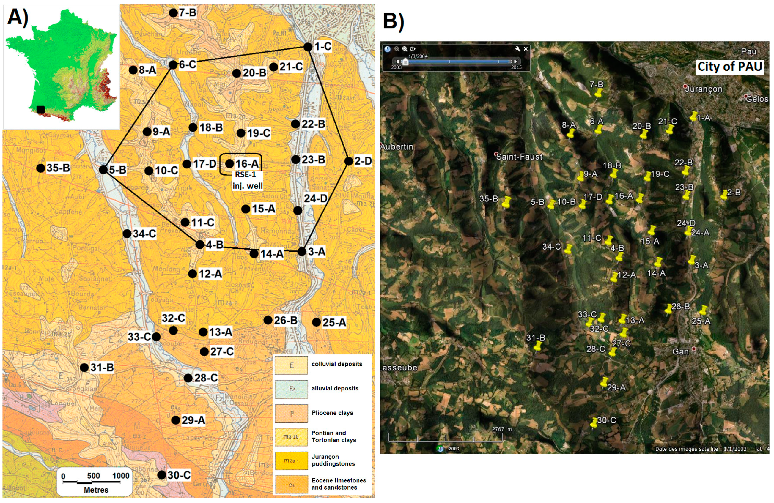
2.1. Defining the Monitoring Area

The Lacq-Rousse pilot was part of a MMV program, established by the site operator to satisfy regulatory requirements developed for this experimental project in accordance with French government requirements. Monitoring was designed according to a preliminary risk analysis and the specific configuration of the storage site (deep reservoir; thick caprock; small amount of CO2 injected; final pressure far below initial reservoir pressure; only one well intersecting the reservoir). The monitoring should provide information on site integrity, well injectivity and storage performance, as required by the French administration, and was designed to cover ten “parameters”: (1) continuous monitoring of the injected CO2 stream, (2) pressure and (3) temperature monitoring along the injection well, (4) microseismic monitoring in six dedicated geophysical monitoring boreholes (Figure 1—points 1 to 6), (5) periodical monitoring of surface water and (6) groundwater quality, as well as (7) of biodiversity of the ecosystems [31]. Monitoring of (8) soil-gas concentrations and (9) soil flux is part of site-integrity verification, aimed at addressing leakage detection, adverse effects on the environment, and assessment of the safety and integrity of the storage complex in the short term. The surveillance network set up and used during the 2008–2015 period was intended to monitor the natural geochemical background and to act as a warner in case the thresholds of natural CO2-flux concentration levels and their variability were exceeded. Last, (10) particular attention was paid to social aspects, as the area is urbanized and sensitive to environmental aspects since the start of natural gas exploitation from the Lacq reservoir in the 1960 s [28,38]. The importance of considerations on social acceptance is now well established as being one of the key parts of CCS projects [39].
When the project was designed, monitoring with remote technology of a large geographical area—several square kilometres—was not really feasible with sufficient confidence and at a reasonable economic cost. It was thus decided to focus the geochemical surface characterization on selected locations that could be regularly monitored. The surface projection of the Rousse reservoir (close to 4 km2) is included in the hexagon figure around the geophysical monitoring boreholes (1 to 6, Figure 1). The CO2 was injected at the RSE-1 borehole near monitoring point 16A (Figure 1). A much larger area was used for surface measurements, including 35 monitoring locations (36 measurement points; Figure 1) selected by the site operator in accordance with the authorities. These 35 locations lie on a 7 × 5-km grid southwest of Pau City and mostly in the Jurançon hills, which have a steep topography so that the points range in height from 180 to 350 m a.s.l. (mean elevation of 270 m).
The locations remained the same throughout the entire project period, and were chosen to be representative of the local geological context as known from previous geological and geophysical work, and to largely exceed the surface projection of the storage reservoir. The monitoring points were also selected in locations that could remain the same throughout the monitoring period, as the region contains many vineyards and other agricultural plots (corn fields and pastures). Additional information and discussion on the representativeness of such a geographical coverage is given in [35].
The number of monitoring points results from a compromise between the operator’s point of view, oriented towards a best fit between costs and benefits to ensure storage integrity, and the scientific point of view that might have required a larger number of monitoring locations to establish a more statistically reliable database. A third aspect to be considered was public acceptance of the Lacq-Rousse pilot at the time the project was launched, as some opposition existed to the project [31]. The site operator insisted that surveillance should occur at well-defined locations, the access to which is managed through specific agreements with each landowner. No other monitoring points could be created. Consequently, the 35 sites pre-selected in spring 2008 were first surveyed in September 2008 to define the exact location of measurement points, and then surveyed during subsequent data acquisitions.
The monitoring points cover six different geological units. Most measurements were made in the Jurançon hills ‘puddingstone’ (7 points; m2a-l on Figure 1), Pontian to Tortonian clays (9 points; m3-2b) and alluvial deposits (10 points; Fz). Other measurements were located over Eocene limestone and sandstone (5 points; e4), Pliocene clays (3 points; p) and colluvial deposits (2 points; E). These 35 locations were monitored as part of an evolutionary scheme:
  • Six baseline measurement campaigns, from September 2008 to December 2009, were done quarterly as required by the MMV plan, including the September 2008 campaign that was initially designed to select the monitoring locations and thus is only partially included in the database used for defining baseline values.
  • Measurements during the CO2 injection period (January 2010 to March 2013) were set by the site operator at two sessions per year, one at the end of fall and the other at the end of winter. Seven campaigns, referred to as “low season” campaigns, were carried out during this phase. In order to complete the dataset, other data acquisitions—not required by French law—maintained the quarterly frequency of data acquisitions. Funding for these two additional campaigns was obtained from a related research project, leading to four additional “high season” campaigns in spring and summer.
  • Finally, post-injection monitoring (March 2013 to December 2015) was restricted to “low season” data acquisitions performed three times as required by French law.
Site measurements thus took place from September 2008 to December 2015, resulting in a dataset of 20 different campaigns available for the duration of the entire project.

2.2. Choices of the Methods: What has Been Done and What has Not

The monitoring methods considered in this paper are based on surface geochemical characterization of gas species. The way the monitoring was designed must be viewed from the perspective of what was technically and economically realistic in the mid-2000 s (overall budget of the pilot site was 60 M€ plus 3 M€ for additional research; [31]), rather than from today’s viewpoint based on then non-existing monitoring techniques and protocols [18]. Most of the surface geochemical monitoring then relied on robust methods based on spot measurements of soil-gas concentrations at 1m-depth and of soil-gas flux at the soil/atmosphere interface at regular intervals [35]. Gas flux measurements concerned CO2 and CH4 emissions on the soil surface. Soil-gas concentration measurements covered CO2, O2 and CH4. Regulatory requirements only concerned CO2 monitoring (soil concentration and flux). Other gas species which may have been surveyed (e.g., 4He; [35]) are not considered. Biases that may be inherent in these monitoring methods will affect the entire dataset, whose interpretation thus is unaffected by internal inconsistencies linked to changes of the monitoring equipment. Given the limited number of monitoring points, it is clear that no spatial integration of the data is possible. Data interpolation for locating leakage points with a high confidence level requires many more monitoring locations [40] and less than 100–200 m interspace between points for statistical soundness. With this spatial density of sampling, only small areas can be surveyed at limited scale; to date, examples rely on induced CO2 leakage in near-surface environments [27,41,42], or on the spots of natural CO2 seeps [40,41].
This monitoring scheme can be criticized especially if it is considered through the prism of knowledge today, e.g., considering the use of long-term monitoring methods or the use of methods of larger geographical coverage. Some of these methods were nevertheless used at the Lacq-Rousse pilot, being part of research applications because the feedbacks on their uses were often too limited to allow uses under regulated applications. These uses concerned:
  • The monitoring of temperature, pressure and radon activity time changes (and not CO2) at one location (Point 24, Figure 1). Nowadays, under a cost/benefit approach, the use of such continuous monitoring systems is more developed [42] but these systems were only in use by the research groups who developed them in 2007/2008 [43].
  • The monitoring of the atmosphere was done at one location (point 16A; Figure 1) by the eddy-covariance technique or by passive-infrared remote sensing [31,44,45]. Although the eddy-covariance technique was robust in the 2000s, the radius of the monitored area (1 to 2 km with a 10 m height pole) would have implied deploying numerous devices in order to monitor the entire 35 km². A single eddy-covariance system cannot detect leakage in an area it does not cover, or where the wind direction is not oriented toward the detection system. The use of such systems to locate leaks within a pre-defined surveillance area is of more recent application, relying on data from risk assessment of the plausible location of leaks [46]. The passive-infrared remote sensing system showed that the CO2 gas concentration in the atmosphere close to the RSE-1 pad was influenced mostly by photosynthetic processes and by particular wind dynamics.

2.3. Soil-Gas Concentrations

Soil-gas concentrations were measured at 1m-depth after drilling a small hole in the soil with a battery-powered drill (1m-depth, 1 cm diameter) and inserting a sampling probe (copper tube, 1 m long and 1 cm diameter). Due to land-use constraints, it was not possible to keep the sampling probe in place between each monitoring campaign, which would have been the best option. The holes were surface-capped with locally present soil. For each new measurement, probes were re-inserted after a new hole was drilled. Soil-gas concentrations were directly monitored using with an LFG20 Infra-Red Gas Analyser (IRGA—ADC Gas Analysis Ltd., UK) using low-rate pumping (200 mL·min−1) to avoid disturbing the soil atmosphere. After purging of the tubes and pipes, stable readings were reached within tens of seconds. The stability of the readings, during measurement and gas-sample collection, was regularly checked and, if necessary, the site was resampled. The analytical precision for CO2 and CH4 was ±0.5% (of the reading) at low concentrations (0.01–10% vol.) and ±3% (of the reading) at higher ranges (10–50% vol.). Oxygen precision for was ±0.4% (of the reading) in the range 0–25%. About 27% of the field measurements were cross-checked by gas-chromatography analyses at laboratory allowed determining that the overall error (sampling error induced by re-drilling + instrumental error + error on replicates) is less than 10% for CO2 concentrations greater than 8% and less than 5% for CO2 concentrations lesser than 6%.

2.4. Soil-Gas Flux

Soil-gas flux was measured using a direct method: the accumulation-chamber method with external recirculation [47], a protocol that is intermediate between the static and the dynamic methods. A 0.25 m2 chamber hermetically encloses the soil surface after which gases emitted by the soil surface accumulate in the chamber. During the measurement period (typically 3 minutes), gas accumulation is characterized by a roughly linear increase of the gas concentration inside the chamber [48]. Afterwards, the flux is calculated using the slope of the concentration versus the time regression line. The gas fluxes are expressed in cm3·min−1·m−2 STP (standard conditions for temperature and pressure). Conversion factors are for CO2: 1 cm3·min−1·m−2 STP = 0.033 mg·s−1·m−2; for CH4: 1 cm3·min−1·m−2 STP = 0.012 mg·s−1·m−2.
CO2 is detected with a Licor Li800 infrared device (detection limit of 1 ppm), which can be used for the monitoring of very low fluxes around 0.1 cm3·min−1·m−2 to very high gas emissions around 4000 cm3·min−1·m−2 with a detection limit of 0.03 to 0.5 cm3·min−1·m−2 [40].
CH4 flux was measured with the same accumulation chamber, associated with a Gazomat Inspectra infrared laser detector (detection limit of 0.5 ppm). This system permits detecting an extremely low CH4 emission level of around 0.01 cm3·min−1·m−2.

2.5. Other Field Measurements

The field measurements were completed by measuring local temperature and pressure in the atmosphere using a Kestrel handheld monitor, by measuring soil temperature at 15 cm-depth with a Pt100 thermocouple (Ecoscan, EUTECH) and by evaluating the soil-water content at the same depth. This water content is expressed as the ratio of the mass of wet soil to that of dry soil. Drying was done at 65 °C, below the normalized temperature (105 °C) required by the gravimetric method, but the water loss was regularly checked over a much longer period (minimum 3 days vs. 24 hours for the gravimetric method) and the soil was sieved so that confidence was good for this evaluation of the water content.
Atmospheric parameters allow normalization of the measured gas flux. Comparison of the soil and atmospheric temperatures gives information on the thermal influence prevailing at the time of sampling. Coupled with knowledge on water content in the upper soil horizons, it provides insights into the influences of external parameters on gas emission from soil [49] and thus on gas flux from soil to atmosphere.
Finally, a Barasol probe (Algade, France) was used to get temperature and pressure data on an hourly basis (precision: ±0.1 °C and ±1 mbar respectively). These data are used to provide local control on temperature and pressure changes and as a basis of comparison with meteorological data obtained from Pau-Uzein airport (about 10 km away). The probe was set at 60 cm-depth in the soil at monitoring point 24. The probe was installed after drilling a hole with a hand auger, and was laterally protected by a PVC pipe; it was installed so that its end was in contact with bare soil at the hole bottom. On surface, the PVC pipe was protected by a GoreTex® membrane and then covered by a thin layer of soil.

2.6. Laboratory Analyses

Carbon-isotope ratios of the CO2 soil-gas were determined on the same glass bulbs. After purifying the CO2, the gas is analysed through a thermostated chromatographic column connected to the inlet of a mass spectrometer (Gas Bench system associated with a Delta + XP mass spectrometer). The δ13CCO2 isotopic ratio is expressed with reference to the “Vienna Pee Dee Belemnite” standard (‰ VPDB). Analytical precision is better than 0.2‰.

2.7. Regulatory Aspects

The Lacq-Rousse CCS pilot was implemented under a well-constrained monitoring scheme referring to threshold values, authorized by the French administration [23,31]. Surface monitoring of soil-gas concentrations and flux is only one aspect of the 10 parameters described in the monitoring programme agreed by the French administration (Decree FR 2011-1411 and transcription of EC Directive 2009/31/CE). Like other aspects, it serves to establish that the storage at depth confines the injected CO2 and that no gas migrates upward.
As mentioned above, there is a clear distinction between the baseline data acquisitions operated over four seasons (2008 and 2009) for establishing the environmental background, the monitoring during the injection process (January 2010 to March 2013), and the post-injection monitoring (March 2013 to December 2015). The regulatory obligations of the three project phases are described in more detail hereafter.

2.7.1. Regulations Governing Baseline Monitoring

A set of gas species (CO2, O2, CH4, 4He and 222Rn for soil concentrations, CO2 and CH4 for soil flux) was regularly monitored at the 36 monitoring points. These data were used as input for defining seasonal changes in the soils overlying the detrital rock formations that originated from the dismantling of the Pyrenees forefront.

2.7.2. Regulations Governing Injection Monitoring

The baseline data were then used—in accordance with French Administration guidelines—to define threshold levels for a subset of gas species (CO2 soil-gas concentration and CO2 soil flux). The baseline data were compared with literature data in soils under a temperate climate [50,51,52,53,54,55,56]. This analysis—by the site operator—allowed for defining concentration and flux levels that can be considered as normal or anomalous ones (threshold levels); French regulations mention that the operator shall determine how information is processed. In particular, the operator determines the threshold values that enable detecting an anomaly in the environment that may be caused by a leak from the reservoir. The operator then decides if further investigations are necessary, or even if the injection process must be modified.
The thresholds were defined based on simple statistical considerations as there were little data available for defining universal threshold values that could be applied univocally to the Lacq-Rousse site. For example, in 2009, the potential leakage reported at the Kerr Farm, Weyburn oilfield, was not known [57,58], so that the criticality of threshold definition was not as clear. Nonetheless, it was agreed with the French authorities that these thresholds could be debated later and that they probably needed adaptation during the pilot experiment. The selected approach thus defined a “vigilance” mode as the mean value (M) plus twice the standard deviation (σ) of the baseline dataset (“vigilance” mode = M + 2σ), and an “anomaly” mode as the mean value plus three times the standard deviation of the dataset (“anomaly” mode = M + 3σ). The first attempts at defining the thresholds used the September 2008 to September 2009 dataset, as the December 2009 data were then thought to postdate the start of injection. The result was a set of high “vigilance” and “anomaly” levels (respectively 8.3% vol. and 11.2% vol. for CO2 concentration and 16.6 cm3·min−1·m−2 and 21.5 cm3·min−1·m−2 for CO2 flux). The operator then refined these levels by only considering the data acquired during “low season”, but this meant that the redefined threshold levels were only valid for the “low season” monitoring. This was approved by the administration. The question of what would happen if leakage was reported during the “high season” was not specifically addressed; further work would have been necessary, such as required when a threshold is exceeded during “low season”. Fortunately, soil-gas investigations and the use of a process-based method (defined as such by Romanak et al. [59], but used before) would certainly have provided sufficient evidence of the origin of the gas to reject any allegations of leakage. From analysis of the “low season” baseline data, the following cases were defined and used for data acquired during the injection monitoring period:
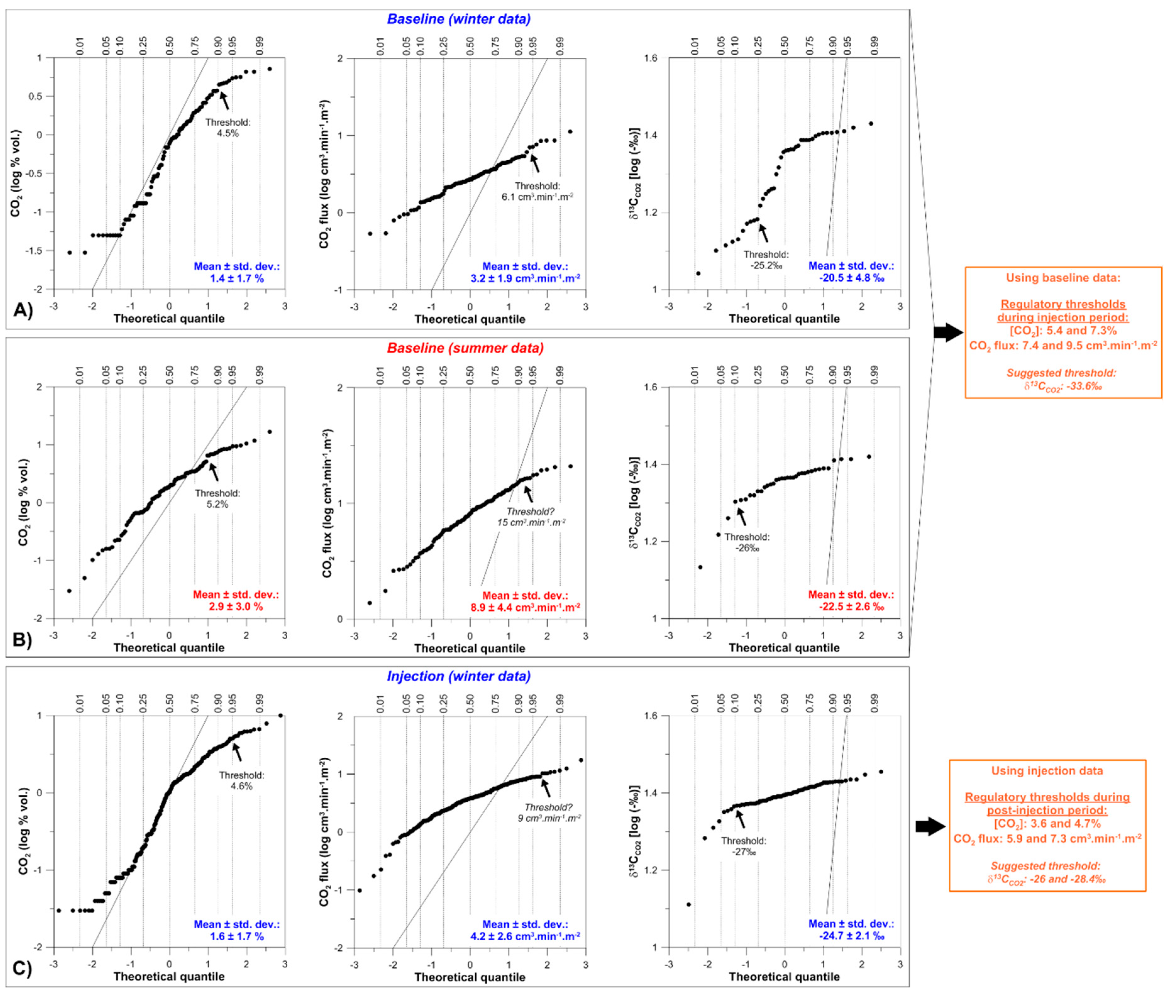
  • “Vigilance” mode (M + 2σ): This mode is activated if 5 different locations of the 35 show CO2-gas concentrations >5.4% vol. and CO2 fluxes >7.4 cm3·min−1·m−2. When this happens, the measurements are repeated to check if the threshold levels are permanently exceeded or not. The regulations did not provide for repeating the measurements, and repeat measurements were scheduled to be done during a different part of the day than the first one. If a vigilance situation occurred in the morning, the measurement was repeated during the afternoon or the day after if necessary, and if it happened during the afternoon, the repeat took place the day after. As concentration and flux are likely to vary throughout the day, measuring at different times may show whether the CO2 contribution is variable over time—probably indicating a near-surface origin—or not, and thus potentially indicating another contributing endmember.
  • “Anomaly” mode (M + 3σ): This mode is activated if 5 different locations of the 35 show CO2 gas concentrations >7.3% vol. and CO2 fluxes >9.5 cm3·min−1·m−2. Another configuration that may indicate massive leakage, is if 1 location shows a CO2 concentration >50% vol. or if the CO2 flux is >100 cm3·min−1·m−2. Regardless of how the “anomaly” mode is reached, the measurements are repeated, to check the durability of the gas signals. A soil-gas sample is also taken for laboratory measurement of the δ13C isotope ratio of the CO2. A target value of −33.6‰ was calculated as a reference, corresponding to the mean value between the mean δ13C isotope ratio measured in the soil in 2008 and 2009, and the δ13C isotope ratio of the CH4 produced by the Lacq natural gas field. This carbon-13 isotope ratio has no regulatory significance and as the δ13C isotope ratio is measured in the laboratory, there may be a delay in knowing that the threshold was exceeded. If the values are confirmed, more measurements are made at neighbouring monitoring points to determine if the CO2-level increase is confined to a small area (where the anomaly is defined), or if the increase occurs at a wider geographic scale suggesting a leak from the reservoir.
  • “Normal” mode: None of the above defined threshold levels is reached.

2.7.3. Regulations Governing Post-Injection Monitoring

The threshold levels were redefined in relation with third-party expert assessment of the injection-period data. This third-party expertise concerned the whole project and not only the soil-gas measurements, and was requested by the French authorities when injection stopped. As mentioned before, such adaptations of the monitoring protocol were foreseen from the beginning of the project, at the request of the French authorities or at the request of the site operator. The third-party expert used the soil gas concentration and flux data to calculate new thresholds. These new threshold levels were only valid for “low season” monitoring the frequency of which was reduced to one campaign per year, ideally in December. These new levels applied only to the post-injection monitoring data.
The authorities approved a new scheme. Monitoring is restricted to 35 monitoring points: the third-party expert recommended one point to be discarded as it is too frequently water-saturated and thus no monitoring of the soil-gas concentrations is possible (point 23-B, Figure 1). There, of the 10 “low season” surveys between December 2008 and March 2013, no soil-gas concentrations could be measured 5 times because of flooding, and a further 3 campaigns gave CO2 concentrations at atmospheric level. Only 2 campaigns allowed measuring a concentration well below the “vigilance” threshold (max. concentration of 1.9% vol.). Removal of this point thus had very little influence on the overall dataset.
The set of monitored gas species was reduced to the sole monitoring of CO2 and CH4 (both soil-gas concentration and flux). In addition, the acquisition of O2 soil-gas concentrations continued as the IRGA provides the opportunity to obtain this information at no extra cost.
The “vigilance” mode was redefined and is now activated if 3 different locations of the 35 show CO2 gas concentrations >3.6% vol. and CO2 fluxes >5.9 cm3·min−1·m−2. The third-party expert assessment—referring to the methodology initially used—helped calculating the new threshold level, which now corresponds to the mean value plus twice the standard deviation of the CO2 concentration and the CO2 flux measured in December 2008, 2009, 2010 and 2011 (M + 2σ). If repeated measurements show exceeding of the “vigilance” mode, a sample is taken for measuring the δ13C isotope ratio of CO2 gas in the soil.
The “anomaly” mode was also redefined and is now activated if, at a single location, CO2 gas concentration is >4.7% vol. and CO2 flux is >7.3 cm3·min−1·m−2. The thresholds were calculated from the mean value plus three times the standard deviation of the December data (M + 3σ).
An “isotopic” mode was introduced. It implies determination of the δ13C isotope ratio of the CO2 gas phase in soil for 7 monitoring points. One of these points (Point 28-C, Figure 1) was surveyed during 11 campaigns out of 13 and a good estimate of its isotope signature is available together with its variability (-23.7 ± 1.3‰). Some of the other points showed—since the start of measurements—more depleted isotope ratios together with gas concentrations over 2% vol. Therefore, for each CO2 soil-gas concentration >2% vol., a sample must be taken for laboratory measurement of this isotope ratio. The third expertise evaluated indicative levels based on the δ13C isotope ratio in the injected CO2 (−39.6‰). These suggested levels are −26‰ (“vigilance”) and −28.4‰ (“anomaly”), respectively. The site operator set its own levels at −29‰ and −31‰, respectively, but none of these levels is part of the regulatory scheme so that the values are only given as indicative.
The changes induced by this modification of the threshold levels will be discussed hereafter. As the measurements were made above a depleted natural-gas field, CH4 concentrations and flux levels were specifically checked in the soil gas and on surface. This was done to ensure that CO2 injection would not induce migration of residual CH4 from the depleted natural-gas reservoir.

3. Results

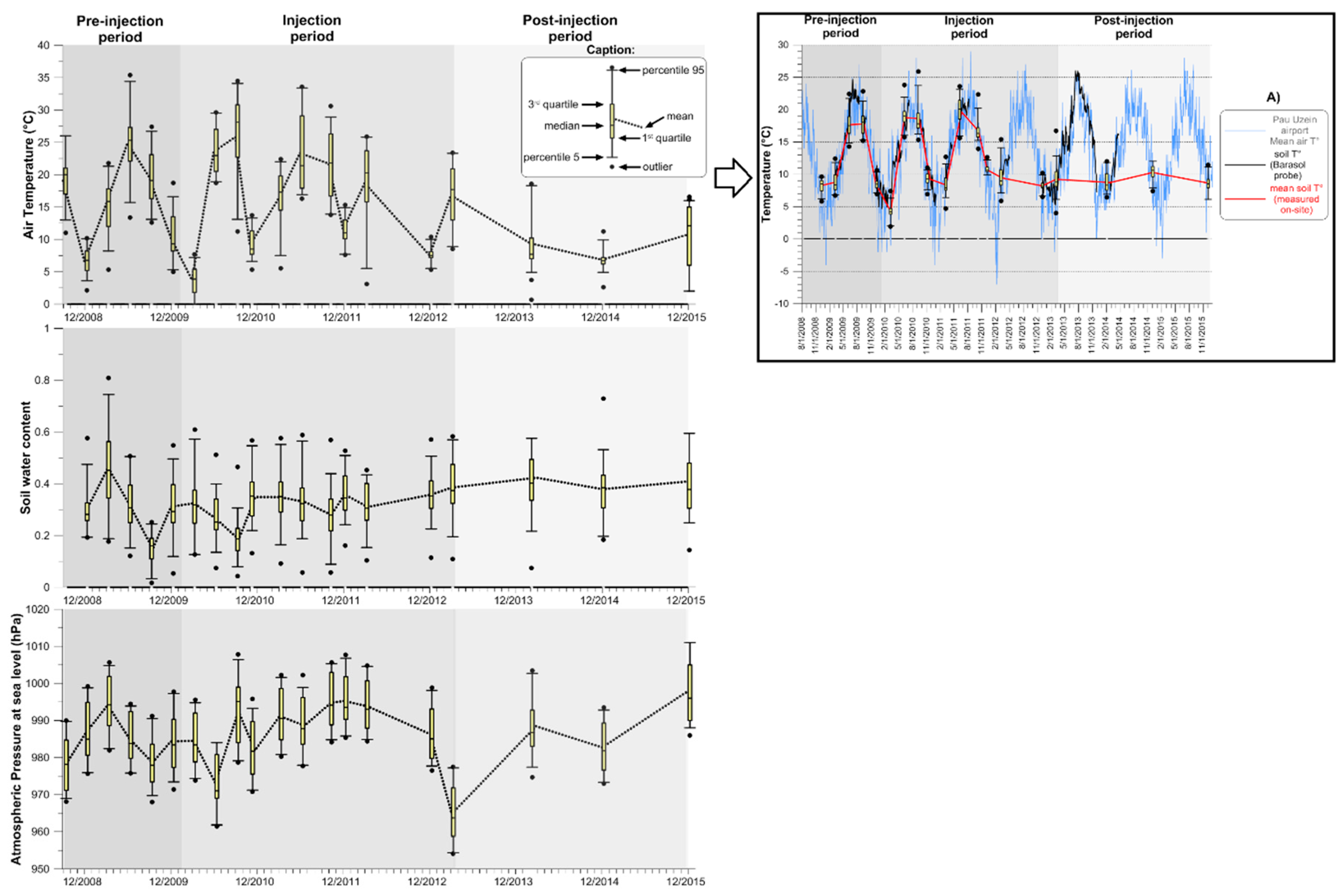
3.1. Influences of Meteorological Parameters (Temperature, Atmospheric Pressure, Rainfall)

For such long-term monitoring periods, getting a representative view of the evolution of external parameters is important. In a temperate climate, soil properties—specifically water content and temperature—can have an influence on soil-gas dynamics, especially considering the geology of surface formations (mainly detrital rocks with high clay content). Estimating the relative influence of one parameter to the other on the soil gas concentration and/or the flux and their evolutions through time, is not straightforward using the existing database. Some characteristics can nevertheless be highlighted using the dataset.
Figure 2 presents the temperature, pressure and soil water content evolutions during the 8 years of monitoring as monitored at each point during field acquisitions. The right insert details the atmospheric temperature data from Pau-Uzein airport, the data from the Barasol probe and the temperatures measured during sampling in the soil. As the thermal state of the atmosphere influences soil temperature, especially in the present case where soil temperatures were measured at shallow depth, the soil temperatures should be lower during winter than during summer, as shown by the whisker data. “Low season” soil temperatures mainly fall in a narrow range from 8.3 to 9.4 °C mean value. However, colder climatic conditions during the field surveys can cause strong temperature decreases in soil, as in March 2010 (mean value 4.3 °C); “Indian summer” conditions, on the contrary, can lead to soil temperatures over 10 °C, as in December 2012 (mean value 10.7 °C) and in December 2014 (mean value 10.3 °C). Annual climatic variations linked to the local conditions (temperate climate with oceanic influence), are thus reflected in the database, with statistically lower temperatures during winter, but these long-term trends can be overlapped by variations of higher frequency. These variations are partly linked to the geographical location of each monitoring point (e.g., hill slope oriented north and covered by trees vs. southwest oriented glade) and the time the measurements are performed.
During the 2008 to 2015 period, the mean atmospheric pressure was very close to 1015 hPa (calculated value: 1017 ± 8 hPa). The variability is higher during winter as a result of more frequent low-pressure events. Information from the pressure sensor of the Barasol probe is similar to that measured in the atmosphere (mean value close to 1021 ± 8 hPa).
Rainfall amounts and their derivate the soil-water contents were variable one year to the other (Figure 2). Generally, strong events occur in November (2009,2010,2013) with monthly amounts greater than 200 mm, but thunderstorms may lead to even larger amounts at other times, such as >250 mm in May 2013. The rainfall regime is variable because of the location of the study area, near the Pyrenees Mountains to the south and not far from the sea in the west. The result is that the general rule of winter being wetter than summer is not always true here. If “low season” monitoring pointed to water contents varying between 30 and 40%, similar values were measured in June 2009 or June 2011. However, soil-water content was generally low after summer and below 20% in September.

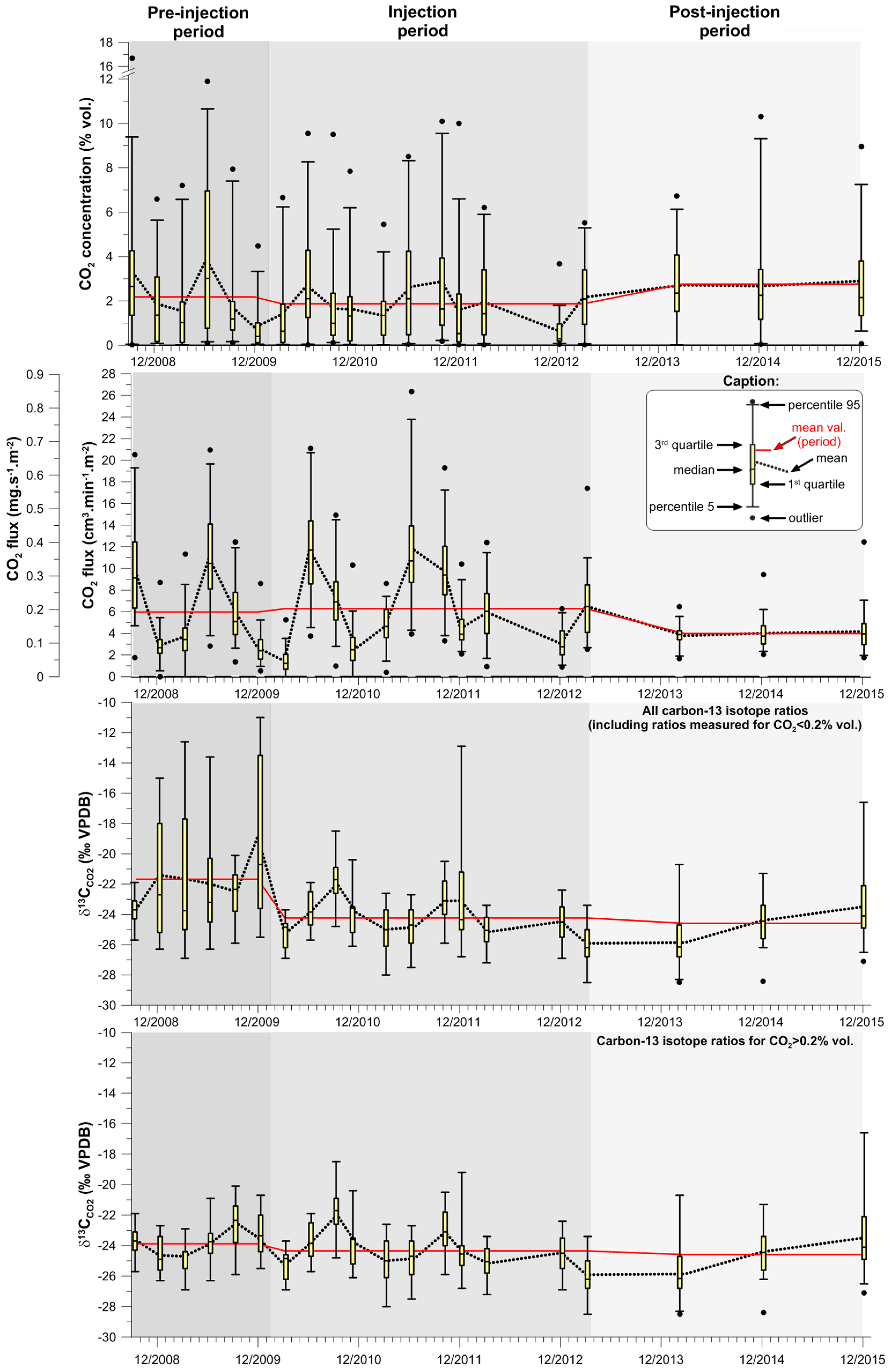
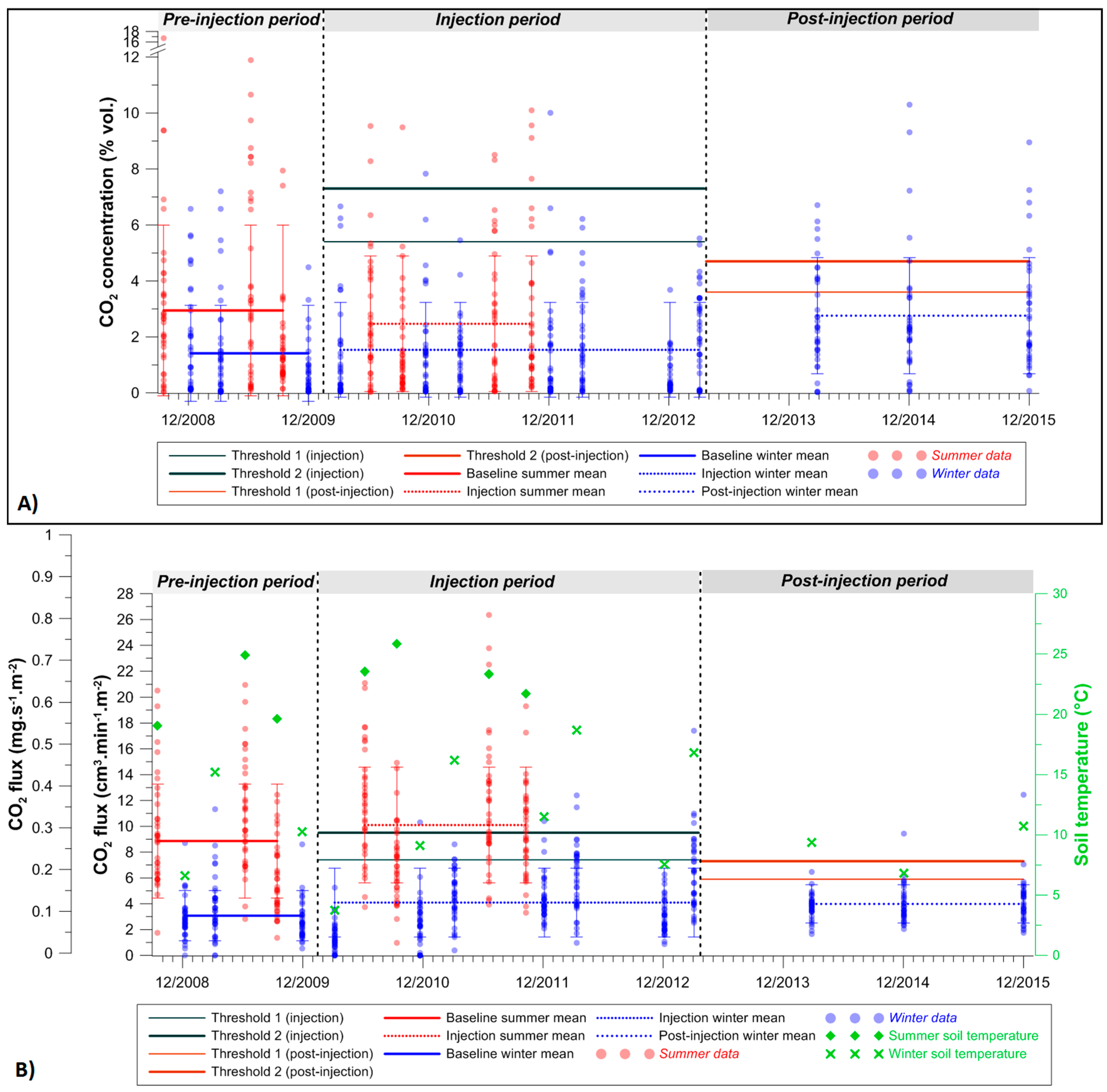
3.2. Soil Gas Concentrations—Spot Data

The distribution of data (CO2, O2 in soil gas) follows neither a normal nor a lognormal distribution. The use of Kolmogorov–Smirnov or Khi2 statistical tests always gives p-values <0.0001. The only exception to this rule is for CO2 fluxes that are likely to have a lognormal distribution (p-value of 0.271 with the Kolmogorov–Smirnov test and a p-value of 0.157 with the Khi2 test). Therefore, the use of arithmetic mean or median values, used here although not ideal, is preferred as soil-gas studies usually refer to the use of such averaging methods.
CO2 concentration changes with time are shown on Figure 3. O2-concentration variations will be discussed later in the Discussion section, together with CO2-concentration variations. A total of 710 single measurements is available for the entire monitoring period. CO2 concentrations varied from near atmospheric levels (0.03 to 0.04%) up to 16.7% (Point 24-A, September 2008). Mean value is 2.1 ± 2.2% for the whole dataset and the median value is close to 1.4%. Oxygen soil-gas concentrations ranged from 1 to 21% with a mean value of 17.8 ± 3.5% and a median value of 19%.
There are some differences between “low season” and “high season” measurements. During summer, CO2 concentrations tended to be higher (mean value 2.7 ± 2.7%; median value 1.7%; 252 data) as a result of biological and microbial activity in soils. This statement has to be balanced by reference to the temperatures and especially the soil-water contents (Figure 2). In September 2009 and 2010, soil-water contents were at their lowest levels (<30%). Soil dryness has adverse effects on soil organisms and reduces their activity. This may have led to a decrease of CO2 production in soil so that soil CO2 concentrations had low mean and median values, mimicking those measured during winter. The highest mean and median CO2 concentrations were measured when soils were warm and humid, which was mainly encountered during June acquisitions. On the contrary, winter-time acquisitions do not necessarily imply a strong decrease in CO2 soil-gas concentrations. The mean value calculated for the whole dataset is lower (1.8 ± 1.9%; 468 data), but the median value (1.3%) is relatively close to that calculated for summer months (only a 0.4% decrease in the median value). This suggests that soil biological activity decreases during winter, but that there is still enough activity to produce significant CO2 gas concentrations in soil. The influence of soil humidity on soil CO2 production was less obvious as no water stress was found during winter months. Soil temperature influenced the measurements; when they dropped below 10 °C (e.g., December 2009, March 2010 and December 2012), the soil CO2 concentrations were at very low median levels, well below 1% in volume. However, when monitoring during more clement climatic conditions, such as in December 2014 and 2015, the CO2 concentrations mimicked those of “high season” conditions (median values >2%).
Another potential variability is much more short-term: the distinction between morning and afternoon sampling is far from obvious. During one monitoring session, the routes between points were randomly chosen so there was no additional bias linked to preferential occupation of locations during the day. There certainly is a daily variation of the soil CO2 concentrations but these changes cannot be assessed with the present dataset.
The statement suggesting that the best period for site monitoring is when the biological activity is low in soils cannot be verified in the present case. Although winter is generally referred to as the best period for highlighting the presence of gas with a deep origin [55], in our study CO2 concentrations were not always at their lowest levels during winter. For example, another survey in southeast France showed lower CO2 mean concentrations during spring or summer [60]. It is thus of crucial importance to have other markers (monitoring of other gas species and/or isotope data) in order to correctly attribute gas concentrations to surface processes or to other origins.
Monitoring of methane using IRGA was not informative (no deviation of the reading) but the cross-checking measurements done at the lab by gas-chromatography allowed us to detect very low amounts on some samples (66 of 195 samples). Minimum and maximum concentrations were 2 ppm (instrumental detection limit) and 13 ppm, respectively, compared to the 1.8 ppm concentration of the atmosphere. Mean and median values were 3 ± 5 ppm and 2 ppm, respectively. CH4 detection in soil was rather infrequent for most points. Of the 36 monitoring points, 10 points never showed detectable CH4 concentrations, including point 16-A close to the injection borehole RSE-1, and for eight further points CH4 was only monitored once, including point 17-D close to the other borehole reaching the former CH4 reservoir. However, CH4 was measured 10 times at points 1-C and 28-C, and 8 times at point 24-A; for these three points, there was no apparent relation with time, i.e., no increase of CH4 concentration that could to be related to the CO2-injection process. The hypothetical origin of this CH4 will be discussed in Section 4.

3.3. CH4 and CO2 Gas Flux

CH4 flux was searched for in parallel with all CO2-flux measurements, but none exceeded the instrumental detection limit (0.01 cm3·min−1·m−2). This agrees with similar measurements in normally drained European soils [51]. CH4 flux was thus considered as insignificant.
CO2 flux changes over time are shown on Figure 3. A total of 717 single measurements are available for the whole monitoring period. CO2 flux varied from 0 up to 26.4 cm3·min−1·m−2 (Point 4-B, June 2011). Mean and median values for the whole dataset were 5.8 ± 4.2 cm3·min−1·m−2 and 4.4 cm3.min−1.m−2, respectively. These values are in the upper range of bibliographic values for biological flux in the European temperate climate zone, outside any known geochemical anomaly and on a normally drained soil (flux less than 4 cm3.min−1.m−2 [51]; flux up to 14 cm3·min−1·m−2 [61]).
However, the recent analysis of the biogenic CO2 and CH4 emissions data in France (24 various natural sites, more than 2600 measurements) shows that the most probable CO2 flux ranges are respectively from 0 to 6 cm3·min−1·m−2 in winter and 3 to 20 cm3·min−1·m−2 in summer. The average values are respectively 2.7 cm3·min−1·m−2 in winter, and 9.3 cm3·min−1·m−2 in summer and 5.8 cm3·min−1·m−2 for all seasons’ data [62].
CO2 gas flux measured between 2008 and 2015 on the surface of the Rousse site are mostly in the high range of this all reference flux, because they were measured on very fertile land in the oceanic climate of SW France that is characterized by hot and wet summers and mild winters.
Regardless of the measurement period, the ratio between highest and lowest measured values is always highly significant. Here it was 4 to 60, without considering zero-flux measurements, but the same observation is made on reference sites and is due to the heterogeneity of biological activity and to the permeability of soil to gas.
Quarterly measurements from September 2008 until March 2012 highlighted a clear seasonal variation of the gas flux between summer and winter conditions (Figure 3). Mean CO2 flux values in June or September (6 to 11.8 cm3·min−1·m−2) were always higher than those in December or March (1.4 to 5.9 cm3·min−1·m−2). The same trend was observed for maximum and minimum values, except in one case: zero-flux and values close to zero occurred only in winter, when soil biological activity is low, or rain can saturate soil porosity with meteoric water, causing reduced permeability. The observed seasonal variation of the gas flux is well-known when measuring CO2 flux from biological origin; it is due to natural changes throughout the year of bacterial and root activity in the soil.
No significant difference of gas flux was observed between the baseline study from September 2008 to December 2010, and the injection period from January 2010 to March 2013. During these two periods, CO2 flux followed the expected seasonal pattern, without any significant deviation. The mean values measured during the baseline-study and the injection periods were almost the same, about 6 cm3·min−1·m−2. During the post-injection period, three field campaigns took place in winter; the mean value was about 4 cm3·min−1·m−2, which was very similar to the flux measured in winter during the baseline and the injection periods.

3.4. Carbon-Isotope Ratios of Soil-Gas CO213CCO2)

A set of 260 carbon-13 isotope ratios was determined from September 2008 to December 2015 (Figure 3). One location (point 28) was monitored each time in order to evaluate the temporal changes that may affect isotope ratios. δ13CCO2 isotope ratios ranged between −11‰ and −28.5‰ VPDB, with a mean value of −23.5 ± 3.1‰ and a median value of −24.2‰. These mean and median values fall well within the field of carbon-isotope ratios originating from soil biological activity in a temperate climate. These ratios are more depleted than those reported for the sole baseline acquisitions. An average ratio of −20.6‰ was at that time calculated for five campaigns between December 2008 and December 2009, thus excluding the first campaign in September 2008 [35]. As the sampling strategy during injection and post-injection monitoring was oriented to the sampling of points with a significant CO2 concentration in the gas phase, biases linked to the dilution of soil air with low CO2 concentration by atmospheric CO2 were therefore reduced, as will be discussed later.

4. Discussion

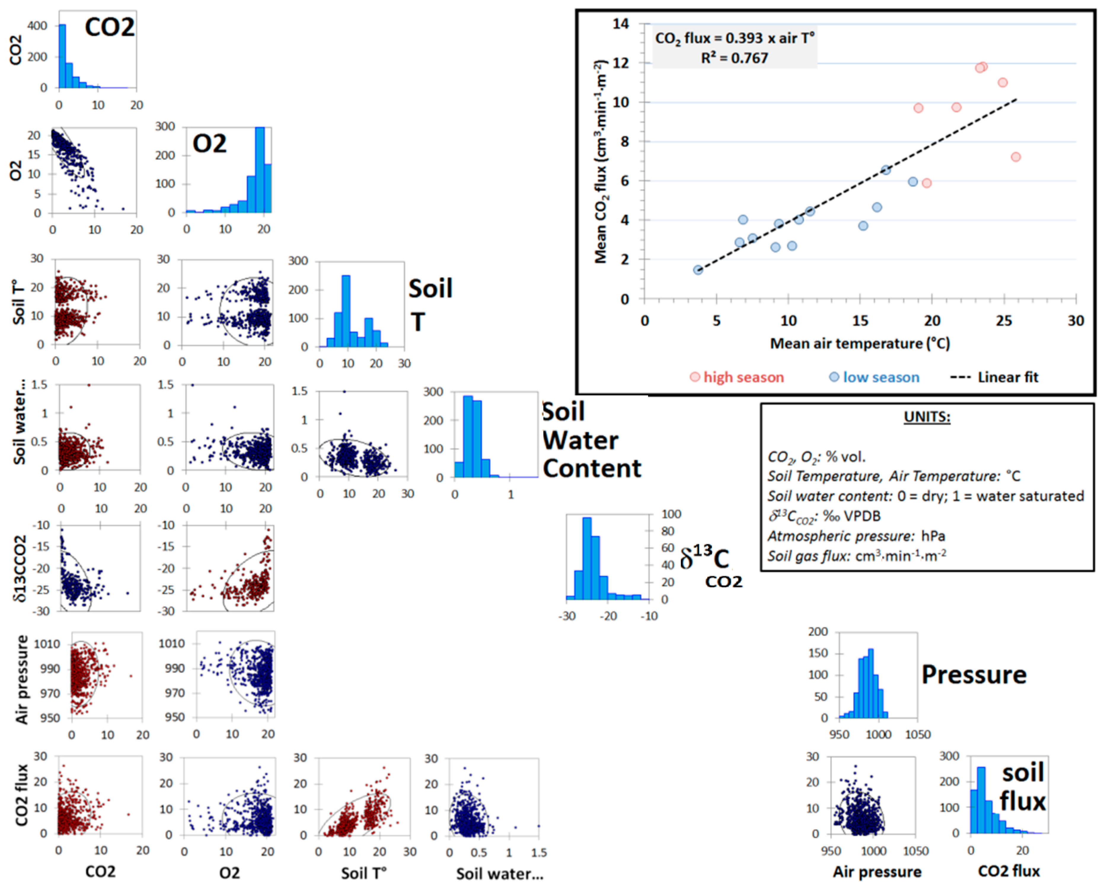
4.1. Relations between Parameters

The results presented in the previous sections indicate that the variability of soil-gas concentrations or CO2 soil flux is mainly related to annual seasonal changes. The whole dataset can thus be considered in terms of time-related changes, suggesting that such changes are unrelated to the CO2-injection process. This agrees with the baseline data [35]. Figure 4 shows some of the relationships between gas phases and external parameters.

4.1.1. Influences of Temperature, Pressure and Soil Water Content

Plots representing soil temperature as a function of CO2 and O2 have the same shape. Two groups exist, one corresponding to “low season” data acquisitions, with soil temperature around 10 °C and less, and the other corresponding to “high season” data with a higher temperature (over 15 °C). When the data are considered as a whole, the relation between soil-gas concentrations and the soil temperature is masked: e.g., CO2 concentrations around 10% were monitored during both winter and summer. This is not contradictory with previous statements (see Section 3.2) that have established the mean CO2 concentrations were lower during the “low season”. This is only the result of considering the entire dataset in which local effects (topography, soil temperature, soil water content) are hidden. When the data are considered more in detail, the influence of temperature can be highlighted, e.g., for CO2-flux measurements that show a tendency to be higher when the temperature is higher (inset in Figure 4). Flux equal to zero is often measured during winter, when the soil temperature is only a few degrees Celsius and the air temperature hovers around 0 °C. Depending on the soil biological activity, gas flux is generally higher during “high season” but high flux, over 10 cm3·min−1·m−2, may be measured locally during the “low season”. This illustrates the effect of thermal draw on gas exchanges between soil and surface.
At the opposite, the relationships with pressure or with soil water content (Figure 4) are non-informative in the present case study.

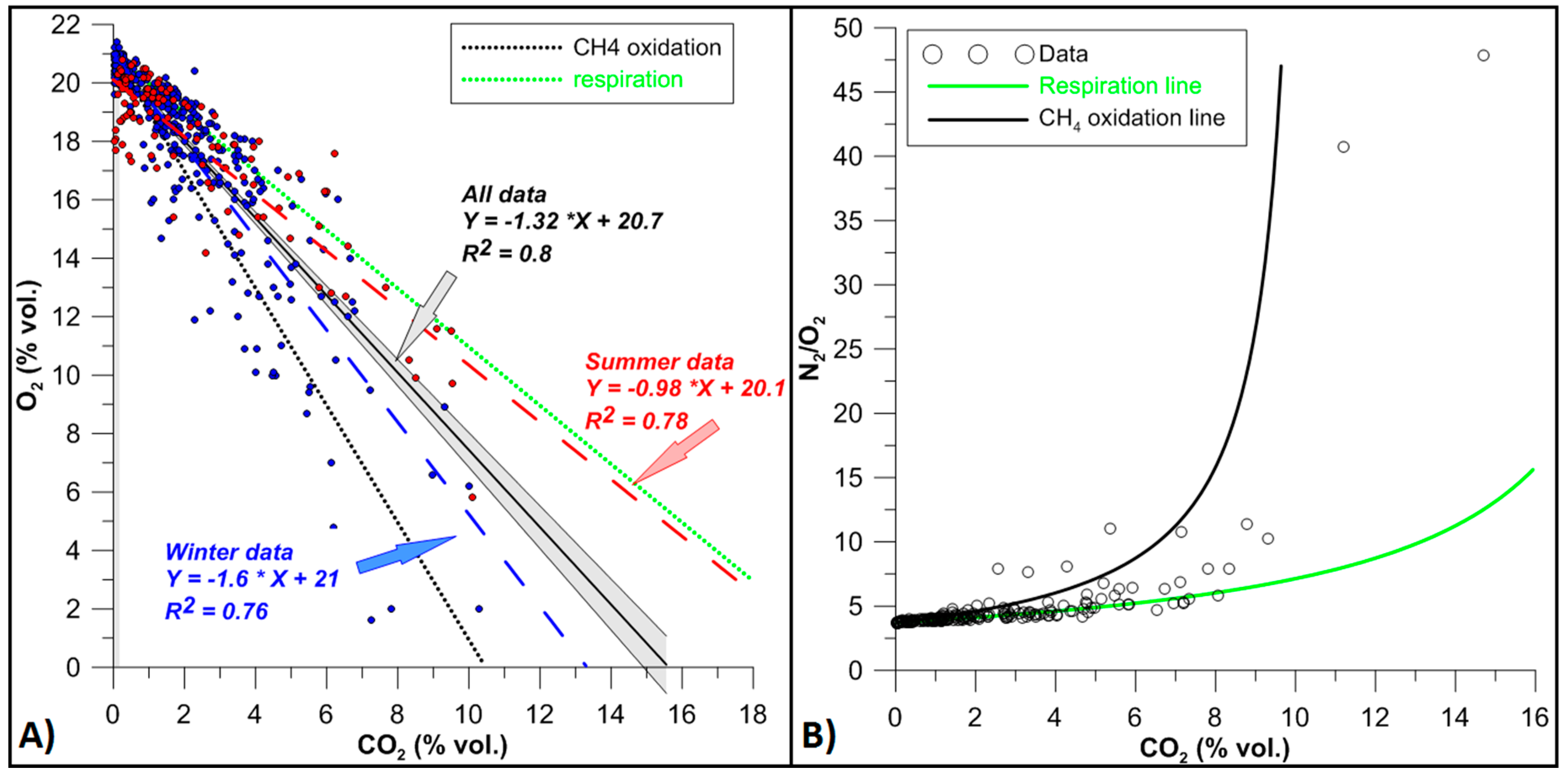
4.1.2. Relationships between Gas Species

As part of a “process-based approach” [60], the relationship linking CO2 and O2 soil-gas concentrations (Figure 5) is the most frequently used. There is a strongly inverse correlation between CO2 and O2 (O2 = 20.7 − 1.32 x CO2; R2 = 0.724), a rise in CO2 being balanced by a depletion in O2, though the slope of the regression line is not equal to −1. The ratio of −1 would suggest that each appearance of 1 CO2 mole induces the disappearance of 1 O2 mole (pure respiration process: CH2O + O2 = CO2 + H2O; in green on Figure 5A). The regression line calculated for summer acquisitions (“high season”) points to a slope close to –1 and thus points to a dominant influence of the respiration process in soil to account for the CO2/O2 relationship. The CO2/O2 relationship during winter (“low season”) has a different slope of −1.6 (Figure 5A), closer to that of the CH4 oxidation line (CH4 + 2O2 = CO2 + 2H2O; in black, Figure 5A).
Some “high season” data have CO2 concentrations >2% vol. and plot above the respiration line (i.e., slope less than 1), in an area where the CO2 concentration in gas rises with only minor depletion in O2 (CO2/O2 ratio <1). Such behaviour may correspond to the influence of exogenous CO2. The presence of CO2 from mantle/crustal origin is unlikely; such seeps from depth are not reported locally – mineral waters circulating at depth are N2-rich and depleted in CO2. The presence of naturally occurring CO2 from the Lacq reservoir, or of CO2 resulting from the injection process, is not compatible with carbon-13 isotope data. The origin of data falling above the respiration line thus remains unclear, but may be due to specific processes occurring in soil in late summer, when soils are under hydric stress.
Some data, especially during the “low season”, may show some link with the CH4 oxidation line, or with processes such as pyrite oxidation [63] that deplete the O2 with a CO2/O2 concentration changes ratio >1. Nevertheless, pyrite oxidation was discarded during the baseline acquisitions [35], as this mineral is uncommon within the detrital sedimentary formations. Information from the N2/O2 ratio vs. CO2 concentrations plot [59] given on Figure 5B also suggests CH4 oxidation may have some contribution for some measurements, albeit the main driver of CO2/O2 concentration changes in soil remains respiration processes.
As mentioned before, no CH4 flux was measured but some soil gas measurements did point to the presence of a few ppm of CH4. The presence of CH4 at concentrations over the atmospheric concentration is not common, as most soils in a temperate climate show CH4 oxidation in the soil column [64,65]. Natural leakage from the former CH4 reservoir may thus be the culprit, even though no isotope ratios were measured (δ13CCH4 and δDCH4) to clearly attribute a CH4 origin. Methane concentrations of a few tens of ppm are likely to be found in faulted areas (vertical migration of CH4; [66]) but deep-rooted faults are not known to affect the thick sedimentary pile of molasse formations [31,67]. Methane emission to the atmosphere can also occur as a purely diffuse mechanism [68] to form the so-called CH4 micro-seepage, defined as the slow and continual loss and upward flux of CH4 and light alkanes from depths of 2–5 km in sedimentary basins [69]. Methanotrophic oxidation processes in soil consume CH4 and lead to non-existent or negative CH4 flux at the soil/atmosphere interface – this is congruent with our observations (no CH4 flux).
The occurrence of such seepage is yet unproven and seems hypothetical in view of other information. Reactional processes can consume methane, but this is unlikely for helium. The Lacq-Rousse reservoir is 4He-rich (65 ppm; [67]), and if micro-seepage occurs then 4He will also diffuse and, as a chemically very stable gas, should be detected in the soil. No 4He enrichment is reported in soil gas (unpublished data) neither in a local aquifer sampled near injection well RSE-1 [31]. This aquifer has also very low concentrations in dissolved CH4 (10−8 mol·L−1 when measurable; unpublished data) and the supply of CH4 by the aquifer is highly unlikely. Natural micro-seepage from the reservoir is thus not certain and it must be assumed that the presence of CH4 is rather linked to surface biological processes in non-anthropogenic soils. The fact is that soil CO2 seems to be dependent from production through CH4 oxidation in winter during periods of lower biological activity in soil. This effect vanishes—or is non-existent—during period of higher CO2 production from biological processes in soil during summer.
The relation between CO2 as soil gas and CO2 as soil flux is presented in Figure 4. Baseline data did not highlight a relation between concentration and flux, only a slight positive tendency for “high season” acquisitions [35]. The situation did not change during injection and post-injection monitoring. “Low season” measurements are strictly uncorrelated (R² = 0.006; 458 data) and “high season” ones are barely correlated (R² = 0.018; 252 data), but this may be only related to the number of data that is smaller for summer acquisitions. There is no correlation between CO2 flux and CO2 soil-gas concentrations, suggesting a near-surface origin of the CO2 gas (no CO2 flux from the storage reservoir and only CO2 production in the soil). In addition, this highlights the poor vertical connectivity of the soil, probably due to high clay-mineral content.

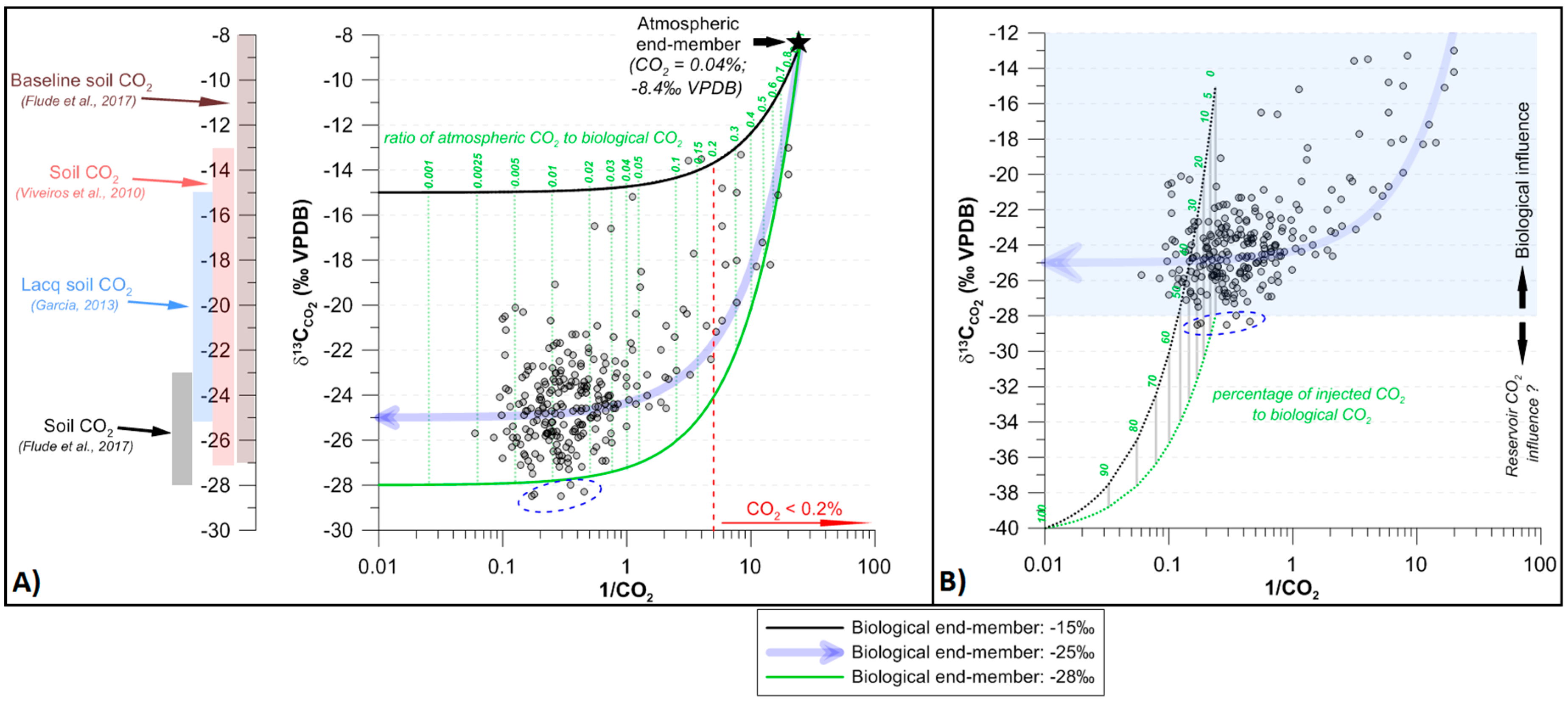
4.1.3. Carbon Isotope Ratios (δ13CCO2)

Another way to infer the origin of the CO2 gas phase is to refer to carbon-13 isotope-ratio determinations (Figure 6). As shown during the baseline site characterization, carbon-isotope ratios mainly fall within a range of −19 to −28‰ VPDB. A larger range was established by Garcia [70] (−15 to −25‰). The −19 to −28‰ range is the result of CO2 isotope equilibration with that of biological organisms in the soil under steady-state conditions [71] and more specifically the equilibration with vegetation whose photosynthetic cycle produces molecules with three carbon atoms (Calvin cycle). Molecules produced under the Calvin cycle have carbon-isotope ratios ranging from −21 to −33‰ [72] with a mean value of −27‰ VPDB. The CO2 produced from these molecules is enriched by a factor close to +4.4‰ [73], leading to δ13CCO2 ranging from –17 to −29‰, the most common values in a temperate climate being near −22 to −25‰ [74] with possible extension to more depleted ratios (down to −28‰; [75]) or to more enriched ratios (up to –13‰; [76]). Applied to our dataset, this suggests that the presence of CO2 in soil over the Lacq-Rousse storage site is essentially the result of natural biological processes occurring in soil.
If the CO2 were produced from the remaining CH4 in the storage reservoir, it should have a lower δ13CCO2, as equilibration with CH4 having a lower δ13CCH413CCH4 of the Lacq-Rousse field: −41 to −43‰ VPDB; [67]) will produce depleted δ13CCO2 [75]. Similarly, the injected CO2, produced by CH4 oxy-combustion, has a δ13CCO2 of −40‰ [67]. Although some re-equilibration and/or dissolution processes in water may occur in a 4500-m-thick sedimentary pile, it is very unlikely that the monitored carbon-isotope ratios of the CO2 originate from the storage reservoir. A difference larger than 10‰ between injected CO2 and baseline CO2 is recognized as representing favorable conditions for the use of carbon isotope ratios as a tracer [77]. The hypothesis of CO2 originated from the reservoir is tested in Figure 6B for the five samples having ratios lower than −28‰. The isotope composition of the CO2 that may originate from the storage is taken at −40‰ and mixing with soil gas is calculated (using the −15‰ and −28‰ endmembers). Three samples are outside binary mixing relations – to plot under such relations, the soil gas component should have a ratio more depleted than −28‰ – founding such a depleted ratio in soil is very unlikely. Only two samples may plot on a binary relation between CO2 from the storage and CO2 from the soil (at −23‰) but this is not in agreement with other data. Analyses of noble gases in soil gas highlight the presence of atmospheric endmembers (neither 4He nor 84Kr enrichment), whereas the gas phase from the reservoir has a very different noble-gas signature [70].
Nevertheless, some δ13CCO2 ranging from −18‰ to −11‰ VPDB are not explained—or are partly explained—by the previous statements; they are less depleted in the heavy isotope (13C) than the majority of the data. Such deviations may be attributed to contamination by atmospheric CO213CCO2 of −8.4‰; [78]) at least for data that plot close to the dilution lines reported in Figure 6A and that have low CO2 concentrations (<0.2% vol. i.e., 1/CO2 >5). Under 0.2% of CO2, the atmospheric endmember has a contribution that may become significant as may be deduced from the relative contribution of soil CO2 and atmospheric CO2 reported on Figure 6A. Such contamination was mainly stated during winter acquisitions (2/3 of the data) and may result from sampling bias linked to defective sealing of the sampling probe or the presence of water in soil that hampers the correct pumping of soil gas (half of the anomalies are from the December 2009 campaign). Hypothetical mantle or the lower crust CO2 degassing (δ13CCO2 ranging from −4 to −8‰ VPDB; [79]) is not supported by 4He measured values. Finally, CO2 produced by the dissolution of carbonate rocks or soil carbonates will have a δ13CCO2 around 0‰ VPDB and a contribution of carbonate dissolution may also explain part of the low depleted data but this hypothesis cannot be tested using our data.
Scattering of the δ13CCO2 data is strongly reduced when low CO2 data are filtered from the measurements (Figure 3). There was only little variability throughout the monitoring period: the mean baseline value is −23.9‰, the mean injection value is −24.3‰ and the mean post-injection value is −24.6‰. The apparently progressive decrease of ratios that is observed when using the whole δ13CCO2 dataset is thus the result of more frequent atmospheric contamination of the samples during the first sampling sessions, as no selection based on CO2 concentration was made. The selectivity used afterwards, especially during post-injection acquisitions (CO2 >2%), strongly limits this risk.
In conclusion, the data provided by carbon-isotope ratio measurements point to a near-surface biological origin for CO2 gas in the soil, and thus to CO2 flux at the soil/atmosphere interface.

4.2. General Discussion

4.2.1. Monitoring Strategy—The Aims

Geochemistry, including surface and near-surface investigations, is one of the many tools available for CCS site monitoring [37,80] and was extensively used at the Lacq-Rousse CCS pilot [23]. Among these investigations, soil-gas monitoring–concentration and soil flux measurements—was implemented under a scheme approved by the French administration. Soil-gas monitoring is a major geochemical tool for detecting gas micro-seepage from geologic sequestration [81] and should be included in MMV protocols [18]. A key parameter about the impact of leakage from deep storage formations, commonly discussed in recent years, was highlighted by Jones et al. [82]: “The impacts from many lower level fault—or well—related leakage scenarios are likely to be limited spatially and temporarily and recovery may be rapid”. However, Beaubien et al. [83] stated that “leakage detection can be complicated by the natural background of near-surface gas geochemistry and by its variability as a consequence of temporal, seasonal, geological, biological … changes”.
Consequently, each near-surface strategy for gas monitoring is site specific and must be thoroughly evaluated in order to provide reliable information during the injection and post-injection periods. The definition of baseline monitoring is important [37]. Once injection takes place, no reverse process exists for determining background levels of soil gas. Even if no leakage occurs, detractors may argue that the storage formation could have experienced some changes after which it has become difficult to prove site integrity. The controversy about the Weyburn field and the allegations of leakage after gas injection illustrate the importance of correct baseline measurements, even though in this case seepage allegations were dropped in the light of data and methods that were not specifically considered during baseline, if any, data acquisitions [57,84].
The soil-gas monitoring of the Lacq-Rousse field relies on these facts. The initial ideas in 2006 for this work focused on studying the feasibility of the pilot itself, but the importance of a correct design of the baseline monitoring and its strategy became rapidly clear and was adopted in early 2007 when the European Directive 2009/31/EC was not yet operative. This matched French regulatory requirements as well as requirements of the site operator. Compared to, for instance, the Weyburn area [84], the Lacq-Rousse site has a hilly relief (slopes of 15% are common), even though hilltops culminate at only +360 m above sea level. This had a direct effect on monitoring: valleys are more accessible and have a thinner sedimentary succession than hills. A third of the monitoring points were thus located in valleys as they may be earlier affected by CO2 leakage.
The monitoring locations covered the whole surface projection of the storage reservoir and were equally distributed around the CO2 injection well. Their number is higher near the surface projection of the reservoir and includes locations on topographic highs. Six wells (locations 1 to 6, Figure 1) were drilled for seismic monitoring. As they might represent potential leakage pathways [82], some monitoring points were located close to these geophysical boreholes. Similarly, the injection well (point 16) and a former CH4 exploitation borehole (point 17) were surveyed as well. In order to consider the geological structure of the Pyrenees forefront, some points covered different geological units, such as to the south of the reservoir. Although their number is low, these points are near outcrops of deep-rooted geological units whose internal discontinuities may affect horizons lying 2000 to 3000 m above the storage reservoir at a depth of 4500 m.
Finally, the baseline characterization was done at high frequency albeit not continuous [82]. It is established that leakage is easier to detect during winter, when biological activity is low [55]. In summer, potential CO2 leaks may be hidden by high CO2 production in soil by biological processes. Nevertheless, summer baseline data allow an evaluation of the natural variability of soil-gas signals, which can be large [37,82,84].

4.2.2. Monitoring Strategy—Ways of Improvement

The surface monitoring of the Lacq-Rousse pilot site does not pretend to be exhaustive. It is part of a larger-scale project that was entirely funded by the operator, which is not so common [17]. It should be mentioned again that the French Administration approved all operations at the time the actions were planned, when these operations were considered to provide sufficient information to ensure storage safety and conformance. However, since those days progress has been made in several fields of knowledge that merit further discussion.
The first field concerns the use of monitoring mostly restricted to characterization of the CO2 phase in the near-surface environment, using a spot-sampling approach. Gas-source attribution techniques [85,86] rely on complementary gas phases to account for the specificities of the CO2-gas phase (non-uniqueness of the source, ability to interact with water, etc.). Similarly, the use of methods with a wider geographical coverage and/or allowing continuous monitoring is commonly included in compliance monitoring [18].
The second field concerns the restricted number of monitoring locations. Site selection was based on several technical factors, but also on the cost of the monitoring actions, using the ratio ‘number of locations’ to ‘information collected’ as an economic parameter. The will to deploy several monitoring points per monitoring site, which enhances scientific relevance, did not match this economic constraint. Today, conformance monitoring would certainly refer more to the use of continuous monitoring and the use of systems surveying the atmosphere [37].
Other fields of potential improvement concern the lack of monitoring deep aquifers, if present close to the injection site, or the absence of monitoring of mineral-water sites at a larger geographical scale. Some local mineral waters that are of sulphide type, such as Eaux Chaudes or Eaux Bonnes [87]. CO2 intrusion in water has a direct effect on pH and delayed effects on water mineralization, especially in the case of mineral waters that naturally have low CO2 content.
A final field in which progress has been made concerns the planning of monitoring sessions, particularly the focus on “low season” (winter) monitoring, recommended by Klusman [55] and others, leakage certainly being independent from climatic conditions. The way baseline data were used for computing initial threshold levels and the way data from the injection period were used for defining new threshold levels are also questionable. This last point is discussed in the next section.

4.2.3. Are Baseline Acquisitions Important?

Soil-gas and soil-flux monitoring during summer and winter times showed that major changes can occur from one year to the next at the study site [35]. Changes of mean CO2 concentration and mean CO2 flux between winter and summer were from 200% to 280% (Figure 7). This situation continued during the injection period with changes ranging from 160% to 240%. At the opposite, the mean values during the same season (winter/summer) were less variable: e.g., winter CO2 concentrations and fluxes only varied between 15% and 30% from baseline to injection periods. The fluxes remained at similar mean values during the post-injection monitoring albeit the soil CO2 concentrations were higher. An evaluation of the dispersal of soil-gas concentrations and fluxes is then important for obtaining sound threshold values, but the validity of the latter over long periods should be questioned. Biological activity varies throughout the year and from year to year, because of variable rainfall, variable climatic conditions, or changes in land use. This is well illustrated for soil CO2 flux and soil temperature (Figure 7B). In the present study, data acquisitions before the injection period extended over 18 months, which is in line with hydrogeological methods that consider a similar period for defining the natural variability of water resources.
The resulting dataset showed strong variability over this initial monitoring period, but the data were nonetheless used by the site operator for defining the geochemical thresholds as approved by the French authorities. This dataset provided a good description of the soil-gas behaviour over several seasons, as it showed that soil-gas and soil-flux variability may be high from one point to the next and between campaigns. Such evaluations of the natural variability are important, if only for demonstrating that each CCS site has its own characteristics and its own degree of variability. Comparison with data from the Weyburn site [83] shows that the amplitude of CO2 concentrations, or flux, is only similar to that of Lacq-Rousse during summer, and that monitoring in September or October gives much lower values as a whole.
It is thus very important to evaluate the amplitude of natural changes that can occur in a future storage site, and this not only for future checking of site conformance, but also for public acceptance as people may be opposed to CCS [88,89]. The presence of a surface monitoring network that is used at regular intervals or, even better, for continuous monitoring, is intrinsically reassuring for people living in the area of interest [37]. Its geographical coverage may not be sufficient to detect leaks, but since it exists it gives precious information on gas emissions at the surface. It will also provide control data for future use in case of deviations noted by third parties, by simply showing how the ecosystem constantly evolves.
The ultimate questions are the obligation of getting baseline data and the pertinence of surface geochemical monitoring. The Weyburn example shows that leakage allegations can be disproved even if baseline data are lacking or insufficient [58], but feedback from the US shale-gas industry shows that consensus and public confidence on results from monitoring studies can be hard to obtain if baseline data are missing. Their comparison with operating-phase data remains the easiest way for people to understand expert conclusions.
Surface geochemical monitoring at Lacq-Rousse is thus certainly a valid option, but the way it has been done is perfectible, with e.g., more emphasis on specific locations such as near boreholes or faults. The monitoring scheme as devised for Lacq-Rousse helped, proving that, compared to baseline data, no major changes occurred during injection and post-injection. A baseline dataset, whose internal scattering is mostly linked to densely vegetated surface formations and correlative strong biological activity in soil, thus adds value to an MMV program.

4.2.4. Are Threshold Levels Required?

At reservoir scale, the Lacq-Rousse CCS pilot has proven its integrity throughout the injection period [90]. Data from surface monitoring also suggest site integrity is preserved: any thresholds that were exceeded were attributed to surface processes referring to gas source attribution techniques [59,85,86]. At least, no leak event is reported as having occurred near monitoring locations.
The threshold values were defined after completing the baseline acquisitions, and were the only references that were used throughout storage activity. It must be stressed that the definition of the thresholds was not under the responsibility of the scientific team performing the site acquisitions. Therefore, other ways to compute thresholds, such as calculating one threshold for each geological formation, were beyond the scope of the monitoring actions. The thresholds were then redefined for the closure and post-closure phases. The option chosen by the site operator was to define warning levels using the whole baseline database and to interpret it using statistical mean value and standard deviation. This procedure was approved by the French administration, and “vigilance” and “anomaly” thresholds were defined and referred to throughout the “low season” injection periods. Feedback from local authorities and inhabitants suggests that the literal sense of the word ‘threshold‘ may induce unnecessary fears. A better way would have been to refer only to the sole mathematical definition. From that perspective, the use of “statistical difference from baseline values” and “significant or notable difference from baseline values” for levels 1 and 2, respectively, would have been more suitable.
The question of the sole use of wintertime monitoring data is also open to debate. From March 2010 to March 2013, “low season” data acquisitions used the first definition of threshold levels, and CO2 concentrations and CO2 flux were considered separately (Figure 7). This led to few occurrences of level exceeded for concentrations. The situation was different for soil flux, with high soil degassing in March 2012 and March 2013, the hottest “low season” months of the entire dataset (Figure 2). In addition, the confrontation between relatively high air temperatures and biological processes in soils that have just begun to reactivate after winter causes normal CO2 concentrations and high CO2 flux. From December 2013 to December 2015, “low season” data were acquired using the redefined threshold levels. The change in CO2-flux threshold levels had almost no impact on threshold exceeding, but the situation was greatly different for CO2 concentrations in soil. Numerous cases of threshold exceeding were noted during the field work, covering both “vigilance” and “anomaly” levels, which would not have occurred when using only baseline levels. Fortunately, the coupling of soil-gas and flux data did not lead to the exceeding of warning levels, but this could have occurred as well. A consequence of these observations is that the redefinition of threshold levels during the activity on a site may lead to an exceeding of warning levels, thus requiring additional measurements to ensure that no adverse event affects the storage. However, such a change of threshold values may also be seen as a proactive approach to gain more benefit from earlier acquired data. As a CCS site generally is scheduled to operate over decades, any opportunity to adapt the monitoring scheme during the life of the site will be meaningful for considering the potential effects of climate change [85].
The downside is that such a modification of threshold values can have a financial impact on the project budget, because additional measurements may be needed. Such a change in monitoring activity is likely to be questioned so as to avoid triggering warning levels whose origin is only related to surface- or near-surface processes.
Further comments can be made on the above-defined thresholds whose use is restricted to winter times. Figure 7 well illustrates that CO2-flux threshold levels cannot be used during the ‘high season’ as most of the data would be anomalous or at least exceeding the “vigilance” level. In that case, if thresholds were to be used during summer times, then they should have been adapted to this time period (to a value at least two times greater). This is less true for CO2 concentrations because these data had, during baseline acquisitions, a larger range of variation thus inducing a larger standard deviation (typically of the order of the mean value whereas flux data had only a SD of half of the mean value). This points out another drawback based on the univocal definition of thresholds considering the whole dataset: when the data are less related to phenomenological parameters such as temperature then the threshold definition may induce the calculation of levels that are too high.
Such bias has been taken into account when the levels were re-evaluated at the end of the injection period (Figure 7). The thresholds for the flux had minor decrease (minus 25–30%) whereas the thresholds for the gas concentrations were more drastically reduced (minus 50–55%). As the CO2 fluxes remained at low levels during winter acquisitions, the change of thresholds had limited influence onto level exceeding (1 or 2 exceeds with new “vigilance” threshold vs. 0 to 1 exceed with the former threshold). At the opposite, the CO2 concentrations were high and thresholds were often exceeded (7 to 11 exceeds with new “vigilance” threshold vs. 4 exceeds with the former threshold). Without the help of other data (O2 or C-isotopes) the attribution of so many exceeding thresholds would have been more complicated.
In conclusion, it appears important to define threshold levels in connection with seasonal, meteorological and biological conditions, ensuring that the statistical definition of threshold levels covers as many parameters as possible. With our dataset, the influence of local geological conditions appears to be of secondary importance especially when considering CO2 concentrations. Concentrations greater than 5% were indeed measured on half of the locations (18 points over 36) and these points were located over all the geological formations reported in the area and were indifferently set in valleys or top hill. Such a definition linked to other parameters will avoid a future occurrence of false positives that only result from normal climate-driven changes in near-surface formations. Nevertheless, the question of the validity of threshold levels for the entire period of activity of the storage remains open, as climate change and its potential long-term impact on soil-gas concentrations and soil flux cannot be controlled. Two options can thus be envisaged, either separately or complementarily.
The first is to complement the data on soil-gas concentration and/or flux with the monitoring of other tracers. However, though such process-based methods are of great use, a conclusive detection of seepage may remain problematic [91]. The use of additional monitoring, such as of carbon-13 isotope ratios, is important as such ratios are not likely to change rapidly because of climate change, except if the consequence of climate change is a quick shift from photosynthetic C3 cycle to C4 cycle. Nevertheless Ehleringer et al. [92] reported that millions of years were necessary for CO2 levels to decline to concentrations that were sufficiently low (from a few thousand to a few hundred ppm) to give an advantage to C4 photosynthesis over C3 photosynthesis. The reverse process (slight increase of the CO2 concentrations) may thus have limited impact over short time scales. As a consequence, a change of carbon-13 isotope ratios will be rather linked to changes of the CO2 sources (surface processes vs. deeper origin) which may have specific carbon isotope signature [75,78]. Other co-injected tracers or intrinsic tracers [91] may also be monitored in order to strengthen the conclusions drawn from monitoring of the δ13CCO2. Noble gases originating from the CO2-production process and injected along with CO2 at the Lacq-Rousse pilot represent one of these types of tracers that are important to monitor [67].
The second option is to adopt another strategy for defining threshold levels, if necessary. Such levels are not systematically required for ensuring the viability of storage containment [59,86], but are often desired by the authorities. The interpretation of soil-gas and soil-flux data obtained in geothermal and volcanic areas is commonly based on the use of graphical statistical analysis (GSA) and of log probability plots [93], or on the use of more complex conditional sequential Gaussian simulations (sGs; [94]). These methods can be adapted in case the dataset is skewed and does not fall under normal or lognormal distribution, which is the case for our soil-gas data.
Figure 8 presents some insights using the GSA approach. The calculation refers to winter and summer data acquired during the baseline period and to winter data acquired during the injection period. This corresponds to the time periods used as references to define the different threshold levels during the pilot activity. As a consequence of high soil CO2 concentrations in the Lacq-Rousse area, the thresholds that maybe defined using the GSA approach have little scatter (4.5 to 5.2%). The situation is different with CO2-fluxes because of great variations between summer and winter times. The GSA-defined CO2 thresholds are also in good agreement with the “vigilance” threshold used at Lacq-Rousse suggesting that even basic statistics may have some soundness. The CO2-flux threshold that may be postulated from injection data—or from the mean of the summer and winter baseline data—is less in agreement with the “vigilance” threshold that was used because it includes larger variability related to meteorological forcing. Another threshold can be defined for isotope data; it ranges in the lower part of the biological pool (−25 to −27‰; see Figure 6). As it is mainly defined by referring to carbon isotope data of CO2 that existed prior to any CO2 injection in the reservoir, it highlights that the first threshold that was suggested to be used during the post-injection phase (−26‰) does not represent an anomalous value by itself and only a biological end-member.

5. Conclusions

Measurements of soil-gas concentration and soil flux are reported for the TOTAL Lacq-Rousse CO2 CCS pilot site. Baseline data, collected from September 2008 to December 2009, are compared with the data obtained during the injection (March 2010 to March 2013) and post-injection (February 2014 to December 2015) periods. Twenty separate monitoring sessions are available for the 8-year duration of the pilot project. Although not continuous, these methods did allow a correct evaluation of the integrity of the site while adequately attributing the origin of the gas signals. The French administration approved the planned strategy of monitoring (spot measurements strategy, number of sampling locations, frequency of monitoring and changes of this frequency).
The main source of variations over time in soil-gas concentrations or CO2 fluxes was found to be related to yearly seasonal changes. CO2 soil-gas concentrations are roughly the same on an annual basis, but tend to be higher during summer and lower during winter. CO2 flux is high compared to other sites, because of strong biological activity in humid and fertile soils under a temperate climate. Fluxes tend to be higher when the temperature is higher, well illustrating the thermal draw effect on local gas exchanges between shallow soil and the atmosphere.
CO2 and O2 soil-gas concentrations are strongly reversely correlated and are greatly influenced by respiration processes in soil, especially during summer and for CO2 concentrations >2%. The occurrence of few ppm of CH4 in the soil by diffuse degassing from the former methane reservoir is yet unproven. The comparison between CO2 concentration in soil and CO2 flux shows no interdependence, advocating for a near-surface origin of the CO2 gas and highlighting the poor vertical connectivity of the soils. Carbon-isotope ratios in CO2 soil gas point also to a biological origin for this gas.
Geochemical threshold values were used for defining “vigilance” and “anomaly” modes that were only valid for data acquisition during winter, as approved by the French authorities. This reference to winter times may question the validity of leakage detection during summer, and the ways of confirming or discarding the occurrence of possible leakage. Changes of the threshold levels when the site shifted to post-injection monitoring did not answer this point, but more information comes from the inclusion of carbon-13 isotope-ratio measurements. Threshold redefinition is a way to account for background variability over longer time scales but gas source attribution techniques may be better suited. The comparison of baseline and new thresholds reveals that the occurrence of threshold exceeding is more common for the new ones, even though no significant change occurred in the environmental parameters. From an operating viewpoint, this may indicate the need for additional measurements, to ensure that site integrity is preserved.
This points out the difficulty of constructing monitoring scenarios and how to define the limits within which parameters can vary. It also points out the need for having complementary data, in this case carbon-isotope ratios of CO2. From the viewpoint of a CCS site operator, the monitoring of gas phases that are not directly linked to CO2, or to products injected with the CO2, may seem to be of little interest because of cost/benefit considerations. Moreover, the baseline data acquisitions essential for this type of work imply uncompressible costs that may further reduce its attractiveness. In that case, other methods, such as isotope measurements, may be better suited.

Author Contributions

Conceptualization, F.G., Z.P., N.L., K.M., S.L., A.M.; data curation, F.G., Z.P.; formal analysis, F.G., Z.P., S.L.; resources, Z.P., N.L., K.M., A.M.; investigation, F.G., Z.P., K.M., S.L.; methodology, F.G., Z.P., K.M., S.L.; project administration, F.G., Z.P., N.L., K.M.; validation, F.G., Z.P., visualization, F.G., Z.P.; writing: F.G., Z.P., S.L., A.M.

Funding

“Low season” data acquisitions were funded by TOTAL. “High season” sampling was done through funding of the “Sentinelle” research project supported by the French Research Agency (ANR-07-PCO2-007).

Conflicts of Interest

The authors declare no conflict of interest.

References

  1. Benson, S.M.; Dorchak, T.; Jacobs, G.; Ekmann, J.; Bishop, J.; Grahame, T. Carbon Dioxide Reuse and Sequestration: The State of the Art Today. 2000. Available online: http://escholarship.org/uc/item/30f3r8sf (accessed on 14 April 2017).
  2. Gentzis, T. Subsurface sequestration of carbon dioxide—An overview from an Alberta Canada perspective. Int. J. Coal Geol. 2000, 43, 287–305. [Google Scholar] [CrossRef]
  3. Bachu, S.; Gunter, W.D. Storage capacity of CO2 in geological media in sedimentary basins with application to the Alberta basin. In Greenhouse Gas Control Technologies; Riemer, P., Eliasson, B., Wokaun, A., Eds.; Elsevier: Amsterdam, The Netherlands, 1999; pp. 195–200. [Google Scholar]
  4. Chen, Z.; Huang, G.H.; Chakma, A.; Tontiwachwuthikul, P. Environmental risk assessment for aquifer disposal of carbon dioxide. In Greenhouse Gas Control Technologies; Riemer, P., Eliasson, B., Wokaun, A., Eds.; Elsevier: Amsterdam, The Netherlands, 1999; pp. 223–228. [Google Scholar]
  5. Kaarstad, O. Emission-free fossil energy from Norway. Energy Convers. Manag. 1992, 33, 781–786. [Google Scholar] [CrossRef]
  6. Korbol, R.; Kaddour, A. Sleipner Vest CO2 disposal—Injection of removed CO2 into the Utsira Formation. Energy Convers. Manag. 1995, 36, 509–512. [Google Scholar] [CrossRef]
  7. Gupta, N.; Sass, B.; Sminchak, J.; Naymik, T.; Bergman, P. Hydrodynamics of CO2 disposal in a deep saline formation in the midwestern United States. In Greenhouse Gas Control Technologies; Riemer, P., Eliasson, B., Wokaun, A., Eds.; Elsevier: Amsterdam, The Netherlands, 1999; pp. 157–162. [Google Scholar]
  8. Bachu, S.; Brulotte, M.; Grobe, M.; Stewart, S. Suitability of the Alberta Subsurface for Carbon-Dioxide Sequestration in Geological Media, Alberta Energy and Utilities Board and Alberta Geological Survey; Earth Sciences Report 00-11; Alberta Geological Survey: Edmonton, AB, Canada, 2000.
  9. Barnhart, W.; Coulthard, C. Weyburn CO2 miscible flood conceptual design and risk assessment. Pet. Soc. Can. 1999. [Google Scholar] [CrossRef]
  10. Hattenbach, R.P.; Wilson, M.; Brown, K.R. Capture of carbon dioxide from coal combustion and its utilization for enhanced oil recovery. In Greenhouse Gas Control Technologies; Riemer, P., Eliasson, B., Wokaun, A., Eds.; Elsevier: Amsterdam, The Netherlands, 1999; pp. 217–222. [Google Scholar]
  11. Byrer, C.W.; Guthrie, H.D. Coal deposits: Potential geological sink for sequestering carbon dioxide emissions from power plants. In Greenhouse Gas Control Technologies; Riemer, P., Eliasson, B., Wokaun, A., Eds.; Elsevier: Amsterdam, The Netherlands, 1999; pp. 181–187. [Google Scholar]
  12. Stevens, S.H.; Kuuskraa, V.A.; Spector, D.; Riemer, P. CO2 sequestration in deep coal seems: Pilot results and worldwide potential. In Greenhouse Gas Control Technologies; Riemer, P., Eliasson, B., Wokaun, A., Eds.; Elsevier: Amsterdam, The Netherlands, 1999; pp. 175–180. [Google Scholar]
  13. Riemer, P. Greenhouse gas mitigation technologies, an overview of the CO2 capture, storage and future – Activities of the IEA Greenhouse Gas R&D Programme. Energy Convers. Manag. 1996, 37, 665–670. [Google Scholar]
  14. Herzog, H.J. Ocean sequestration of CO2—An overview. In Greenhouse Gas Control Technologies; Riemer, P., Eliasson, B., Wokaun, A., Eds.; Elsevier: Amsterdam, The Netherlands, 1999; pp. 237–242. [Google Scholar]
  15. Herzog, H.J. What future for Carbon Capture and Sequestration? Environ. Sci. Technol. 2001, 35, 148–153. [Google Scholar] [CrossRef]
  16. IEAGHG Database. Available online: http://www.ieaghg.org/ccs-resources/rd-database (accessed on 14 April 2017).
  17. Herzog, H.J. Lessons Learned from CCS Demonstration and Large Pilot Projects. An MIT Energy Initiative Working Paper 2016. Available online: https://sequestration.mit.edu/bibliography/CCS%20Demos.pdf (accessed on 16 October 2017).
  18. Jenkins, C.; Chadwick, A.; Hovorka, S. The state of the art in monitoring and verification—Ten years on. Int. J. Greenh. Gas Control 2015, 40, 312–349. [Google Scholar] [CrossRef] [Green Version]
  19. Lupion, M.; Diego, R.; Loubeau, L.; Navarrete, B. CIUDEN CCS Project: Status of the CO2 capture technology development plant in power generation, GHGT-10. Energy Procedia 2011, 4, 5639–5646. [Google Scholar] [CrossRef]
  20. Flett, M.; Brantjes, J.; Gurton, R.; McKenna, J.; Tankersley, T.; Trupp, M. Subsurface development of CO2 disposal for the Gorgon Project, GHGT-9. Energy Procedia 2009, 1, 3031–3038. [Google Scholar] [CrossRef]
  21. Wildenborg, T.; Bentham, M.; Chadwick, A.; David, P.; Deflandre, J.P.; Dillen, M.; Groenenberg, H.; Kirk, K.; Le Gallo, Y. Large-scale CO2 injection demos for the development of monitoring and verification technology and guidelines (CO2ReMoVe), GHGT-9. Energy Procedia 2009, 1, 2367–2374. [Google Scholar] [CrossRef]
  22. Eiken, O.; Ringrose, P.; Hermanrud, C.; Nazarian, B.; Torp, T.A.; Høier, L. Lessons learned from 14 years of CCS operations: Sleipner, In Salah and Snøhvit, GHGT-10. Energy Procedia 2011, 4, 5541–5548. [Google Scholar] [CrossRef]
  23. Lescanne, M.; Hy-Billiot, J.; Aimard, N.; Prinet, C. The site monitoring of the Lacq industrial CCS reference project, GHGT-10. Energy Procedia 2011, 4, 3518–3525. [Google Scholar] [CrossRef]
  24. Sharma, S.; Cook, P.; Berly, T.; Lees, M. The CO2CRC Otway Project: Overcoming challenges from planning to execution of Australia’s first CCS project, GHGT-9. Energy Procedia 2009, 1, 1965–1972. [Google Scholar] [CrossRef]
  25. Preston, C.; Monea, M.; Jazrawi, W.; Brown, K.; Whittaker, S.; White, D.; Law, D.; Chalaturnyk, R.; Rostron, B. IEA GHG Weyburn CO2 monitoring and storage project. Fuel Process. Technol. 2005, 86, 1547–1568. [Google Scholar]
  26. Carbon Capture and Sequestration Technologies Program at MIT. Available online: https://sequestration.mit.edu/index.html (accessed on 21 October 2018).
  27. Feitz, A.J.; Leamon, G.; Jenkins, C.; Jones, D.G.; Moreira, A.; Bressan, L.; Melo, C.; Dobeck, L.M.; Repasky, K.; Spangler, L.H. Looking for leakage or monitoring for public assurance? Energy Procedia 2014, 63, 3881–3890. [Google Scholar] [CrossRef] [Green Version]
  28. Monne, J.; Prinet, C. Rousse-Lacq Industrial CCS reference project: Description and operational feedback after two and half years of operation, GHGT-11. Energy Procedia 2013, 37, 6444–6457. [Google Scholar] [CrossRef]
  29. French Mining Code. Available online: www.legifrance.gouv.fr/affichCode.do?cidTexte=LEGITEXT000023501962&dateTexte=20110511 (accessed on 16 October 2017).
  30. Environmental Protection Code. Available online: www.legifrance.gouv.fr/affichCode.do?cidTexte=LEGITEXT000006074220 (accessed on 16 October 2017).
  31. TOTAL. Carbon Capture and Storage: The Lacq Pilot. Project and Injection Period 2006–2013. Available online: https://www.globalccsinstitute.com/publications/carbon-capture-and-storage-lacq-pilot-project-and-injection-period-2006-2013 (accessed on 16 October 2017).
  32. Prinet, C.; Thibeau, S.; Lescanne, M.; Monne, J. Lacq-Rousse CO2 Capture and Storage demonstration pilot: Lessons learnt from two and a half years monitoring, GHGT-11. Energy Procedia 2013, 37, 3610–3620. [Google Scholar] [CrossRef]
  33. Gapillou, C.; Thibeau, S.; Mouronval, G.; Lescanne, M. Building a geocellular model of the sedimentary column at Rousse CO2 geological storage site (Aquitaine, France) as a tool to evaluate a theoretical maximum injection pressure, GHGT9. Energy Procedia 2009, 1, 2937–2944. [Google Scholar] [CrossRef]
  34. Thibeau, S.; Chiquet, P.; Prinet, C.; Lescanne, M. Rousse-Lacq CO2 Capture and Storage demonstration pilot: Lessons learnt from reservoir modelling studies, GHGT-11. Energy Procedia 2013, 37, 6306–6316. [Google Scholar] [CrossRef]
  35. Gal, F.; Michel, K.; Pokryszka, Z.; Lafortune, S.; Garcia, B.; Rouchon, V.; de Donato, P.; Pironon, J.; Barrès, O.; Taquet, N.; et al. Study of the environmental variability of gaseous emanations over a CO2 injection pilot—Application to the French Pyrenean foreland. Int. J. Greenh. Gas Control 2014, 21, 177–190. [Google Scholar] [CrossRef]
  36. Feitz, A.; Jenkins, C.; Schacht, U.; McGrath, A.; Berko, H.; Schroder, I.; Noble, R.; Kuske, T.; George, S.; Heath, C.; et al. An assessment of near surface CO2 leakage detection techniques under Australian conditions. Energy Procedia 2014, 63, 3891–3906. [Google Scholar] [CrossRef]
  37. Schloemer, S.; Furche, M.; Dumke, I.; Poggenburg, J.; Bahr, A.; Seeger, C.; Vidal, A.; Faber, E. A review of continuous soil gas monitoring related to CCS—Technical advances and lessons learned. Appl. Geochem. 2013, 30, 148–160. [Google Scholar] [CrossRef]
  38. Ha-Duong, M.; Gaultier, M.; De Guillebon, B. Social aspects of Total’s Lacq CO2 capture, transport and storage pilot project. In Proceedings of the 10th International Conference on Greenhouse Gas Control Technologies GHGT-10, Amsterdam, The Netherlands, 19–23 September 2010. [Google Scholar]
  39. Boyd, A.D.; Hmielowski, J.D.; Prabu, D. Public perceptions of carbon capture and storage in Canada: Results of a national survey. Int. J. Greenh. Gas Control 2017, 67, 1–9. [Google Scholar] [CrossRef]
  40. Pokryszka, Z.; Charmoille, A.; Bentivegna, G. Development of methods for gaseous phase geochemical monitoring on the surface and in the intermediate overburden strata of geological CO2 storage sites. Oil Gas Sci. Technol. 2010, 65, 653–666. [Google Scholar] [CrossRef]
  41. Spangler, L.H.; Dobeck, L.M.; Repasky, K.S.; Nehrir, A.R.; Humphries, S.D.; Barr, J.L.; Keith, C.J.; Shaw, J.A.; Rouse, J.H.; Cunningham, A.B.; et al. A shallow subsurface controlled release facility in Bozeman, Montana, USA, for testing near surface CO2 detection techniques and transport models. Environ. Earth Sci. 2010, 60, 227–239. [Google Scholar] [CrossRef]
  42. Jones, D.; Barlow, T.; Barkwith, A.; Hannis, S.; Lister, T.; Strutt, M.; Beaubien, S.; Bellomo, T.; Annunziatellis, A.; Graziani, S.; et al. Baseline variability in onshore near surface gases and implications for monitoring at CO2 storage sites, GHGT12. Energy Procedia 2014, 63, 4155–4162. [Google Scholar] [CrossRef]
  43. Carapezza, M.L.; Ricci, T.; Ranaldi, M.; Tarchini, L. Active degassing structures of Stromboli and variations in diffuse CO2 output related to the volcanic activity. J. Volcanol. Geotherm. Res. 2009, 182, 231–245. [Google Scholar] [CrossRef]
  44. De Donato, P.; Pironon, J.; Mouronval, G.; Hy-Billiot, J.; Lescanne, M.; Garcia, B.; Lucas, H.; Pokryszka, Z.; Lafortune, S.; Flamant, P.H.; et al. SENTINELLE: Research project on development of combined geochemical monitoring from geosphere to atmosphere. In Proceedings of the Experimentation on the site of Rousse (TOTAL CCS Pilot), GHGT-10, Amsterdam, The Netherlands, 19–23 September 2010. [Google Scholar]
  45. Taquet, N. Monitoring géochimique de la géosphère et de l’atmosphère: Application au stockage géologique du CO2. Ph.D. Thesis, University of Lorraine, Lorraine, France, 2012. [Google Scholar]
  46. Jenkins, C.; Kuske, T.; Zegelin, S. Simple and effective atmospheric monitoring for CO2 leakage. Int. J. Greenh. Gas Control 2016, 46, 158–174. [Google Scholar] [CrossRef]
  47. Tauziède, C.; Pokryszka, Z.; Jodart, A. Measurement of the Gas Flux from a Surface. European Patent EP 0 807 822 B1, 5 September 2001. [Google Scholar]
  48. Pokryszka, Z.; Tauziède, C. Evaluation of gas emission from closed mines surface to atmosphere. In Environmental Issues and Management Waste in Energy and Mineral Production; Balkema: Rotterdam, The Netherlands, 2000; pp. 327–329. ISBN 9789058090850. [Google Scholar]
  49. Toutain, J.P.; Baubron, J.C. Gas geochemistry and seismotectonics: A review. Tectonophysics 1999, 304, 1–27. [Google Scholar] [CrossRef]
  50. Kiefer, R.H.; Amey, R.G. Concentrations and controls of soil carbon dioxide in sandy soil in the North Carolina coastal plain. Catena 1992, 19, 539–559. [Google Scholar] [CrossRef]
  51. Raich, J.W.; Schlesinger, W.H. The global carbon dioxide flux in soil respiration and its relationship with vegetation and climate. Tellus 1992, 44B, 81–99. [Google Scholar] [CrossRef]
  52. Hinkle, M.E. Environmental conditions affecting concentrations of He, CO2, O2 and N2 in soil gases. Appl. Geochem. 1994, 9, 53–63. [Google Scholar] [CrossRef]
  53. Koerner, B.; Klopatek, J. Anthropogenic and natural CO2 emission sources in an arid urban environment. Environ. Pollut. 2002, 116, S45–S51. [Google Scholar] [CrossRef]
  54. Jassal, R.; Black, A.; Novak, M.; Morgenstern, K.; Nesic, Z.; Gaumont-Guay, D. Relationship between soil CO2 concentrations and forest-floor CO2 effluxes. Agric. For. Meteorol. 2005, 130, 176–192. [Google Scholar] [CrossRef]
  55. Klusman, R.W. Baseline studies of surface gas exchange and soil-gas composition in preparation for CO2 sequestration research: Teapot Dome, Wyoming. AAPG Bull. 2005, 89, 981–1003. [Google Scholar] [CrossRef]
  56. von Arnold, K.; Weslien, P.; Nilsson, M.; Svensson, B.H.; Klemedtsson, L. Fluxes of CO2, CH4 and N2O from drained coniferous forests on organic soils. For. Ecol. Manag. 2005, 210, 239–254. [Google Scholar] [CrossRef]
  57. Romanak, K.D.; Sherk, G.W.; Hovorka, S.D.; Yang, C. Assessment of alleged CO2 leakage at the Kerr farm using a simple process-based soil gas technique: Implications for carbon capture, utilization, and storage (CCUS) monitoring, GHGT-11. Energy Procedia 2013, 37, 4242–4248. [Google Scholar] [CrossRef]
  58. Romanak, K.D.; Wolaver, B.; Yang, C.; Sherk, G.W.; Dale, J.; Dobeck, L.M.; Spangler, L.H. Process-based soil gas leakage assessment at the Kerr Farm: Comparison of results to leakage proxies at ZERT and Mt. Etna. Int. J. Greenh. Gas Control 2014, 30, 42–57. [Google Scholar] [CrossRef]
  59. Romanak, K.D.; Bennett, P.C.; Yang, C.; Hovorka, S.D. Process-based approach to CO2 leakage detection by vadose zone gas monitoring at geologic CO2 storage sites. Geophys. Res. Lett. 2012, 39, L15405. [Google Scholar] [CrossRef]
  60. Gal, F.; Joublin, F.; Haas, H.; Jean-Prost, V.; Ruffier, V. Soil gas (222Rn, CO2, 4He) behaviour over a natural CO2 accumulation, Montmiral area (Drôme, France): Geographical, geological and temporal relationships. J. Environ. Radiat. 2011, 102, 107–118. [Google Scholar] [CrossRef]
  61. Gal, F.; Le Pierrès, K.; Brach, M.; Braibant, G.; Bény, C.; Battani, A.; Tocqué, E.; Benoît, Y.; Jeandel, E.; Pokryszka, Z.; et al. Surface gas geochemistry above the natural CO2 reservoir of Montmiral (Drôme-France), source tracking and gas exchange between soil, biosphere and atmosphere. Oil Gas Sci. Technol. 2010, 65, 635–652. [Google Scholar] [CrossRef]
  62. Pokryszka, Z. Reference Values of Naturally Occurring Biogenic CO2 and CH4 Fluxes from Soils, Ineris Study Report DRS-17-164646-05731A. 2017. Available online: https://www.ineris.fr (accessed on 13 March 2018).
  63. Gregory, R.G.; Durrance, E.M. Helium, carbon dioxide and oxygen soil gases: Small-scale variations over fractured ground. J. Geochem. Explor. 1985, 24, 29–49. [Google Scholar] [CrossRef]
  64. Born, M.; Dörr, H.; Levin, I. Methane consumption in aerated soils of the temperate zone. Tellus 1990, 42B, 2–8. [Google Scholar] [CrossRef]
  65. Le Mer, J.; Roger, P. Production, oxidation, emission and consumption of methane by soils: A review. Eur. J. Soil Biol. 2001, 37, 25–50. [Google Scholar] [CrossRef]
  66. Etiope, G. Subsoil CO2 and CH4 and their advective transfer from faulted grassland to the atmosphere. J. Geophys. Res. 1999, 104, 16889–16894. [Google Scholar] [CrossRef]
  67. Garcia, B.; Hy-Billiot, J.; Rouchon, V.; Mouronval, G.; Lescanne, M.; Lachet, V.; Aimard, N. A geochemical approach for monitoring a CO2 Pilot Site: Rousse, France. A major gases, CO2-carbon isotopes and noble gases combined approach. Oil Gas Sci. Technol. 2012, 67, 341–353. [Google Scholar] [CrossRef]
  68. Etiope, G.; Martinelli, G. Migration of carrier and trace gases in the geosphere: An overview. Phys. Earth Planet. Inter. 2002, 129, 185–204. [Google Scholar] [CrossRef]
  69. Etiope, G.; Klusman, R.W. Geologic emissions of methane to the atmosphere. Chemosphere 2002, 49, 777–789. [Google Scholar] [CrossRef]
  70. Garcia, B. A geochemical approach for monitoring a CO2 pilot site—Rousse, France. In Proceedings of the EAGE Meeting “Sustainable Earth Sciences 2013”, Pau, France, 30 September–4 October 2013. [Google Scholar]
  71. Amundson, R.; Stern, L.; Baisden, T.; Wang, Y. The isotopic composition of soil and soil respired CO2. Geoderma 1998, 82, 83–114. [Google Scholar] [CrossRef]
  72. Deines, P.; Langmuir, D.; Harmon, R.S. Stable carbon isotope ratios and the existence of a gas phase in the evolution of carbonate ground waters. Geochim. Cosmochim. Acta 1974, 38, 1147–1164. [Google Scholar] [CrossRef]
  73. Cerling, T.E. The stable isotopic composition of modern soil carbonate and its relationship to climate. Earth Planet. Sci. Lett. 1984, 71, 229–240. [Google Scholar] [CrossRef]
  74. Bakalowicz, M. Contribution de la géochimie des eaux à la connaissance de l’aquifère karstique et de la karstification. Ph.D. Thesis, Université Paris VI, Paris, France, 1979; 269p. [Google Scholar]
  75. Flude, S.; Györe, D.; Stuart, F.M.; Zurakowska, M.; Boyce, A.J.; Haszeldine, R.S.; Chalaturnyk, R.; Gilfillan, S.M.V. The inherent tracer fingerprint of captured CO2. Int. J. Greenh. Gas Control 2017, 65, 40–54. [Google Scholar] [CrossRef]
  76. Viveiros, F.; Cardellini, C.; Ferreira, T.; Caliro, S.; Chiodini, G.; Silva, C. Soil CO2 emissions at Furnas volcano, São Miguel Island, Azores archipelago: Volcano monitoring perspectives, geomorphologic studies, and land use planning application. J. Geophys. Res. 2010, 115, B12208. [Google Scholar] [CrossRef]
  77. Isotopic Data Gallery. Available online: http://scrippsco2.ucsd.edu/graphics_gallery/isotopic_data (accessed on 3 December 2018).
  78. Mayer, B.; Humez, P.; Becker, V.; Dalkhaa, C.; Rock, L.; Myrttinen, A.; Barth, J.A.C. Assessing the usefulness of the isotopic composition of CO2 for leakage monitoring at CO2 storage sites: A review. Int. J. Greenh. Gas Control 2015, 37, 46–60. [Google Scholar] [CrossRef]
  79. Gerlach, T.M.; Taylor, B.E. Carbon isotope constraints on degassing of carbon dioxide from Kilauea Volcano. Geochim. Cosmochim. Acta 1990, 54, 2051–2058. [Google Scholar] [CrossRef]
  80. May, F.; Waldmann, S. Tasks and challenges of geochemical monitoring. Greenh. Gas Sci. Technol. 2014, 4, 176–190. [Google Scholar] [CrossRef]
  81. Klusman, R.W. Comparison of surface and near-surface geochemical methods for detection of gas microseepage from carbon dioxide sequestration—Review. Int. J. Greenh. Gas Control 2011, 5, 1369–1392. [Google Scholar] [CrossRef]
  82. Jones, D.G.; Beaubien, S.E.; Blackford, J.C.; Foekema, E.M.; Lions, J.; De Vittor, C.; West, J.M.; Widdicombe, S.; Hauton, C.; Queirós, A.M. Developments since 2005 in understanding potential environmental impacts of CO2 leakage from geological storage. Int. J. Greenh. Gas Control 2015, 40, 350–377. [Google Scholar] [CrossRef]
  83. Beaubien, S.E.; Ruggiero, L.; Annunziatellis, A.; Bigi, S.; Ciotoli, G.; Deiana, P.; Graziani, S.; Lombardi, S.; Tartarello, M.C. The importance of baseline surveys of near-surface gas geochemistry for CCS monitoring, as shown from onshore case studies in northern and southern Europe. Oil Gas Sci. Technol. 2015, 70, 615–633. [Google Scholar] [CrossRef]
  84. Beaubien, S.E.; Jones, D.G.; Gal, F.; Barkwith, A.K.A.P.; Braibant, G.; Baubron, J.C.; Cardellini, C.; Ciotoli, G.; Graziani, S.; Lister, T.R.; et al. Monitoring of near-surface gas geochemistry at the Weyburn, Canada, CO2-EOR site, 2001-2011. Int. J. Greenh. Gas Control 2013, 16S, S236–S262. [Google Scholar] [CrossRef]
  85. Dixon, T.; Romanak, K.D. Improving monitoring protocols for CO2 geological storage with technical advances in CO2 attribution monitoring. Int. J. Greenh. Gas Control 2015, 41, 29–40. [Google Scholar] [CrossRef]
  86. Anderson, J.S.; Romanak, K.D.; Yang, C.; Lu, J.; Hovorka, S.D.; Young, M.H. Gas source attribution techniques for assessing leakage at geologic CO2 storage sites: Evaluating a CO2 and CH4 soil gas anomaly at the Cranfield CO2-EOR site. Chem. Geol. 2017, 454, 93–104. [Google Scholar] [CrossRef]
  87. Llauro, G.; Toutain, J.P.; Desfours, J.P.; Dupuy, C.; Baubron, J.C. A new device for monitoring of spring gases: Laboratory tests and in-situ validation at Pyrenean Eaux Chaudes spring. Sep. Purif. Technol. 2001, 21, 279–283. [Google Scholar] [CrossRef]
  88. Jenkins, C.R.; Cook, P.J.; Ennis-King, J.; Undershultz, J.; Boreham, C.; Dance, T.; de Caritat, P.; Etheridge, D.M.; Freifeld, B.M.; Hortle, A.; et al. Safe storage and effective monitoring of CO2 in depleted gas fields. PNAS 2012, 109, E35–E41. [Google Scholar] [CrossRef] [PubMed]
  89. Braun, C. Not in My Backyard: CCS sites and public perception of CCS. Risk Anal. 2017, 37, 2264–2275. [Google Scholar] [CrossRef] [PubMed]
  90. Pourtoy, D.; Onaisi, A.; Lescanne, M.; Thibeau, S.; Viaud, C. Seal integrity of the Rousse depleted gas field impacted by CO2 injection (Lacq industrial CCS reference project France). Energy Procedia 2013, 37, 5480–5493. [Google Scholar] [CrossRef]
  91. Flude, S.; Johnson, G.; Gilfillan, S.M.V.; Haszeldine, R.S. Inherent tracers for carbon capture and storage in sedimentary formations: Composition and applications. Environ. Sci. Technol. 2016, 50, 7939–7955. [Google Scholar] [CrossRef]
  92. Ehleringer, J.R.; Sage, R.F.; Flanagan, L.B.; Pearcy, R.W. Climate change and the evolution of C4 photosynthesis. Trends Ecol. Evol. 1991, 6, 95–99. [Google Scholar] [CrossRef]
  93. Chiodini, G.; Cioni, R.; Guidi, M.; Raco, B.; Marini, L. Soil CO2 flux measurements in volcanic and geothermal areas. Appl. Geochem. 1998, 13, 543–552. [Google Scholar] [CrossRef]
  94. Cardellini, C.; Chiodini, G.; Frondini, F. Application of stochastic simulation to CO2 flux from soil: Mapping and quantification of gas release. J. Geophys. Res. 2003, 108, 2425. [Google Scholar] [CrossRef]
Figure 1. (A) Locations of the 36 monitoring points (35 different locations) plotted onto a geological map. The hexagon shape links the six geophysical observation boreholes for passive seismic monitoring down to 2 km-depth. Point 16-A is close to the location of the injection well (RSE-1). (B) Monitoring points plotted on Google Earth satellite view using shaded relief (afternoon view).
Applsci 09 00645 g001
Figure 2. Air temperature, soil water content and atmospheric pressure measured during each field session at each monitoring location. Data are shown as box plots presenting median value, quartiles and outliers. The inset on the right details the evolution of soil temperature measured at each point and measured at Point 24 using a Barasol probe (in black), and the mean air temperature measured at Pau-Uzein airport (in blue; http://french.wunderground.com/).
Applsci 09 00645 g002
Figure 3. From top to bottom: soil CO2 concentration, soil-gas flux at the soil/atmosphere interface, δ13C isotope ratios of the CO2 in soil gas (all data), and δ13C isotope ratios of CO2 in soil gas (excluding CO2 <0.2%). Data are shown as box plots presenting median value, quartiles and outliers. Mean values indicated by the red line correspond to the mean values calculated for each pilot phase (pre-injection, injection and post-injection).
Applsci 09 00645 g003
Figure 4. Correlation matrix; inset shows the relation between air temperature and CO2 flux taken as mean values during each campaign.
Applsci 09 00645 g004
Figure 5. (A) Relationship between CO2 and O2 in soil gas and comparison to source attribution protocol defined by [59]; (B) Relationship between CO2 and N2/O2 in soil gas. Data fits are compared with control lines corresponding to CH4 oxidation and respiration processes.
Applsci 09 00645 g005
Figure 6. Carbon-isotope ratios (δ13CCO2) as a function of the inverse of CO2 concentration in soil gas (semi-logarithmic scale). (A) three atmospheric-biological mixing lines are calculated, using 0.04% CO2 and −8.4‰ Vienna Pee Dee Belemnite (VPDB) standard for the atmospheric end-member, and 10% CO2 and −15 to −28‰ VPDB for the biological end-member. Variation ranges of literature data are reported on the Y-axis. (B) mixing curves between two biological end-members (−15 and −28‰) and hypothetical deep CO2 end-member (taken at −40‰).
Applsci 09 00645 g006
Figure 7. (A) CO2 concentrations as a function of time: winter and summer data are treated separately as a function of the period of site activity (baseline, injection, post-injection). Mean values for each period are indicated (blue and red lines respectively) with error bar corresponding to the standard deviation. Threshold levels in use during injection and post-injection periods are reported for comparison. (B) similar plot for CO2-fluxes; green points correspond to mean soil temperature at the time of the sampling session.
Applsci 09 00645 g007
Figure 8. Log-probability plots for CO2 concentrations, CO2-fluxes and δ13CCO2 isotope ratios. (A) winter baseline data; (B) summer baseline data; (C) winter injection data. Mean value and standard deviation of the dataset are indicated in each plot. The threshold definition that was used during pilot activity is indicated for comparison.
Applsci 09 00645 g008

