Potential of Workshop Measurement Positioning System to Measure Oscillation Frequencies of Rigid Structures


Abstract
:1. Introduction
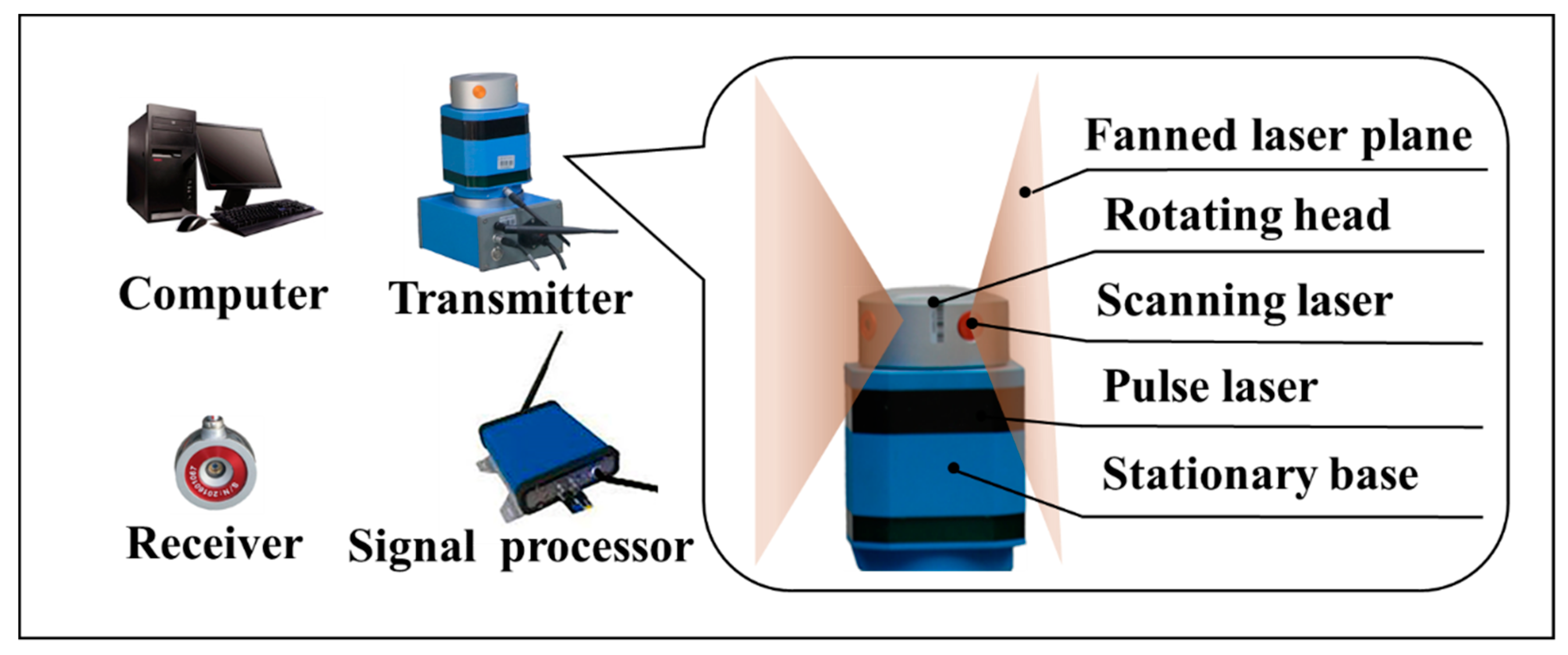
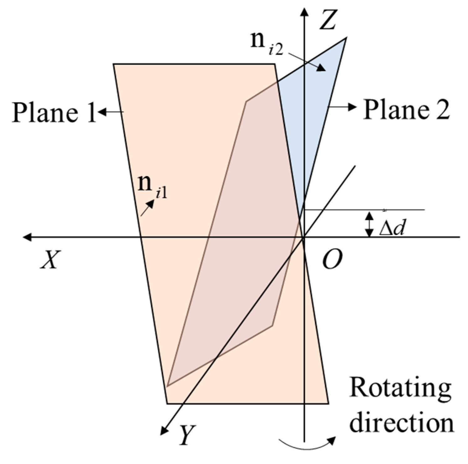
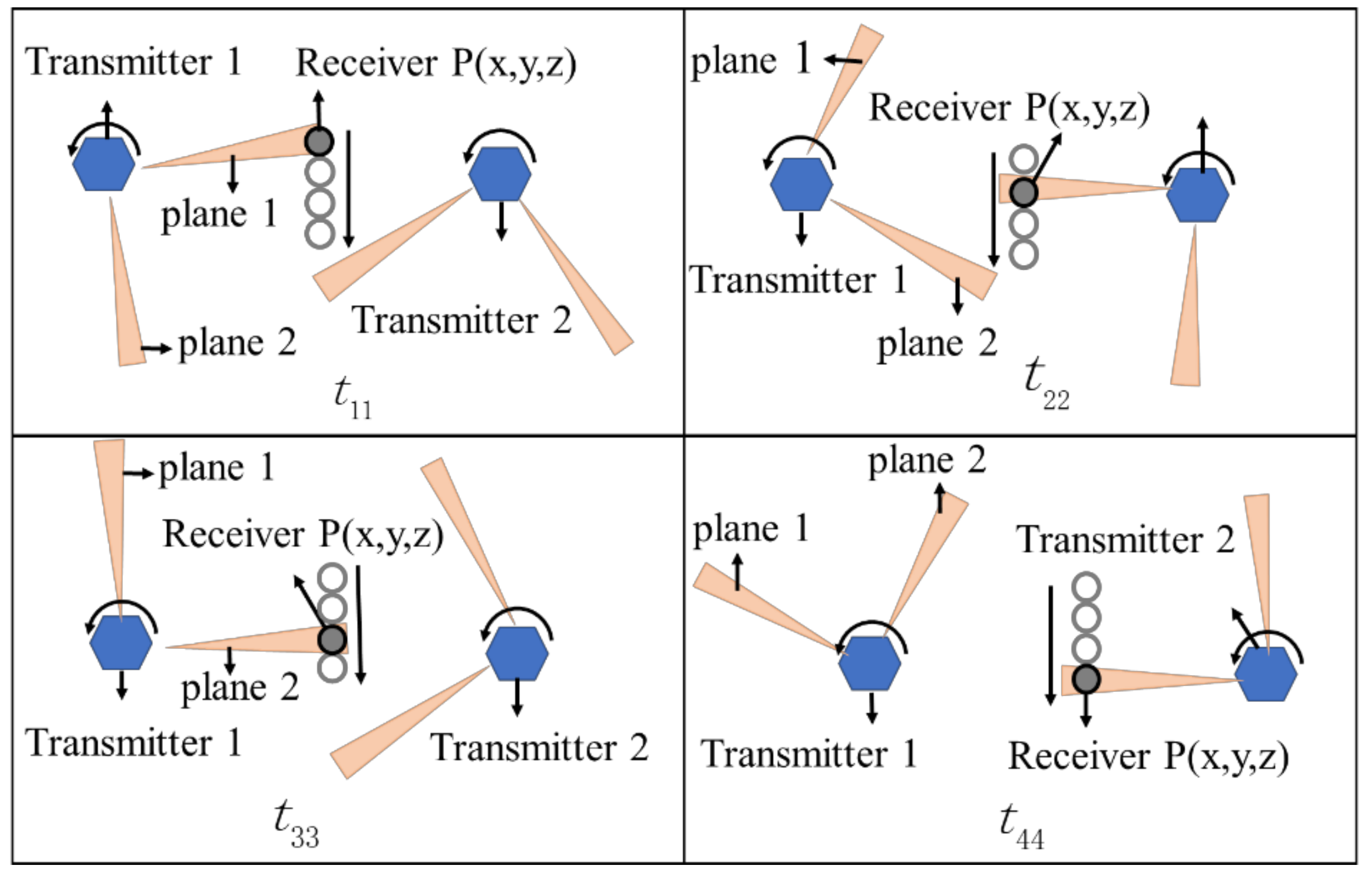
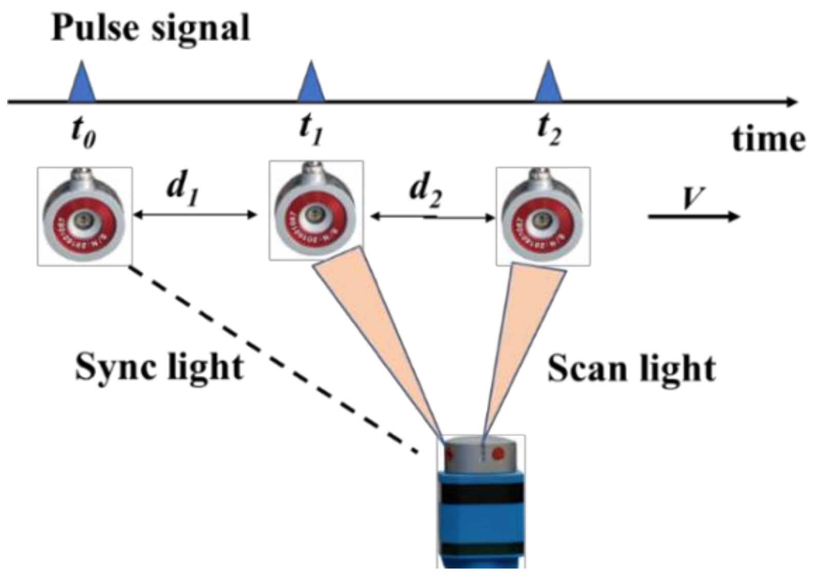
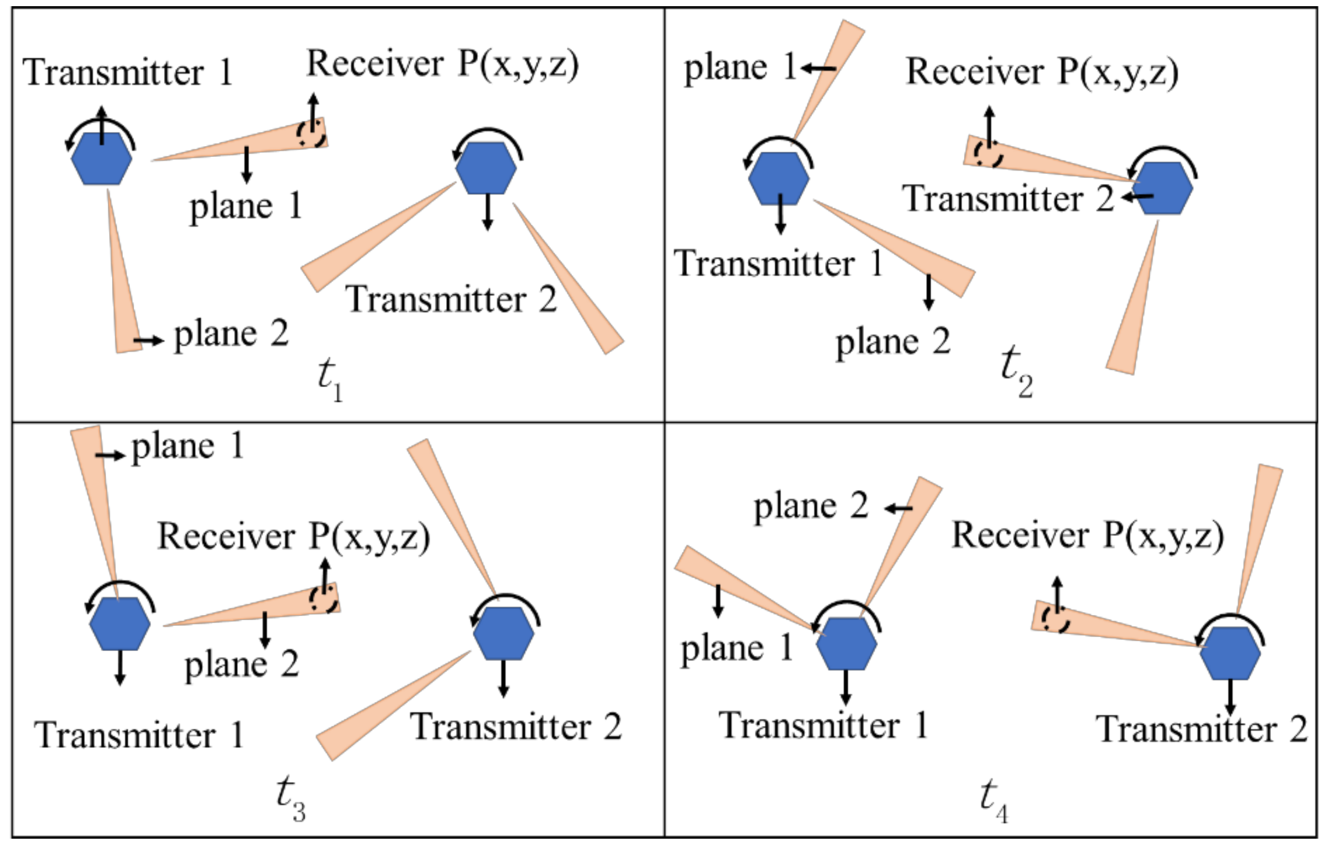
2. Basic Working Principle of wMPS
3. Test Description
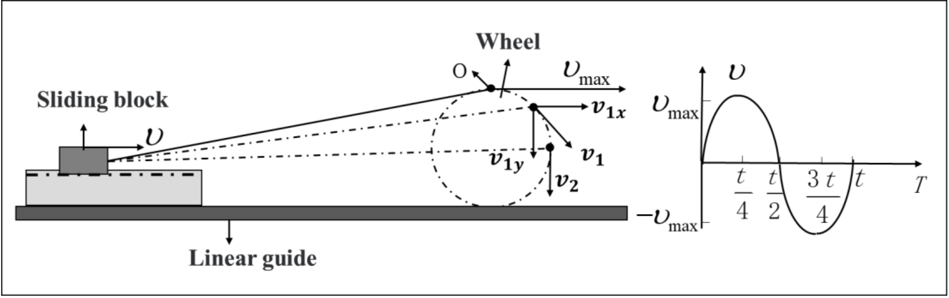
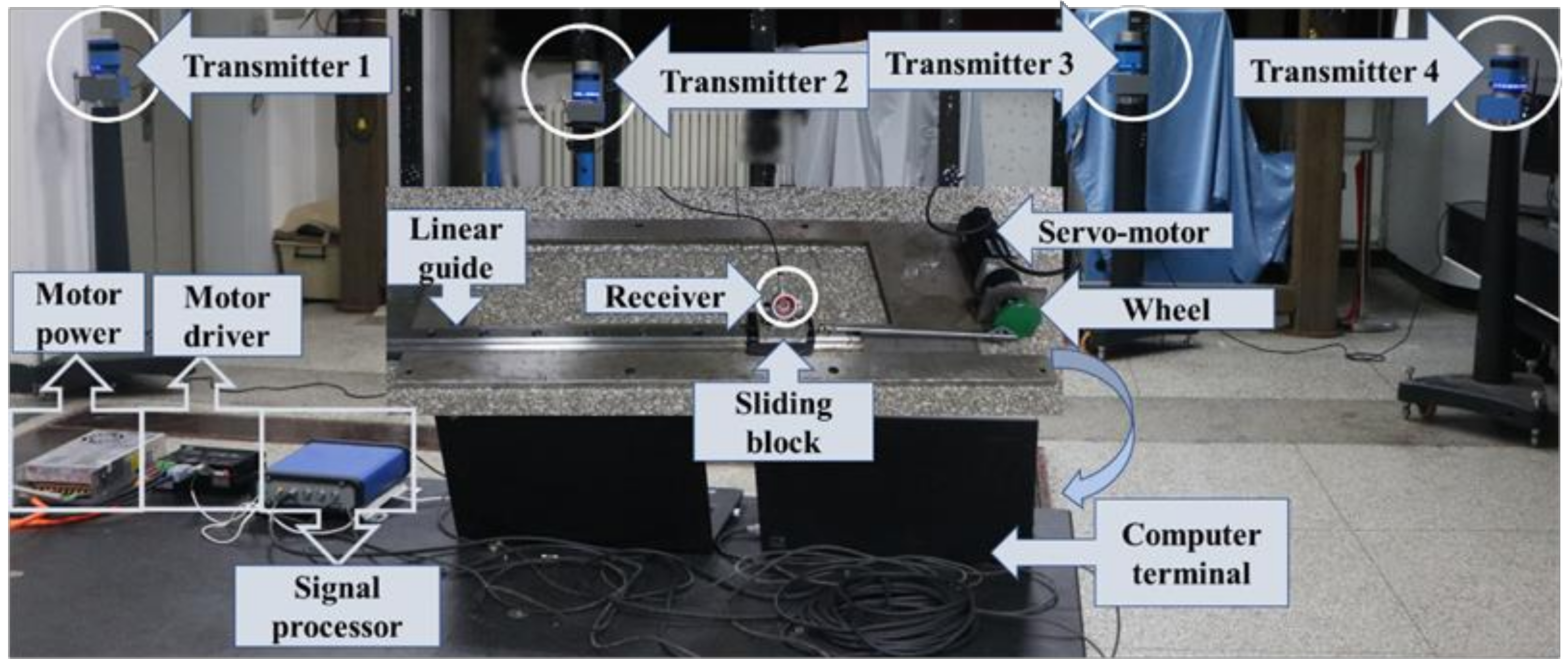
3.1. Test Equipment
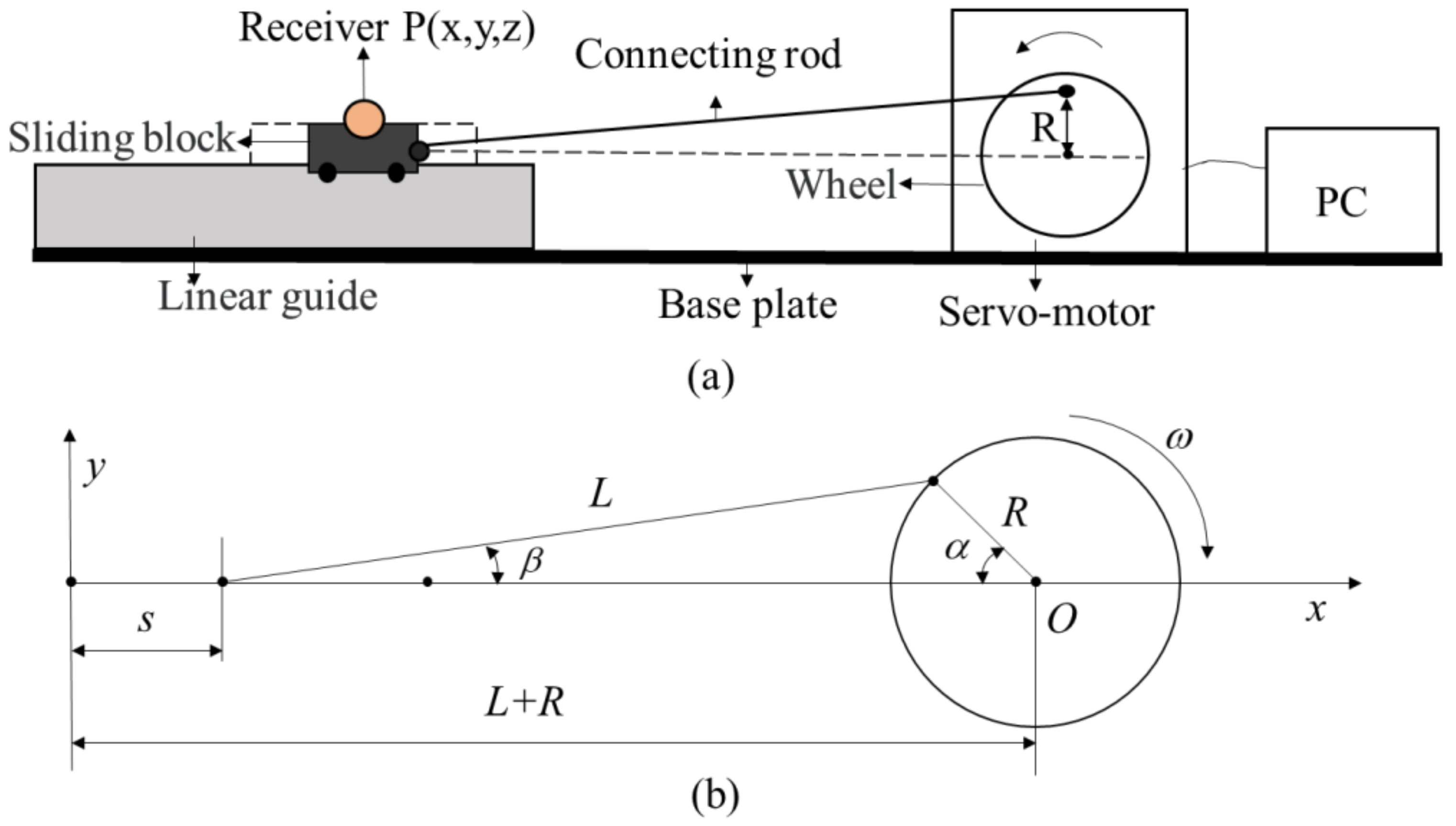
3.2. Test Method
4. Time-Series Analysis
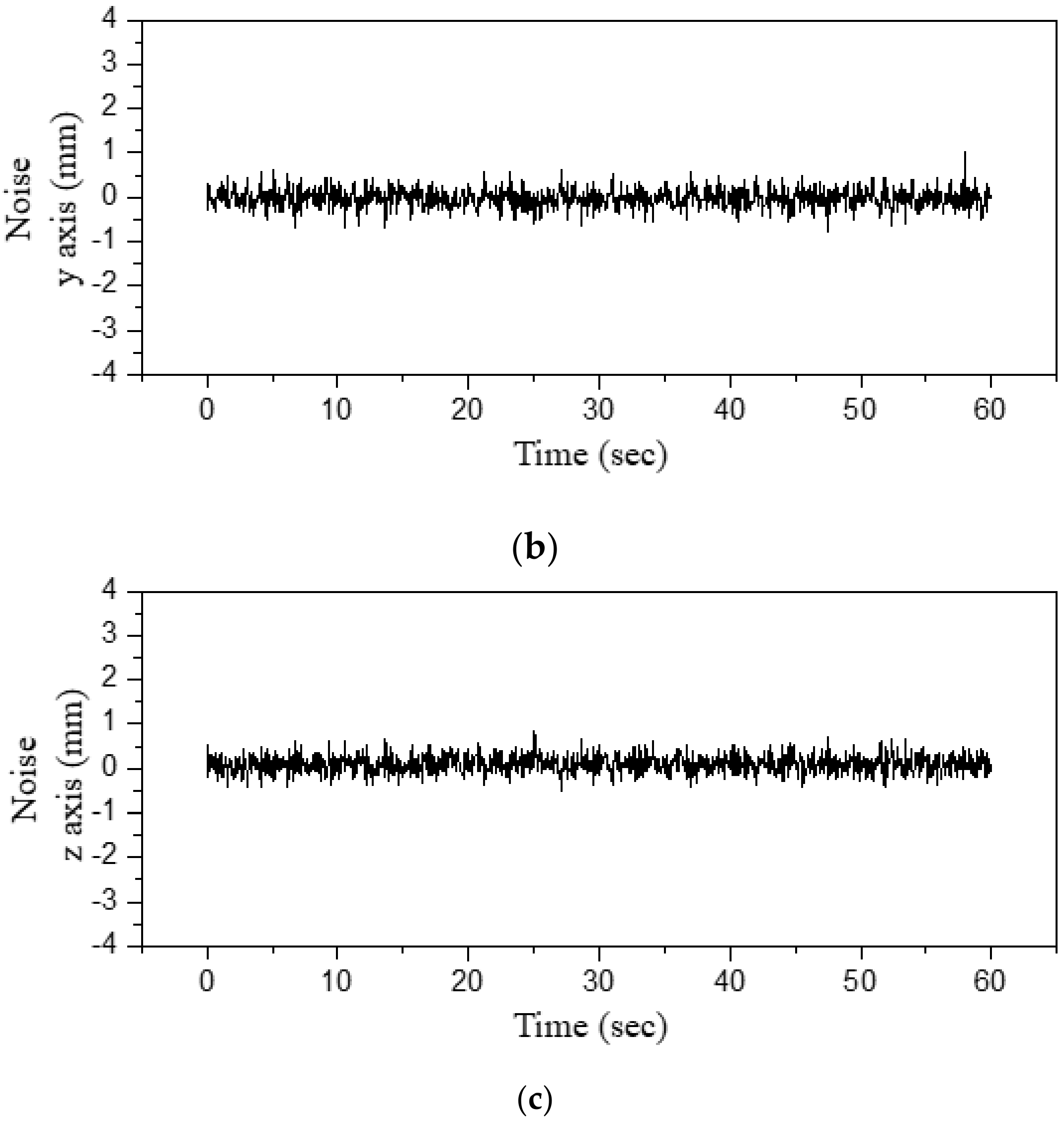
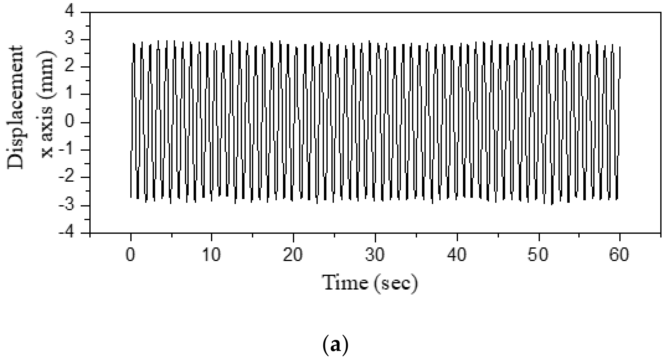
4.1. Data Preprocessing
4.2. Elimination of Gross Error
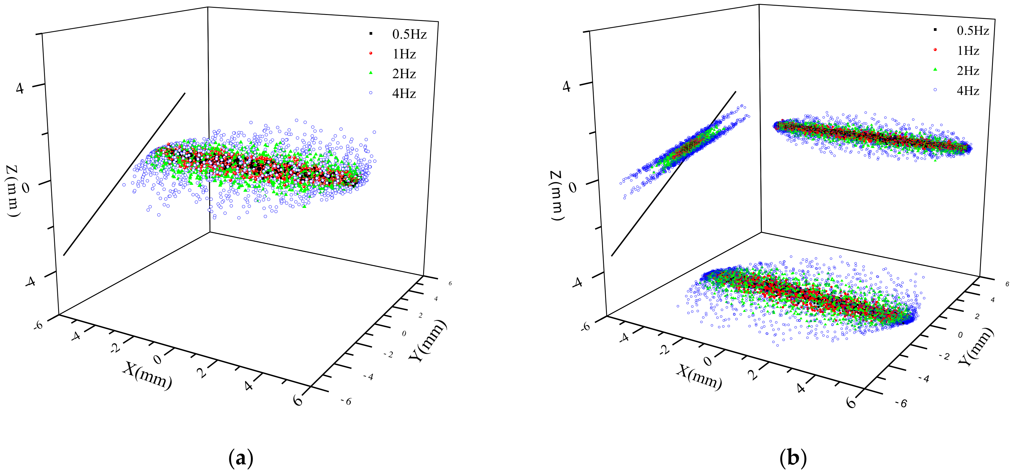
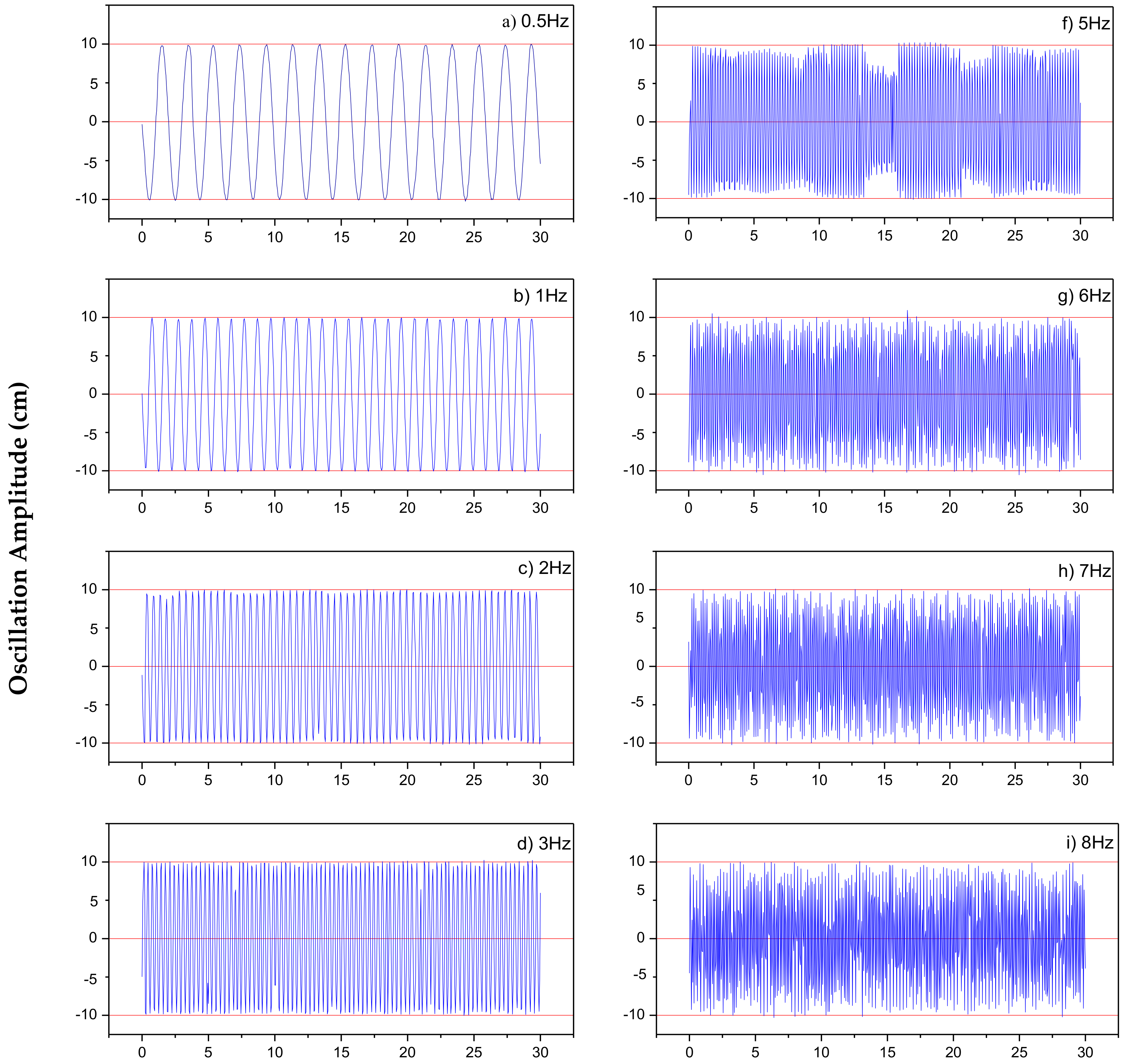
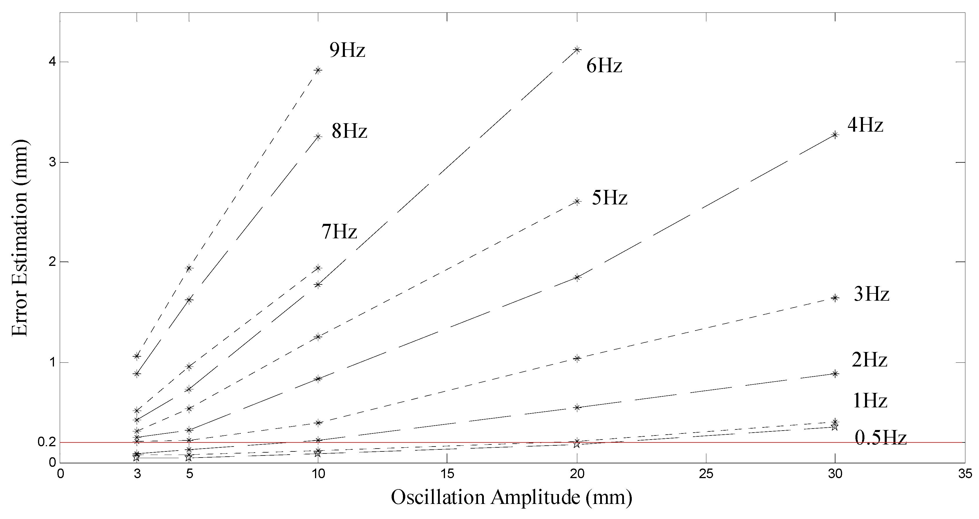
4.3. Assessment of the Potential of wMPS for Estimating the Oscillation Amplitude
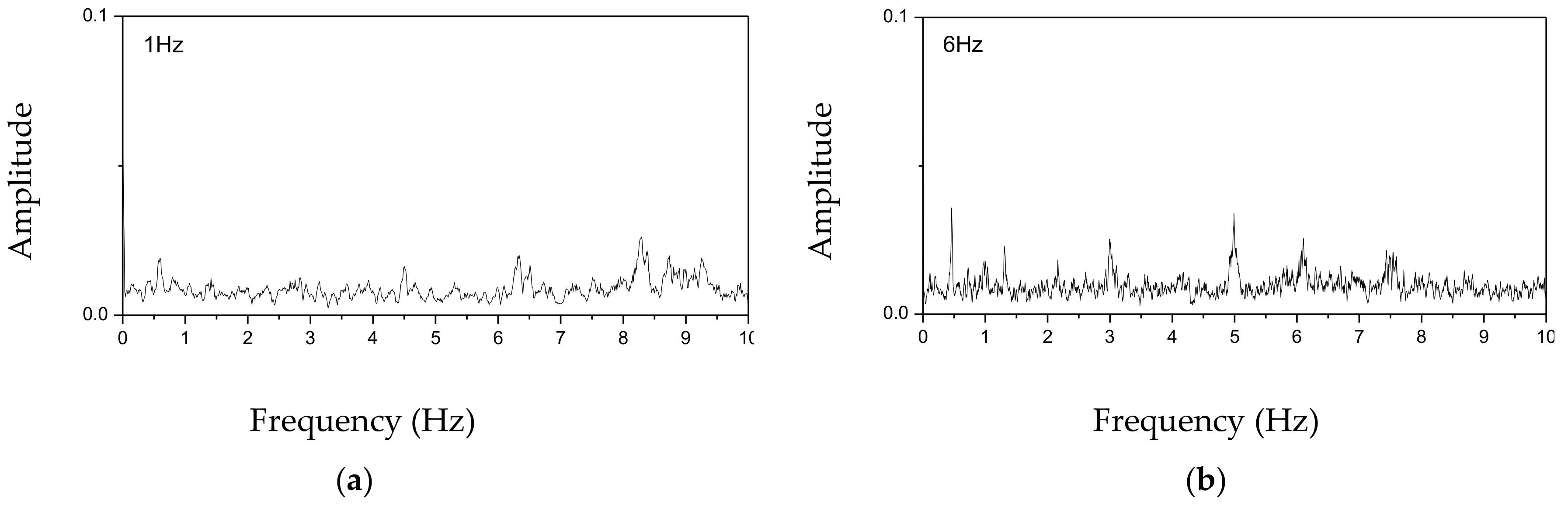
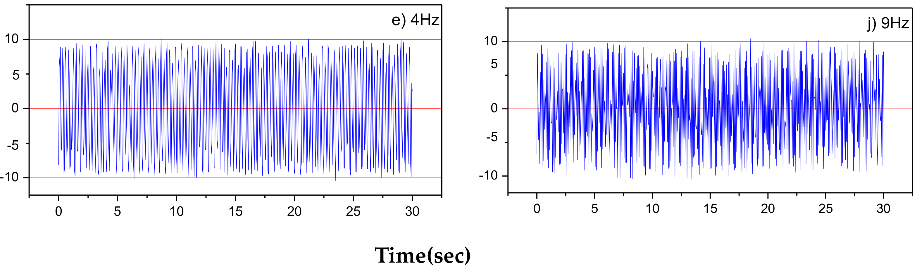
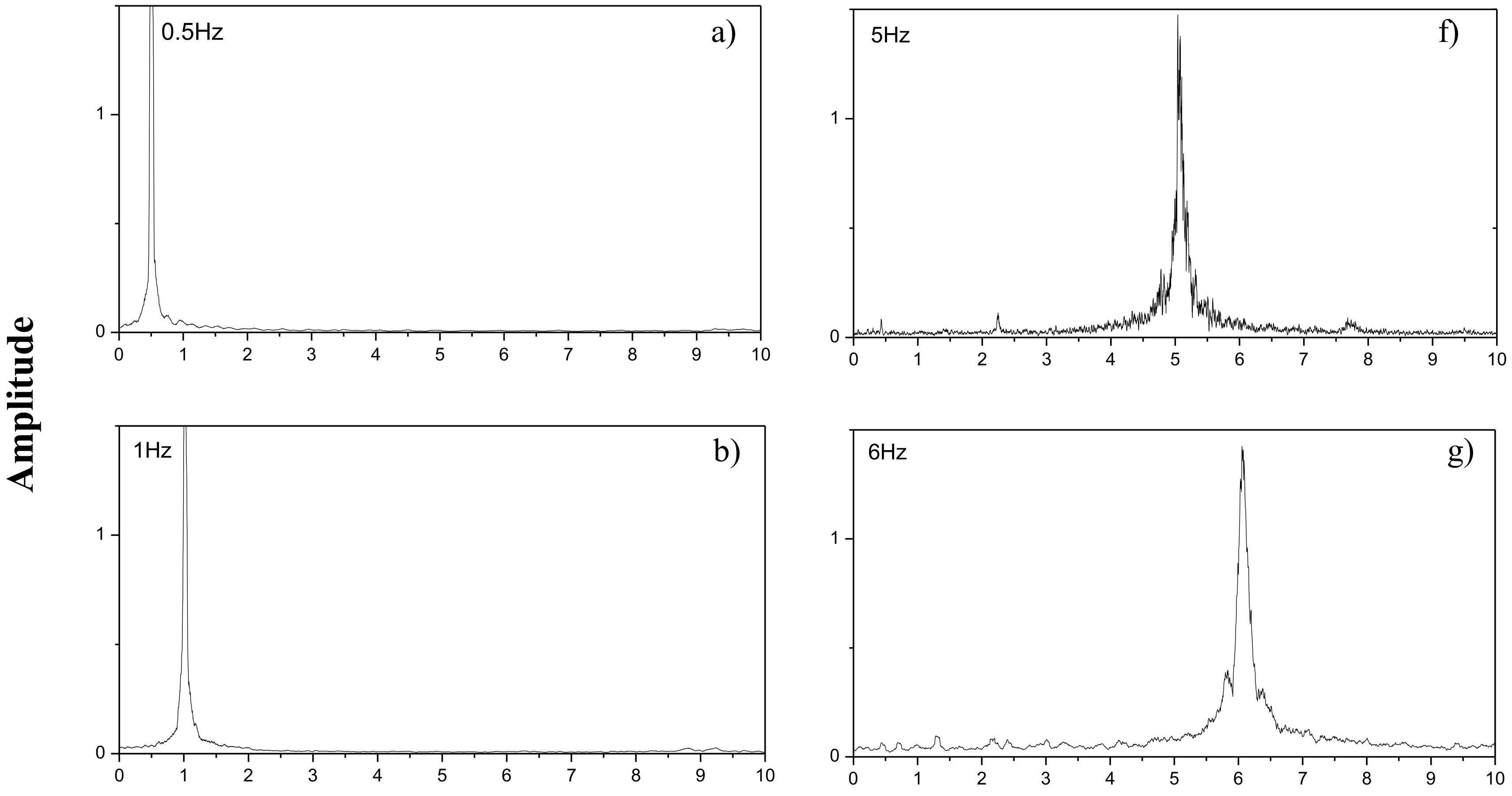
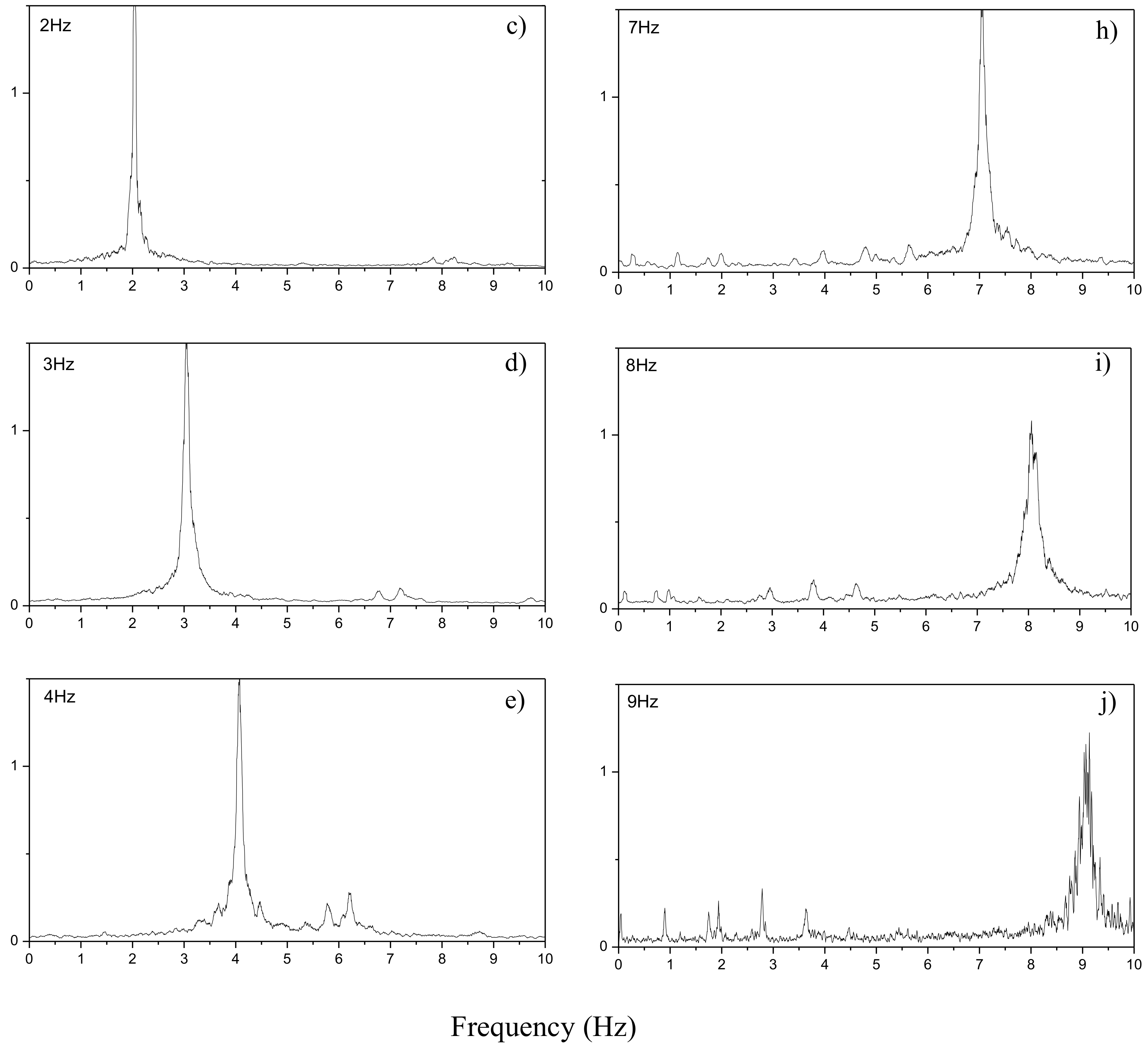
4.4. Extraction of Natural Frequency
5. Dynamic Error Analysis of the wMPS
6. Discussion
7. Conclusions
Author Contributions
Acknowledgments
Conflicts of Interest
Abbreviations
| GPS | global positioning system |
| RTS | robotic total station |
| wMPS | workspace measuring and positioning system |
| coordinate rotation matrices | |
| coordinate translation matrices | |
| β | swinging angle of connecting rod |
| deviation between the two planes along Z axis | |
| ni1 | normal vectors of plane 1 |
| ni2 | normal vectors of plane 2 |
| vmax | maximum slider speed |
| θj (j = 1,2) | rotation angle of the plane |
| R | crank throw |
| tj (j = 1,2) | record time |
| T | period |
| L | connecting rod length |
| λ | crank-link rod ratio |
| ω | angular velocity |
| s | slider displacement |
| f | frequency |
| v | slide speed |
| α | angle of rotation |
| R(θ) | plane rotation matrix |
References
- Glaser, S.D.; Li, H.; Wang, M.L.; Ou, J.; Lynch, J. Sensor technology innovation for the advancement of structural health monitoring: A strategic program of us-china research for the next decade. Smart Struct. Syst. 2007, 3, 221–244. [Google Scholar] [CrossRef]
- Jain, H.; Rawat, A.; Sachan, A.K. A review on advancement in sensor technology in structural health monitoring system. J. Struct. Eng. Manag. 2015, 2, 1–7. [Google Scholar]
- Şafak, E. Response of a 42-storey steel-frame building to the, ja:math, loma prieta earthquake. Eng. Struct. 1993, 15, 403–421. [Google Scholar] [CrossRef]
- Durukal, E. Dynamic response of two historical monuments in istanbul deduced from the recordings of kocaeli and duzce earthquakes. Bull. Seismol. Soc. Am. 2003, 93, 694–712. [Google Scholar] [CrossRef]
- Dong, D.; Fang, P.; Bock, Y.; Cheng, M.K.; Miyazaki, S. Anatomy of apparent seasonal variations from gps-derived site position time series. J. Geophys. Res. Solid Earth 2002, 107, ETG9-1–ETG9-16. [Google Scholar] [CrossRef]
- Breuer, P.; Chmielewski, T.; Górski, P.; Konopka, E. Application of gps technology to measurements of displacements of high-rise structures due to weak winds. J. Wind Eng. Ind. Aerodyn. 2002, 90, 223–230. [Google Scholar] [CrossRef]
- Nakamura, S.I. GPS measurement of wind-induced suspension bridge girder displacements. J. Struct. Eng. 2000, 126, 1413–1419. [Google Scholar] [CrossRef]
- Stiros, S.C. Errors in velocities and displacements deduced from accelerographs: An approach based on the theory of error propagation. Soil Dyn. Earthq. Eng. 2008, 28, 415–420. [Google Scholar] [CrossRef]
- Li, X.; Ge, L.; Ambikairajah, E.; Rizos, C.; Tamura, Y.; Yoshida, A. Full-scale structural monitoring using an integrated GPS and accelerometer system. GPS Solut. 2006, 10, 233–247. [Google Scholar] [CrossRef]
- Lovse, J.W.; Teskey, W.F.; Lachapelle, G.; Cannon, M.E. Dynamic deformation monitoring of tall structure using GPS technology. J. Surv. Eng. 1995, 121, 35–40. [Google Scholar] [CrossRef]
- Heo, G.; Kim, C.; Jeon, S.; Jeon, J. An Experimental Study of a Data Compression Technology-Based Intelligent Data Acquisition (IDAQ) System for Structural Health Monitoring of a Long-Span Bridge. Appl. Sci. 2018, 8, 361. [Google Scholar] [CrossRef]
- Yu, J.; Yan, B.; Meng, X.; Shao, X.; Ye, H. Measurement of bridge dynamic responses using network-based real-time kinematic GNSS technique. J. Surv. Eng. 2016, 142, 04015013. [Google Scholar] [CrossRef]
- Yan, Q.; Zhang, C.; Lin, G.; Wang, B. Field monitoring of deformations and internal forces of surrounding rocks and lining structures in the construction of the Gangkou double-arched tunnel—A case study. Appl. Sci. 2017, 7, 169. [Google Scholar] [CrossRef]
- Xu, L.; Guo, J.J.; Jiang, J.J. Time-frequency analysis of a suspension bridge based on GPS. J. Sound Vib. 2002, 254, 105–16. [Google Scholar] [CrossRef]
- Psimoulis, P.A.; Stiros, S.C. Measurement of deflections and of oscillation frequencies of engineering structures using Robotic Theodolites (RTS). Eng. Struct. 2007, 29, 3312–3324. [Google Scholar] [CrossRef]
- Psimoulis, P.; Pytharouli, S.; Karambalis, D.; Stiros, S. Potential of Global Positioning System (GPS) to measure frequencies of oscillations of engineering structures. J. Sound Vib. 2008, 318, 606–623. [Google Scholar] [CrossRef]
- Górski, P. Investigation of dynamic characteristics of tall industrial chimney based on GPS measurements using Random Decrement Method. Eng. Struct. 2015, 83, 30–49. [Google Scholar] [CrossRef]
- Chan, W.S.; Xu, Y.L.; Ding, X.L.; Xiong, Y.L.; Dai, W.J. Assessment of dynamic measurement accuracy of GPS in three directions. J. Surv. Eng 2006, 132, 108–117. [Google Scholar] [CrossRef]
- Psimoulis, P.A.; Stiros, S.C. Experimental assessment of the accuracy of GPS and RTS for the determination of the parameters of oscillation of major structures. Comput.-Aided. Civ. Inf 2008, 23, 389–403. [Google Scholar] [CrossRef]
- Moschas, F.; Stiros, S. PLL bandwidth and noise in 100 Hz GPS measurements. GPS Solut. 2015, 19, 173–185. [Google Scholar] [CrossRef]
- Schaal, R.E.; Larocca, A. Measuring dynamic oscillations of a small span cable-stayed footbridge: Case study using L1 GPS receivers. J. Surv. Eng. 2009, 135, 33–37. [Google Scholar] [CrossRef]
- Moschas, F.; Stiros, S. Measurement of the dynamic displacements and of the modal frequencies of a short-span pedestrian bridge using GPS and an accelerometer. Eng. Struct. 2011, 33, 10–17. [Google Scholar] [CrossRef]
- Moschas, F.; Stiros, S.C. Three-dimensional dynamic deflections and natural frequencies of a stiff footbridge based on measurements of collocated sensors. Struct. Control Health 2014, 21, 23–42. [Google Scholar] [CrossRef]
- Moschas, F.; Stiros, S. Dynamic deflections of a stiff footbridge using 100-Hz GNSS and accelerometer data. J. Surv. Eng. 2015, 141, 04015003. [Google Scholar] [CrossRef]
- Stiros, S.C.; Psimoulis, P.A. Response of a historical short-span railway bridge to passing trains: 3-D deflections and dominant frequencies derived from Robotic Total Station (RTS) measurements. Eng. Struct. 2012, 45, 362–371. [Google Scholar] [CrossRef]
- Stiros, S.; Moschas, F. Rapid decay of a timber footbridge and changes in its modal frequencies derived from multiannual lateral deflection measurements. J. Bridge Eng. 2014, 19, 05014005. [Google Scholar] [CrossRef]
- Yang, L.H.; Yang, X.Y.; Zhu, J.G.; Duan, M.; Lao, D. Novel method for spatial angle measurement based on rotating planar laser beams. Chin. J. Mech. Eng. 2010, 23, 758–764. [Google Scholar] [CrossRef]
- Norman, A.R.; Schönberg, A.; Gorlach, I.A.; Schmitt, R. Validation of iGPS as an external measurement system for cooperative robot positioning. Int. J. Adv. Manuf. Technol. 2013, 64, 427–446. [Google Scholar] [CrossRef]
- Lao, D.B.; Yang, X.Y.; Zhu, J.G.; Ye, S.H. Optimization of calibration method for scanning planar laser coordinate measurement system. Opt. Precis. Eng. 2011, 19, 870–877. [Google Scholar]
- Xiong, Z.; Zhu, J.G.; Zhao, Z.Y.; Yang, X.Y.; Ye, S.H. Workspace measuring and positioning system based on rotating laser planes. Mechanics 2012, 18, 94–98. [Google Scholar] [CrossRef]
- Zhao, Z.; Zhu, J.; Xue, B.; Yang, L. Optimization for calibration of large-scale optical measurement positioning system by using spherical constraint. J. Opt. Soc. Am. A 2014, 31, 1427–1435. [Google Scholar] [CrossRef] [PubMed]
- Guo, S.; Lin, J.; Ren, Y.; Shi, S.; Zhu, J. Application of a self-compensation mechanism to a rotary-laser scanning measurement system. Meas. Sci. Technol. 2017, 28, 115007. [Google Scholar] [CrossRef]
- Liu, Z.; Zhu, J.; Yang, L.; Liu, H.; Wu, J.; Xue, B. A single-station multi-tasking 3D coordinate measurement method for large-scale metrology based on rotary-laser scanning. Meas. Sci. Technol. 2013, 24, 105004. [Google Scholar] [CrossRef]
- Zhao, Z.; Zhu, J.; Lin, J.; Yang, L.; Xue, B.; Xiong, Z. Transmitter parameter calibration of the workspace measurement and positioning system by using precise three-dimensional coordinate control network. Opt. Eng. 2014, 53, 084108. [Google Scholar] [CrossRef]
- Yang, L.H.; Zhu, J.G.; Zhang, G.J.; Ye, S.H. Orientation method for workspace measurement positioning system based on scale bar. J. Tianjin Univ. 2012, 45, 814–819. [Google Scholar]


| Frequency (Hz) | Amplitude (mm) | ||||
|---|---|---|---|---|---|
| 3 | 5 | 10 | 20 | 30 | |
| 0.5 | 0.05 ± 0.06 | 0.05 ± 0.06 | 0.09 ± 0.11 | 0.18 ± 0.19 | 0.35 ± 0.36 |
| 1 | 0.08 ± 0.09 | 0.08 ± 0.09 | 0.12 ± 0.17 | 0.21 ± 0.25 | 0.41 ± 0.44 |
| 2 | 0.09 ± 0.11 | 0.13 ± 0.17 | 0.22 ± 0.31 | 0.55 ± 0.71 | 0.89 ± 1.27 |
| 3 | 0.21 ± 0.23 | 0.22 ± 0.33 | 0.39 ± 0.60 | 1.04 ± 1.43 | 1.65 ± 2.19 |
| 4 | 0.25 ± 0.37 | 0.32 ± 0.46 | 0.84 ± 1.11 | 1.85 ± 2.65 | 3.28 ± 4.40 |
| 5 | 0.31 ± 0.44 | 0.54 ± 0.78 | 1.26 ± 1.83 | 2.61 ± 3.38 | - |
| 6 | 0.43 ± 0.64 | 0.73 ± 1.09 | 1.45 ± 2.14 | 4.13 ± 6.01 | - |
| 7 | 0.52 ± 0.69 | 0.96 ± 1.23 | 1.94 ± 2.44 | - | - |
| 8 | 0.89 ± 1.16 | 1.62 ± 2.05 | 3.25 ± 4.08 | - | - |
| 9 | 1.06 ± 1.35 | 1.94 ± 2.39 | 3.92 ± 4.80 | - | - |
| Frequency (Hz) | Amplitude (mm) | ||||
|---|---|---|---|---|---|
| 3 | 5 | 10 | 20 | 30 | |
| 0.5 | 0.506 | 0.506 | 0.504 | 0.506 | 0.511 |
| 1 | 1.010 | 1.007 | 1.025 | 1.019 | 1.014 |
| 2 | 2.039 | 2.038 | 2.040 | 2.051 | 2.048 |
| 3 | 3.054 | 3.053 | 3.076 | 3.003 | 3.081 |
| 4 | 4.081 | 4.087 | 4.049 | 4.069 | 4.155 |
| 5 | 5.086 | 5.059 | 5.076 | 5.123 | - |
| 6 | 6.066 | 6.036 | 6.040 | 6.102 | - |
| 7 | 7.095 | 7.036 | 7.033 | - | - |
| 8 | 8.123 | 8.086 | 8.035 | - | - |
| 9 | 9.110 | 9.100 | 9.132 | - | - |
© 2019 by the authors. Licensee MDPI, Basel, Switzerland. This article is an open access article distributed under the terms and conditions of the Creative Commons Attribution (CC BY) license (http://creativecommons.org/licenses/by/4.0/).
Share and Cite
Xiong, C.; Bai, H.; Lin, J. Potential of Workshop Measurement Positioning System to Measure Oscillation Frequencies of Rigid Structures. Appl. Sci. 2019, 9, 595. https://doi.org/10.3390/app9030595
Xiong C, Bai H, Lin J. Potential of Workshop Measurement Positioning System to Measure Oscillation Frequencies of Rigid Structures. Applied Sciences. 2019; 9(3):595. https://doi.org/10.3390/app9030595
Chicago/Turabian StyleXiong, Chunbao, Hongzhi Bai, and Jiarui Lin. 2019. "Potential of Workshop Measurement Positioning System to Measure Oscillation Frequencies of Rigid Structures" Applied Sciences 9, no. 3: 595. https://doi.org/10.3390/app9030595
APA StyleXiong, C., Bai, H., & Lin, J. (2019). Potential of Workshop Measurement Positioning System to Measure Oscillation Frequencies of Rigid Structures. Applied Sciences, 9(3), 595. https://doi.org/10.3390/app9030595