Detection of Helminthosporium Leaf Blotch Disease Based on UAV Imagery

Abstract

Helminthosporium leaf blotch (HLB) is a serious disease of wheat causing yield reduction globally. Usually, HLB disease is controlled by uniform chemical spraying, which is adopted by most farmers. However, increased use of chemical controls have caused agronomic and environmental problems. To solve these problems, an accurate spraying system must be applied. In this case, the disease detection over the whole field can provide decision support information for the spraying machines. The objective of this paper is to evaluate the potential of unmanned aerial vehicle (UAV) remote sensing for HLB detection. In this work, the UAV imagery acquisition and ground investigation were conducted in Central China on April 22th, 2017. Four disease categories (normal, light, medium, and heavy) were established based on different severity degrees. A convolutional neural network (CNN) was proposed for HLB disease classification. The experiments on data preprocessing, classification, and hyper-parameters tuning were conducted. The overall accuracy and standard error of the CNN method was 91.43% and 0.83%, which outperformed other methods in terms of accuracy and stabilization. Especially for the detection of the diseased samples, the CNN method significantly outperformed others. Experimental results showed that the HLB infected areas and healthy areas can be precisely discriminated based on UAV remote sensing data, indicating that UAV remote sensing can be proposed as an efficient tool for HLB disease detection.

1. Introduction

Helminthosporium leaf blotch (HLB) is a serious disease of wheat cultivation, which causes yield reduction globally [1]. Yield losses due to HLB were reported, and the reduction up to 20% were observed in [2,3]. Usually, the HLB disease is controlled by uniform spraying of chemicals. However, increased use of chemicals has caused agronomical and environmental problems [4]. To solve this problem, accurate chemical spraying could be a key solution [5]. Accurate spraying emphasizes applying adequate doses of chemicals based on the degree of disease infection [6]. Thus, it is possible to reduce the use of chemicals. On the other hand, accurate spraying applies enough chemicals according to the specific requirement of disease degrees, which may enhance the chemical effects. In this case, effective detection of the disease could provide detailed support information for the spraying machines. Traditional assessment of the HLB disease is made by manual investigation throughout the field, which is laborious and time-consuming [7].

Remote sensing (RS) has been frequently used as an effective, efficient, and safe tool for rapid detection of plant diseases [8,9,10,11]. Compared with satellite and aircraft remote sensing, unmanned aerial vehicle (UAV) can fly at a low altitude and capture high resolution imagery [12], which would provide more detailed spatial information for plant disease detection. There are literatures applying UAV remote sensing for detection of wheat diseases. Feng et al. [13] applied the UAV remote sensing for monitoring wheat stripe rust. Correlation analysis between the disease index and the image reflectance were conducted. The linear regression method was used to build the estimation model. A significant difference between the reflectance of the healthy plots and diseased plots was observed, which indicated that UAV-based monitoring of wheat stripe rust was feasible. Liu et al. [14] employed the UAV imagery to detect the wheat powdery mildew. UAV imagery were captured at different altitudes over the wheat fields. Fitting the data with random coefficient regression models, the exact relationship between the image parameter lgR and the disease severity was observed. However, to our best knowledge, the research on HLB disease detection using UAV imagery cannot be accessed yet. The objective of this paper was to evaluate the potential of UAV-based imagery for HLB disease detection. In the framework of this research, it is unfeasible to distinguish other pathologies that may also cause similar symptoms as HLB disease. However, it is the first step to detect the disease infection, which may build a significant foundation for further analysis.

The rest of this paper is organized as followed: Section 2 introduces the data collection and the processing methods; Section 3 demonstrates the experimental results of our methods and the comparison with other methods, and Section 4 describes the conclusion and further perspective.

2. Materials and Methods

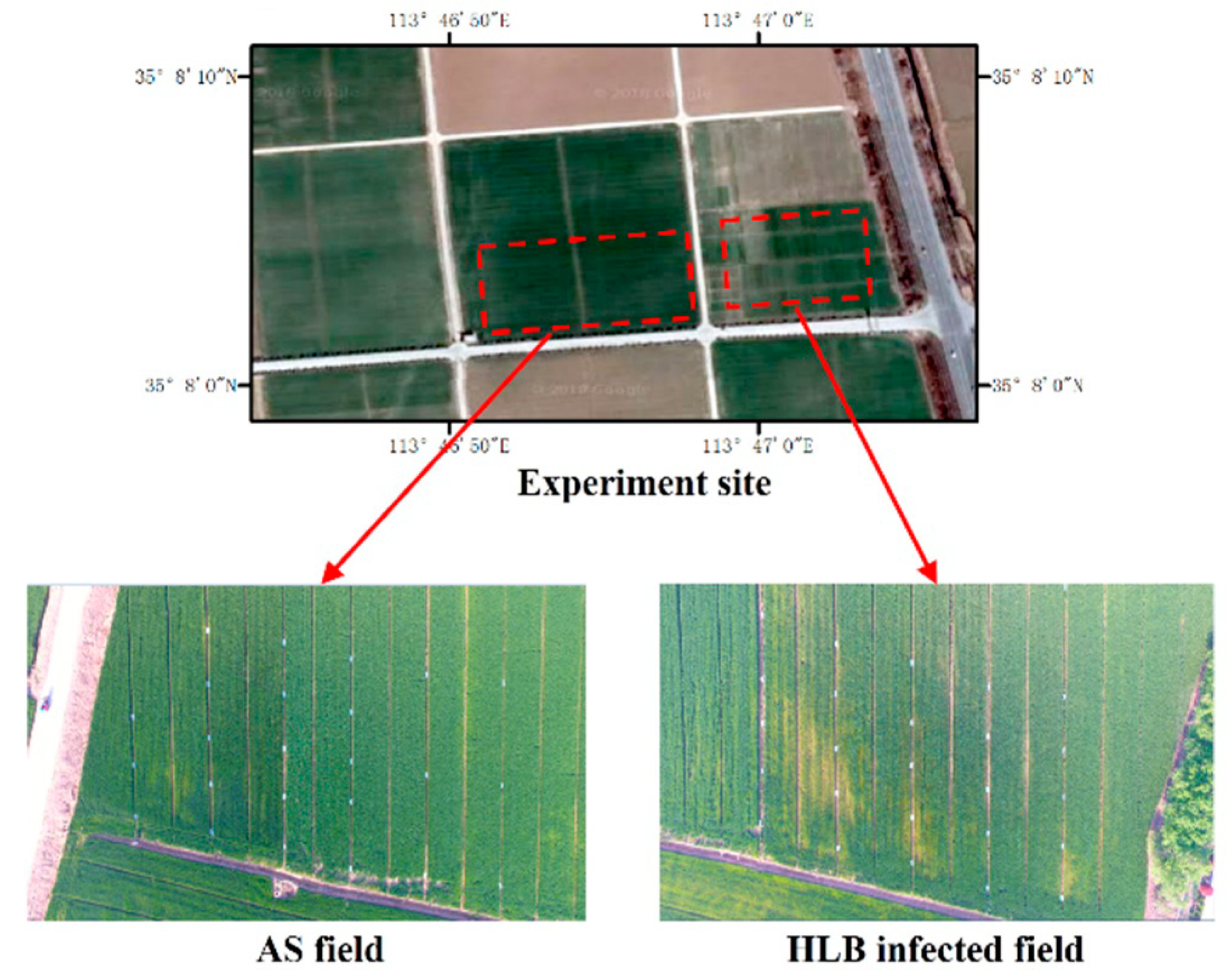
2.1. Study Site

The study site was located in Xinxiang city, Henan province, China (35°8′4 N, 113°46′56 E). Wheat was planted within this field, with a row spacing of 1 meter. Two fields were selected for the experiment. One is infected with HLB, and the other is asymptomatic (AS), as shown in Figure 1. UAV flights and field campaigns were conducted under cloud-free conditions on April 22nd, 2017, when the wheat was in its heading period. The HLB infection was in its initial stage when most of the infected leaves started to turn yellow.

2.2. Data Collection

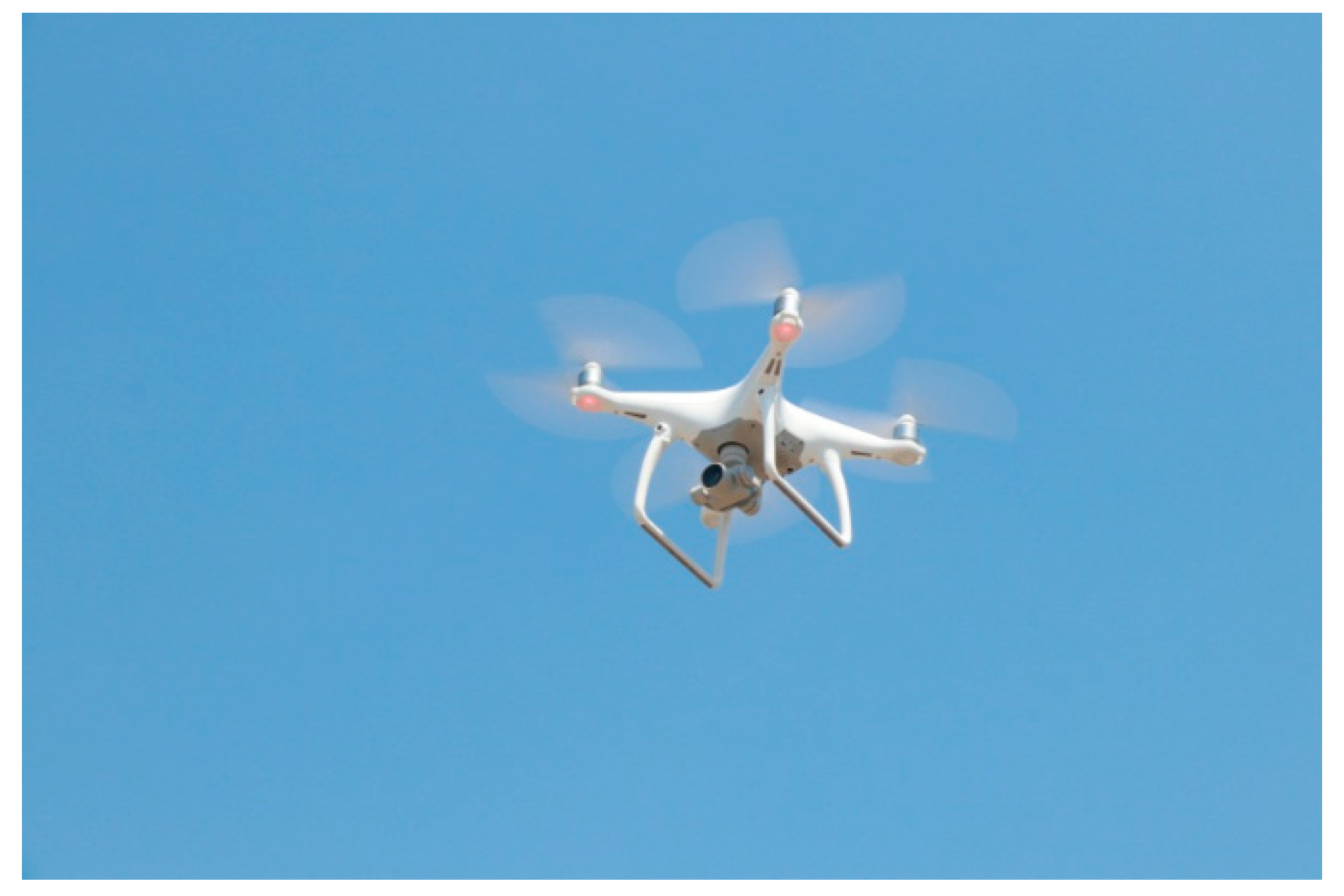
2.2.1. UAV Imagery Collection

A multi-rotor UAV, Phantom 4 (DJI Co., Shenzhen, China) was used for data collection, as shown in Figure 2. Phantom 4 is able to fly autonomously or by a remote controller with an integration of a GPS receiver. The technical characteristics of the UAV information are presented in

Table 1. Technical characteristics of Phantom 4 and its onboard camera.

Phantom 4	Quad-Rotor UAV
Cross weight	1380 g
Diagonal Size	350 mm
Max Speed	20 m/s
Max Flight Time	28 minutes
Size	4000 × 300 pixels
Lens	FOV 94°20 mm
Typical spatial resolution (at 80 m altitude)	3.4 cm/pixel

. Its onboard camera is a standard Red-Green-Blue (RGB) camera, and the captured imagery is 4000 × 3000 pixels in size. The UAV imagery of the HLB and the AS fields was collected at the height of 80 m, with the spatial resolution of 3.4 cm.

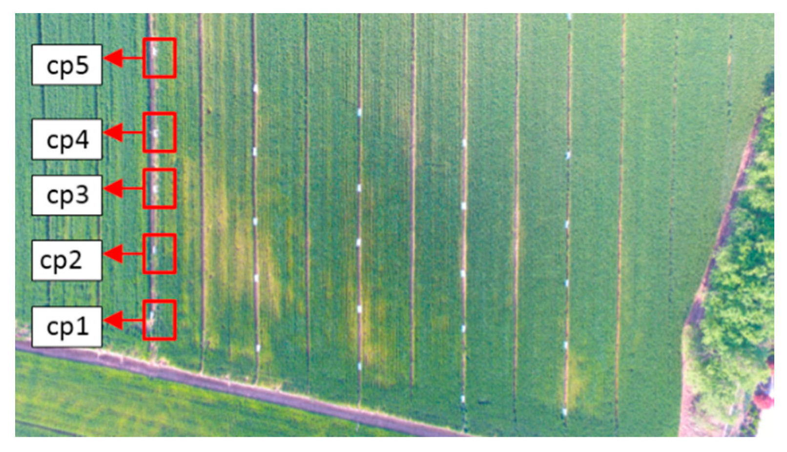
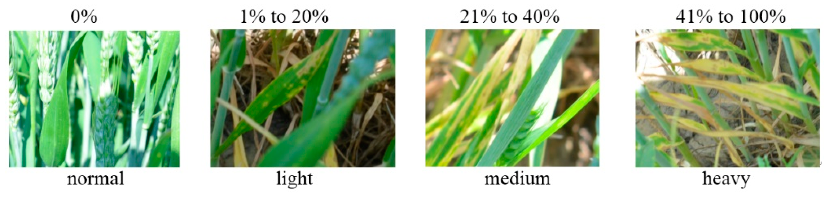
2.2.2. Ground Investigation

Ground investigation consisted of recording the disease severity and precise location of all the sites presenting symptoms. Following the location strategy of [15], ground control point markers (0.9 m × 0.4 m white board) were placed in the field, where each marker was assigned with a specific number (cp1, cp2, etc.) to represent the accurate location of an investigation site, as illustrated in Figure 3. In each site presenting HLB symptoms, the disease severity degree and ground control point number were recorded.

According to [9], plant disease severity corresponds to the percentage of the sample units showing visual symptoms of disease. The HLB disease severities were classified into four categories (normal, light, medium, heavy), as illustrated in Figure 4.

2.3. Data Analysis

Convolutional neural networks (CNN) are an example of specialized neural network architecture, which has been proven a successful method in many vision classification applications [16]. In this work, CNN was adopted for HLB disease classification. Our CNN framework shared the basic architecture of the classic LeNet-5 [16], while some adjustments were carried out to fit our data. This network architecture is composed of three modules: (1) Preprocessing; (2) Feature extraction; (3) Classification, as shown in Figure 5.

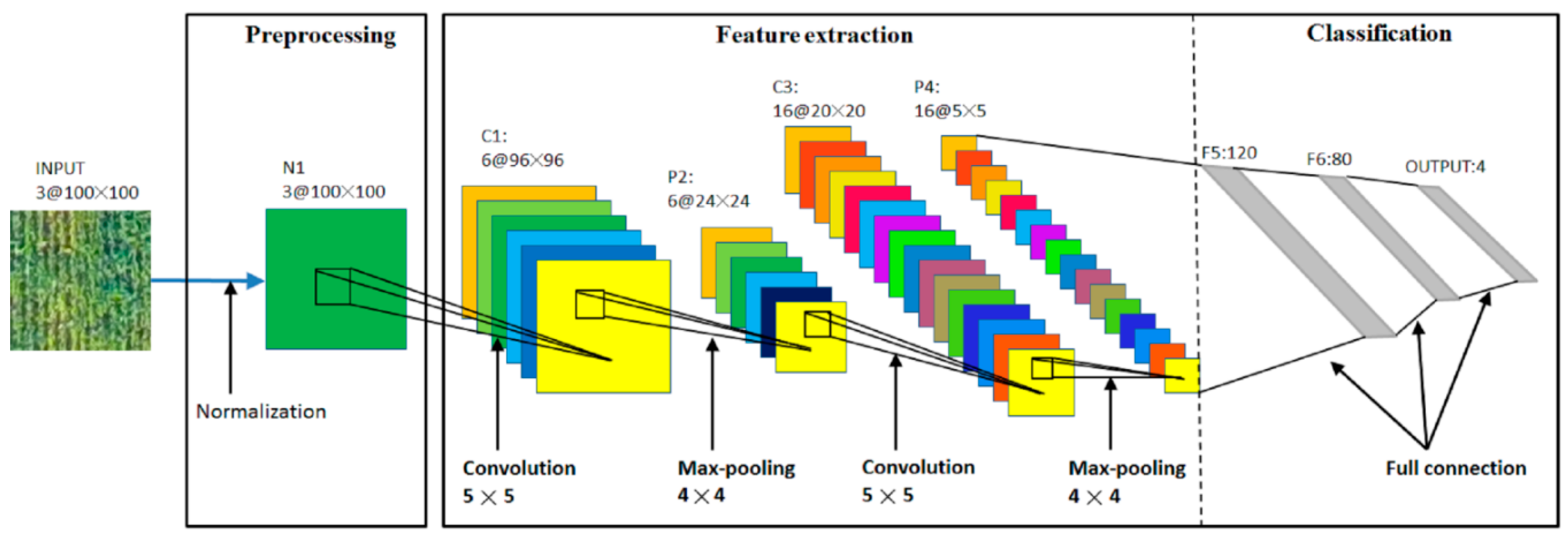
2.3.1. Preprocessing

Before feature extraction and classification, a batch normalization operation was performed for each input image to solve the problem of internal covariate shift. The application of batch normalization generally stabilizes the training process, even with a higher learning rate [17]. In our CNN architecture, preprocessing is a normalization step that fixes the mean and variances of input image.

2.3.2. Feature Extraction

Finding good image features could significantly build a good foundation for the next step of classification [18]. The feature extraction strategy has a strong effect on the final performance of the classifier [19]. Unlike traditional feature extraction, CNN is capable of automatically extracting effective features and overcoming the over fitting problem. This architecture strongly improves the performance of remote sensing imagery classification [7], object detection [20], and segmentation [21].

The feature extraction module in CNN architecture is a cascade of multiple stages. The input and output of each stage are sets of arrays called feature maps [22]. In each stage, the output represents a feature map extracted at all locations on input. In general, each stage is composed of two layers: convolutional and pooling.

The convolutional layer is the core building block for CNN that contains a set of learnable filters. With the trainable weights in each filters, updated with the training losses during backpropagation, the output of the convolutional layer effectively learns particular features of input arrays. Let x denote the input array with l_x feature maps, y denotes the output array with l_y feature maps, W_ij denotes a two-dimensional weight that associates the ith feature map in the input and the jth feature map in the output. The equation between x and y is denoted in (1), where * is the 2D discrete convolution operator and b_j is a trainable bias parameter.

$${\mathrm{y}}_j={{\displaystyle \sum }}_{i=1}^{l_x}{W}_{ij}\ast x_i+b_j(j=1,2,\dots ,l_y)$$

(1)

After convolution, a non-linear activation function, which can be sigmoid, tanh or rectified linear function (ReLu) [23] applied in an element-wise manner. Although there are many types of activation functions, ReLu is widely used in CNN algorithm. ReLus are easy to implement and meaningful for accelerating the convergence of the training process [19].

Pooling operator computes the average value or selects the maximum value over a neibourhood on each feature map. This operator generates a smaller output feature map which is robust to some variations of the input feature map [22]. Max-pooling and average-pooling are the usual pooling types in CNN, while max-pooling generally performs better than average-pooling.

2.3.3. Classification

In this work, three fully connected layers were designed for the classification tasks. The first fully connected layer (the sixth layer, denoted as F5 in Figure 5) takes the cascade of all feature maps of the fifth layer (denoted as h₅) as input. Let us denote that the weights and bias of this layer as W₆ and b₆, respectively. The output of this layer (denoted as h₆) can be denoted as (2):

$$h_6=\mathsf{\phi }\left(W_6{h}_5+b_6\right)$$

(2)

where the symbol $\mathsf{\phi }(·)$ denotes a non-linear activation function, W₆ and b₆ represent the connected weights and biases respectively. Similar with the convolutional operation, ReLu was employed as the activation function.

The last fully connected layer is the output layer, which exports the probabilities of different HLB disease categories. This layer has four neurons corresponding to four HLB disease categories (normal, light, medium, and heavy). Let us denote the output of this layer is y = [y₁ y₂ y₃ y₄], where y_i is the output probability for the ith category. Thus, the maximum value in y ([y₁ y₂ y₃ y₄]) corresponds to the final classified category.

2.4. Algorithms in Comparison

In Section 2.3, we exploited the strong power of CNN. After that, we compared its performance with some traditional classification approaches, which extracted hand craft features for the classifiers. In this section, three types of hand craft features were consider: color histogram, local binary pattern histogram, and vegetation index. The reasons for feature selection are that for: (1) the color histogram, the color difference of healthy and diseased wheat can be visually distinguished, which may result in the difference of the color histogram; (2) the LBP feature, the disease infection may cause texture variation in UAV imagery, and (3) the vegetation index, it has the potential to detect crop stress [9].

2.4.1. Color Histogram

Given a color space of an image, the color histogram is calculated by counting the times of each color occurs in the array of image data [24]. In this work, the color histograms of all channels (red, green, and blue) were calculated respectively and concatenated as the feature vector.

2.4.2. Local Binary Pattern Histogram

The original local binary pattern histogram (LBPH) was introduce by Ojala, T [25] for texture feature extraction. For each pixel in the image, the operator thresholds a 3 × 3 neighborhood with the center value and considers the comparison result as a binary number, which is the new value of that pixel [26]. Then the histogram of the label image could be considered as the texture feature descriptor. The LBPH method has been successfully used in image classification tasks, especially in face recognition [26]. In this work, LBPH was adopted to extract texture features for HLB disease category classification.

2.4.3. Vegetation Index

Eight vegetation indices (VI) were calculated as the feature vector of the UAV imagery. They were calculated because of their potential to discriminate different HLB infected categories. The UAV imagery only contained the RGB bands in this work. Thus, VI involved with other bands cannot be used. Instead, several VI only involved with RGB bands were selected.

Table 2. Summary of selected vegetation indices.

Index	Formula	References
Normalized Green–Red Difference Index	$NGRDI=\frac{Green-Red}{Green+Red}$	[27]
Normalized Green–Blue Difference Index	$NGBDI=\frac{Green-Blue}{Green+Blue}$	[28]
Excess Green	ExG = 2 × Green-Red-Blue	[29]
Excess Red	ExR = 1.4 × Red-Green	[30]
Excess Green - Excess Red	ExGR = 3×Green-2.4 × Red-Blue	[30]
Green Leaf Index	$GLI=\frac{2\times Green-Red-Blue}{2\times Green+Red+Blue}$	[31]
Red–Green Rate Index	RGRI = Red/Green	[32]
Blue–Green Rate Index	BGRI = Blue/Green	[32]

listed the formula and references of the selected vegetation indices.

2.4.4. Support Vector Machine

In support vector machine (SVM) solutions, a large margin strategy and kernel mapping technique are used for tasks of classification. In the past years, it has been proven that SVM solutions have outperformed many existing methods on several classification and nonlinear function estimation problems [33]. Especially in the small-size training dataset, SVM performs well with good generalization capability [34]. Since the training dataset size was small in this study, the SVM method was applied for classification based on the features extracted in Section 2.4.1, Section 2.4.2 and Section 2.4.3.

3. Results and Discussion

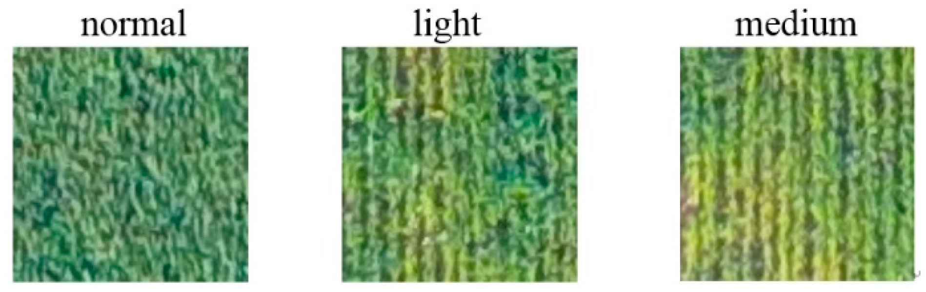
3.1. Dataset Preparation

The resolution of UAV imagery is 4000 × 3000. According to the result of the ground investigation, the symptomatic sites were mainly distributed in 3 × 3 m areas in different locations of the field. As shown in Table 1, the imagery was captured at a height of 80 m, with a resolution of 3.4 cm. To reflect the areas (3 m × 3 m) of the symptomatic sites, smaller samples were divided from the original UAV imagery in the size of 100 × 100 pixels. Two thousand and four hundred samples were generated from the collected imagery. Each sample represented a small area in the wheat field and was assigned a certain label (normal, light, medium, and heavy) according to the ground investigation results.

At this point, the dataset was composed of a collection of samples divided from the original UAV imagery. Each sample consisted of 100 × 100 pixels and a label (normal, light, medium, and heavy) according to the ground investigation. Since the experiment was conducted when HLB disease was in its initial stage, no heavy category was found in the field, as shown in Figure 6.

Next, the dataset was divided into two parts: (a) training samples; (b) validation samples. At this stage of the work, 60% of samples in each category were randomly selected as the training samples, while the remaining 40% as the validation samples. In our dataset, the number of normal samples was larger than other categories. To avoid the problem of data imbalance, similar numbers of each category were selected, as shown in

Table 3. Training and validation samples.

Categories	Training	Validation
normal	84	56
light	44	29
medium	20	13
heavy	0	0
Total.	148	98

.

Training samples from the dataset were used for CNN training and parameter updating, while the validation samples were used for performance evaluation.

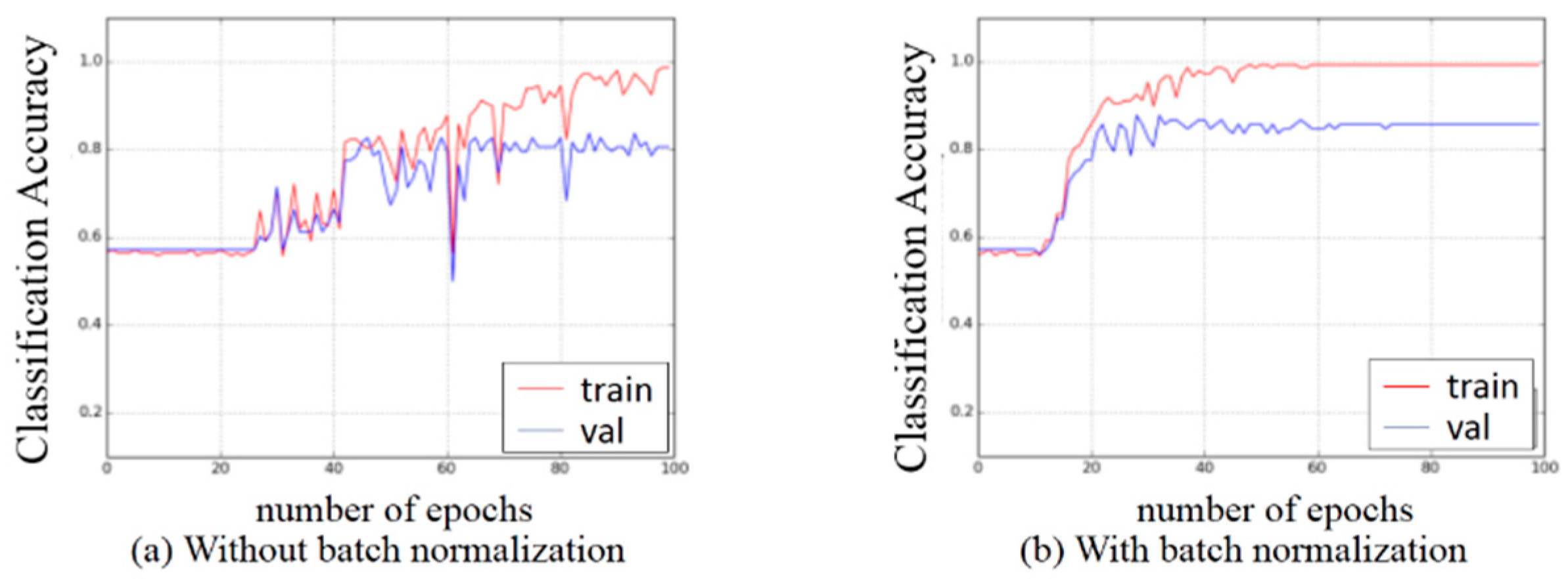
3.2. Experiments on Preprocessing

Figure 7a demonstrates the mean classification accuracy (MCA) curve of the training process without batch normalization. After that, batch normalization was performed on the input images, which set the mean and variance value of each channel (red, green, and blue channels in total) to 0.5 and 0.5. The training curve after batch normalization is demonstrated in Figure 7b. The comparison shows that using batch normalization can significantly accelerate the network training. In this case, we decided to use batch normalization as a preprocessing operation. However, from Figure 7a,b it can be observed that a risk of over fitting exists, which remains to be solved.

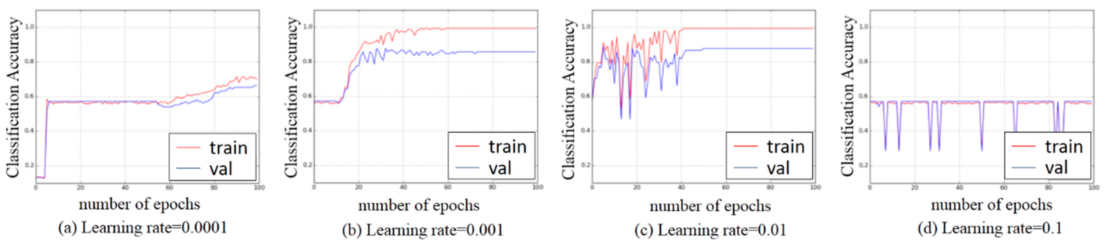
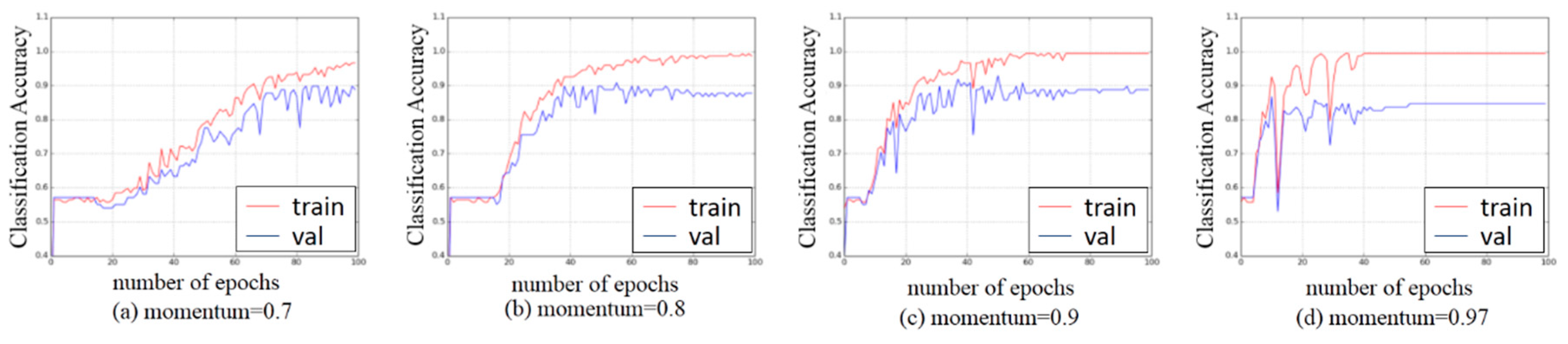
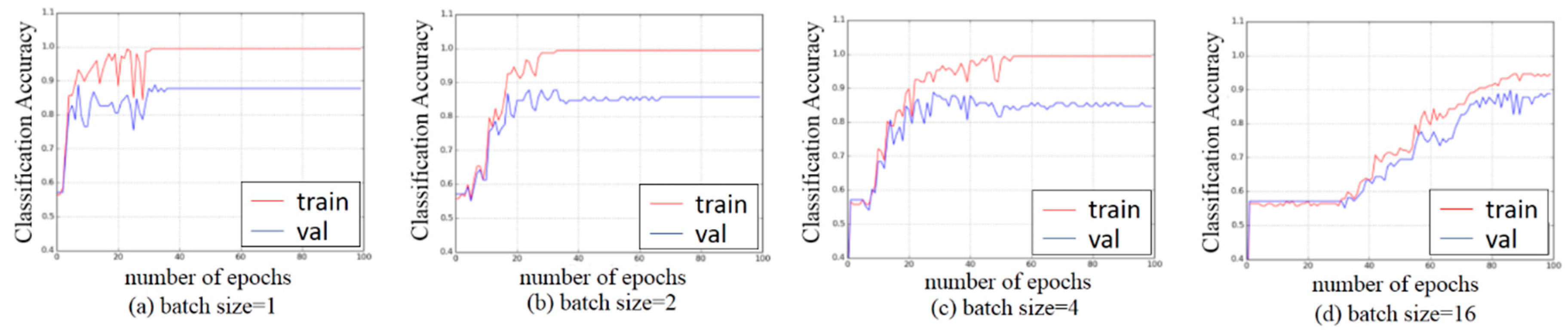
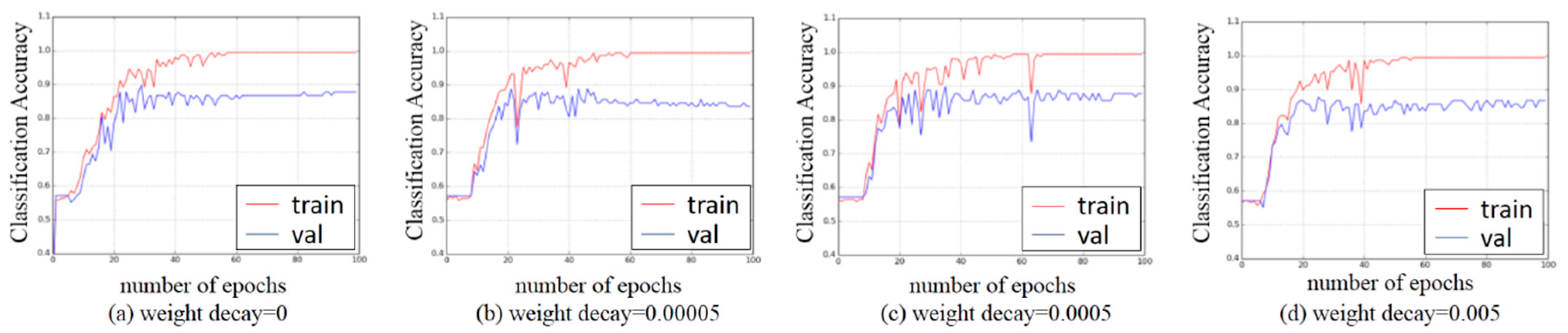
3.3. Experiments on Hyper-Parameters Tuning

Deep neural networks show great potential in many vision classification applications, but their final performance is strongly affected by the selection of hyper-parameters [35]. To obtain approximately optimal hyper-parameters, several experiments on hyper-parameters selection were conducted. Their impact was demonstrated via MCA curves on training samples and validation samples, as shown in Figure 8, Figure 9, Figure 10 and Figure 11. In each figure, one hyper-parameter was changed while the others were kept constant.

The performance of different learning rates is shown in Figure 8. From Figure 8, it can be observed that a too-small learning rate slows down the convergence of the cost function, as shown in Figure 8a, while a too-large learning rate leads to the neural network divergence. A better classification performance can be obtained by choosing an appropriate learning rate, as shown in Figure 8b.

The classifier performance of different momentums is shown in Figure 9. It can be observed that appropriately increasing the momentum coefficient can well accelerate the convergence of the cost function. However, using a too-large momentum coefficient (0.97) destabilizes the training process at the initial stages. A better selection of the momentum coefficient is shown in Figure 9b,c.

The performance of different batch sizes is shown in Figure 10. It can be observed that a too-small batch size can cause oscillation at initial stages, as shown in Figure 10a. However, a too-large batch size slows down the learning process and degrades the classification accuracy, as shown in Figure 10d. A better classifier performance can be obtained by using an appropriate batch size, as shown in Figure 10b,c.

The performance of different weight decays are shown in Figure 11. From Figure 11, it can be observed that using weight decay has no impact on improving the classifier performance. In this case, we decided not to use weight decay in this study. After hyper-parameter tuning, the selected hyper-parameter values are shown in

Table 4. Hyper-parameters obtained.

Hyper-parameter	Learning Rate	Momentum	Batch Size	Weight Decay
Value	0.001	0.9	4	0

.

3.4. Comparison with Other Methods

In comparison with the CNN methods, four more algorithms for HLB disease category classification were explored. For the first comparison algorithm, only the color histogram was used for feature extraction, and SVM was applied for multi-class classification. For the second comparison algorithm, only the LBPH method was used for feature extraction and the SVM for multi-class classification. The radius and sampling points were set to 1 and 8, respectively. For the third comparison algorithm, only eight vegetation indices were computed as feature vector and SVM was used as the classifier. For the fourth comparison algorithm, the color histogram, LBPH, and vegetation indices were concatenated as the feature vector, which was used for SVM classification. For all the SVM models, the radial basis function (RBF) was chosen as the kernel function. The penalty parameter was set to 1.0, and the “one against one” strategy was used for multi-class classification.

To evaluate the performance of different methods, overall accuracy (OA) and standard error (SE) were calculated, which were used to measure the classification accuracy and the standard deviation of the experimental results [36]. In our experiments, the training and validation samples were randomly selected from our dataset (Table 3). To minimize the effects of randomness, the sample selection and classification were iterated for 10 times. The quantified measurement of OA, SE, and confusion matrix for 10 consecutive experiments were recorded and averaged. The final OA and SE are shown in

Table 5. Comparison of overall accuracy (OA) and standard error (SE) of different methods on the validation set.

Method	OA (%)	SE (%)
Color Histogram + SVM	85.92	1.31
LBPH + SVM	65.10	2.86
VI + SVM	87.65	1.17
Color Histogram + LBPH + VI + SVM	90.00	0.96
CNN	91.43	0.83

, and its corresponding confusion matrix is demonstrated in

Table 6. Confusion matrix of different methods.

Method	GT/Predicted Class	Normal (%)	Light (%)	Medium (%)
Color Histogram + SVM	normal	89.11	10.89	0.00
	light	13.79	84.48	1.72
	medium	2.31	22.31	75.38
LBPH + SVM	normal	98.57	1.43	0.00
	light	72.07	27.59	0.34
	medium	48.46	46.92	4.62
VI + SVM	normal	88.39	11.61	0.00
	light	8.97	88.62	2.41
	medium	0.77	16.92	82.31
Color Histogram + LBPH + VI + SVM	normal	94.33	5.67	0.00
	light	9.16	89.28	1.56
	medium	1.80	21.48	76.72
CNN	normal	93.93	6.07	0.00
	light	7.93	88.62	3.45
	medium	0.00	13.08	86.92

.

From Table 5, it can be observed that the LBPH + SVM approach results in low accuracy. The reason for this result is that the texture features of different categories shared little difference. However, the Color Histogram + SVM approach achieved higher accuracy, since the color difference of different categories was more obvious, as can be observed from Figure 6. The VI + SVM approach obtained an approximate performance with the Color Histogram method since the mathematic computation on different color channels (vegetation index) can be regarded as another kind of color information. The Color Histogram + LBPH + VI + SVM approach further increased the accuracy, since extra effective features help to improve the classification. Experimental results showed that the CNN method achieved the highest OA and lowest SE, which outperformed other methods in terms of accuracy and stabilization. On the other hand, for the recognition of the diseased samples, the CNN method significantly outperformed others, as shown in Table 6. One possible reason for this result was that the CNN emphasis automatic feature learning, which may combine the color and texture features and extract better features for the classification stage.

4. Conclusions

In this study, the UAV data collection and concurrent ground investigation were conducted in two wheat fields. The UAV data were analyzed, and its relationship with HLB disease category was investigated. A CNN was applied for HLB disease category classification. The experiments on data preprocessing, classification, and hyper-parameters tuning were conducted. Besides CNN, the performance of traditional approaches was evaluated. Color and texture features, as well as vegetation indices, were extracted as hand craft features, and SVM was applied as the classifier. Experimental results showed that the overall accuracy and standard error of the CNN method was 91.43% and 0.83%, which outperformed other methods in terms of accuracy and stabilization. The experimental results in this study demonstrated that the UAV remote sensing can be an effective tool for HLB disease detection. However, other pathologies may also cause similar symptoms as HLB disease. In our current research, it is unfeasible to distinguish different kinds of disease infection. In the future work: (1) We will collect the UAV data of other diseases and build an effective classifier, and (2) we plan to add extra data and use transfer learning to overcome the problem of over fitting.

References

1. Zhu, X.; Chang, N.; Zhou, C. Advance of research in helminthosporium leaf blotch of wheat. Agric. Sci. Technol. Equip. 2010, 08, 15–18. [Google Scholar]
2. Saari, E.E. Leaf blight disease and associated soil-borne fungal pathogens of wheat in South and South East Asia. Helminthosporium Blights Wheat Spot Blotch Tan Spot 1998, 37–51. [Google Scholar]
3. Sharma, R.C.; Duveiller, E. Effect of helminthosporium leaf blight on performance of timely and late-seeded wheat under optimal and stressed levels of soil fertility and moisture. Field Crops Res. 2004, 89, 205–218. [Google Scholar] [CrossRef]
4. Huang, H.; Lan, Y.; Deng, J.; Yang, A.; Deng, X.; Zhang, L.; Wen, S. A semantic labeling approach for accurate weed mapping of high resolution UAV imagery. Sensors 2018, 18, 2113. [Google Scholar] [CrossRef] [PubMed]
5. Huang, H.; Deng, J.; Lan, Y.; Yang, A.; Deng, X.; Wen, S.; Zhang, H.; Zhang, Y. Accurate weed mapping and prescription map generation based on fully convolutional networks using UAV imagery. Sensors 2018, 18, 3299. [Google Scholar] [CrossRef]
6. Peña, J.; Torressánchez, J.; Serranopérez, A.; Lópezgranados, F. Weed mapping in early-season maize fields using object-based analysis of unmanned aerial vehicle (UAV) images. PLoS One 2013, 8, e77151. [Google Scholar] [CrossRef] [PubMed]
7. Huang, H.; Deng, J.; Lan, Y.; Yang, A.; Deng, X.; Zhang, L.; Wen, S.; Jiang, Y.; Suo, G.; Chen, P. A two-stage classification approach for the detection of spider mite- infested cotton using UAV multispectral imagery. Remote Sens. Lett. 2018, 9, 933–941. [Google Scholar] [CrossRef]
8. Franke, J.; Menz, G. Multi-temporal wheat disease detection by multi-spectral remote sensing. Precis. Agric. 2007, 8, 161–172. [Google Scholar] [CrossRef]
9. Albetis, J.; Duthoit, S.; Guttler, F.; Jacquin, A.; Goulard, M.; Poilvé, H.; Féret, J.B.; Dedieu, G. Detection of flavescence dorée grapevine disease using unmanned aerial vehicle (UAV) multispectral imagery. Remote Sens. 2017, 9, 308. [Google Scholar] [CrossRef]
10. Mirik, M.; Jones, D.C.; Price, J.A.; Workneh, F.; Ansley, R.J.; Rush, C.M. Satellite remote sensing of wheat infected by Wheat streak mosaic virus. Plant Dis. 2011, 95, 4–12. [Google Scholar] [CrossRef]
11. Huang, W.; Lamb, D.W.; Niu, Z.; Zhang, Y.; Liu, L.; Wang, J. Identification of yellow rust in wheat using in-situ spectral reflectance measurements and airborne hyperspectral imaging. Precis. Agric. 2007, 8, 187–197. [Google Scholar] [CrossRef]
12. Lan, Y.B.; Chen, S.D.; Fritz, B.K. Current status and future trends of precision agricultural aviation technologies. Int. J. Agric. Biol. Eng. 2017, 10, 1–17. [Google Scholar]
13. Leng, W.F.; Wang, H.G.; Xu, Y.; Ma, Z.H. Preliminary study on monitoring wheat stripe rust with using UAV. Acta Phytopathol. Sin. 2012, 42, 202–205. [Google Scholar]
14. Wei, L.; Cao, X.; Fan, J.R.; Wang, Z.; Yan, Z.; Yong, L.; West, J.S.; Xu, X.; Zhou, Y. Detecting wheat powdery mildew and predicting grain yield using unmanned aerial photography. Plant Dis. 2018, 12–17. [Google Scholar]
15. López-Granados, F.; Torres-Sánchez, J.; Serrano-Pérez, A.; de Castro, A.I.; Mesas-Carrascosa, F.J.; Peña, J. Early season weed mapping in sunflower using UAV technology: variability of herbicide treatment maps against weed thresholds. Precs. Agric. 2016, 17, 183–199. [Google Scholar] [CrossRef]
16. LeCun, Y.; Bengio, Y.; Hinton, G. Deep learning. Nature 2015, 521, 436–444. [Google Scholar] [CrossRef] [PubMed]
17. Ioffe, S.; Szegedy, C. Batch normalization: accelerating deep network training by reducing internal covariate shift. arXiv, 2015; arXiv:1502.03167. [Google Scholar]
18. Boureau, Y.L.; Bach, F.; Lecun, Y.; Ponce, J. Learning Mid-Level Features for Recognition. In Proceedings of the 2010 IEEE Computer Society Conference on Computer Vision and Pattern Recognition (2010), San Francisco, CA, USA, 13 June–18 June 2010. [Google Scholar]
19. Bejiga, M.; Zeggada, A.; Nouffidj, A.; Melgani, F. A convolutional neural network approach for assisting avalanche search and rescue operations with UAV imagery. Remote Sens. 2017, 9, 100. [Google Scholar] [CrossRef]
20. Ammour, N.; Alhichri, H.; Bazi, Y.; Benjdira, B.; Alajlan, N.; Zuair, M. Deep learning approach for car detection in UAV imagery. Remote Sens. 2017, 9, 312. [Google Scholar] [CrossRef]
21. Längkvist, M.; Kiselev, A.; Alirezaie, M.; Loutfi, A. Classification and segmentation of satellite orthoimagery using convolutional neural networks. Remote Sens. 2016, 8, 329. [Google Scholar] [CrossRef]
22. Lecun, Y.; Kavukcuoglu, K.; Farabet, C.M. Convolutional networks and applications in vision. In Proceedings of the 2010 IEEE International Symposium on Circuits and Systems, Paris, France, 30 May–2 June 2010. [Google Scholar]
23. Krizhevsky, A.; Sutskever, I.; Hinton, G.E. ImageNet Classification with Deep Convolutional Neural Networks. In Proceedings of the International Conference on Neural Information Processing Systems, Lake Tahoe, Nevada, 3–8 December 2012. [Google Scholar] [CrossRef]
24. Swain, M.J.; Ballard, D.H. Indexing via color histograms. In Proceedings of the 2010 IEEE International Symposium on Circuits and Systems, Osaka, Japan, 4–7 December 1990. [Google Scholar]
25. Ojala, T.; Harwood, I. A comparative study of texture measures with classification based on feature distributions. Pattern Recognit. 1996, 29, 51–59. [Google Scholar] [CrossRef]
26. Ahonen, T.; Hadid, A.; Pietikainen, M. Face description with local binary patterns: Application to face recognition. IEEE Trans. Pattern Anal. Mach. Intell. 2006, 12, 2037–2041. [Google Scholar]
27. Meyer, G.E.; Neto, J.C. Verification of color vegetation indices for automated crop imaging applications. Comput. Electron. Agric. 2008, 63, 282–293. [Google Scholar] [CrossRef]
28. Hunt, E.R.; Cavigelli, M.; Daughtry, C.S.T.; Mcmurtrey, J.E.; Walthall, C.L. Evaluation of digital photography from model aircraft for remote sensing of crop biomass and nitrogen status. Precis. Agric. 2005, 6, 359–378. [Google Scholar] [CrossRef]
29. Wang, X.; Wang, M.; Wang, S.; Wu, Y. Extraction of vegetation information from visible unmanned aerial vehicle images. Trans. Chin. Soc. Agric. Eng. 2015, 31, 152–159. [Google Scholar]
30. Sun, G.; Wang, X.; Yan, T.; Xue, L.; Man, C.; Shi, Y.; Chen, J.; University, N.A. Inversion method of flora growth parameters based on machine vision. Trans. Chin. Soc. Agric. Eng. 2014, 30, 187–195. [Google Scholar]
31. Louhaichi, M.; Borman, M.; Johnson, D. Spatially located platform and aerial photography for documentation of grazing impacts on wheat. Geocarto Int. 2001, 16, 65–70. [Google Scholar] [CrossRef]
32. Gamon, J.A.; Surfus, J.S. Assessing leaf pigment content and activity with a reflectometer. New Phytol. 2010, 143, 105–117. [Google Scholar] [CrossRef]
33. Suykens, J.A.K. Support vector machines: A nonlinear modelling and control perspective. Eur. J. Control. 2001, 7, 311–327. [Google Scholar] [CrossRef]
34. Chi, M.; Feng, R.; Bruzzone, L. Classification of hyperspectral remote-sensing data with primal SVM for small-sized training dataset problem. Adv. Space Res. 2008, 41, 1793–1799. [Google Scholar] [CrossRef]
35. Domhan, T.; Springenberg, J.T.; Hutter, F. Speeding up automatic hyperparameter optimization of deep neural networks by extrapolation of learning curves. In Proceedings of the 24th International Conference on Artificial Intelligence, Buenos Aires, Argentina, 25–31 July 2015. [Google Scholar]
36. Guggenmoos-Holzmann, I. The meaning of kappa: probabilistic concepts of reliability and validity revisited. J. Clin. Epidemiol. 1996, 49, 775–782. [Google Scholar] [CrossRef]
Figure 1. General overview of the study location.
Applsci 09 00558 g001
Figure 2. Phantom 4 in our experimental field
Applsci 09 00558 g002
Figure 3. The distribution of ground control point makers in the HLB field.
Applsci 09 00558 g003
Figure 4. Disease severity categories established to represent the wheat health state.
Applsci 09 00558 g004
Figure 5. The architecture of our convolutional neural networks (CNN) for Helminthosporium leaf blotch (HLB) disease classification. In the first module, batch normalization is performed to the input image. In the second module, feature extraction is applied to the normalized image. In this section, convolutional layer and max-pooling layer is abbreviated as C and P, respectively. C1:6@96 × 96 means this is the first layer, and it is a convolutional layer composed of six feature maps, each of which is in size of 96 × 96. In the third module, three fully connected layers are used for classification. In this section, fully connected layer is abbreviated as F. For example, F5:120 means this is a full connection layer. It is the fifth layer and has 120 neurons.
Applsci 09 00558 g005
Figure 6. Field images in different HLB disease categories.
Applsci 09 00558 g006
Figure 7. Comparison of performance with and without batch normalization. (a) Without batch normalization; (b) With batch normalization.
Applsci 09 00558 g007
Figure 8. Comparison of classifier performance on different learning rates. (a) Learning rate = 0.0001; (b) Learning rate = 0.001; (c) Learning rate = 0.01; (d) Learning rate = 0.1.
Applsci 09 00558 g008
Figure 9. Comparison of classifier performance of different momentums. (a) momentum = 0.7; (b) momentum = 0.8; (c) momentum = 0.9; (d) momentum = 0.97.
Applsci 09 00558 g009
Figure 10. Comparison of classifier performance of different batch sizes. (a) batch size = 1; (b) batch size = 2; (c) batch size = 4; (d) batch size = 16.
Applsci 09 00558 g010
Figure 11. Comparison of classifier performance of different weight decays. (a) weight decay = 0; (b) weight decay = 0.00005; (c) weight decay = 0.0005; (d) weight decay = 0.005.
Applsci 09 00558 g011