Article

Solving the Time-Varying Inverse Kinematics Problem for the Da Vinci Surgical Robot

State Key Laboratory of Mechanical Transmission, Chongqing University, Chongqing 400044, China
*
Author to whom correspondence should be addressed.
Appl. Sci. 2019, 9(3), 546; https://doi.org/10.3390/app9030546
Submission received: 15 November 2018 / Revised: 29 January 2019 / Accepted: 3 February 2019 / Published: 6 February 2019
(This article belongs to the Special Issue Advanced Mobile Robotics)

Abstract

:

Featured Application

The work of this paper is mainly applied for the inverse kinematics solving of Da Vinci surgical robot and its similar robotic systems that do not satisfy the Pieper principle.

Abstract

A dialytic-elimination and Newton-iteration based quasi-analytic inverse kinematics approach is proposed for the 6 degree of freedom (DOF) active slave manipulator in the Da Vinci surgical robot and other similar systems. First, the transformation matrix-based inverse kinematics model is derived; then, its high-dimensional nonlinear equations are transformed to a high-order nonlinear equation with only one unknown variable by using the dialytic elimination with a unitary matrix. Finally, the quasi-analytic solution is eventually obtained by the Newton iteration method. Simulations are conducted, and the result show that the proposed quasi-analytic approach has advantages in terms of accuracy (error < 0.00004 degree (or mm)), solution speed (<20 ms) and is barely affected by the singularity during intermediate calculations, which proves that the approach meets the real-time and high-accuracy requirements of master–slave mapping control for the Da Vinci surgical robots and other similar systems. In addition, the proposed approach can also serve as a design reference for other types of robotic arms that do not satisfy the Pieper principle.

Graphical Abstract

1. Introduction

In recent years, medical robots have increasingly been used as fundamental surgical instrument/equipment [1], among which the Da Vinci system developed by Intuitive Surgical Company is the most successful [2]. The Da Vinci robotic system consists of three components: the surgeon console (master manipulators), the patient trolley (slave manipulators), and the imaging system [3]. The surgeon manipulates two master handles at the master remote console, which can acquire high-resolution, binocular, three-dimensional, magnified views of the operative field as compared with open surgery [4]. However, this kind of master–slave operation mode poses a great challenge to the real-time and accurate performance of the master–slave mapping control, among which the inverse kinematics problem is the first obstacle. The Da Vinci system and similar surgical robot systems satisfy the following two features:
(1)
contain mechanical structures to generate Remote Center of Motion [5] (RCM, a fixed point on the active arm, there are two methods to generate RCM based motion: (a) virtual RCM, (b) physically constrained RCM [6]), and the structure can be simplified;
(2)
do not satisfy the Pieper principle.
At present, the main methods of robotic inverse kinematics include the analytic method and the numerical method. The analytic approach uses vector, spinor or Lie algebra to obtain results [7,8,9], which can only obtain satisfied solutions in limited robotic configurations that should satisfy the Pieper principle [10,11], etc. However, to imitate the surgeon operation, the manipulators of most thoracic and abdominal surgery robots, including the Da Vinci system, contain rotational/translational kinematic pairs, tilt angle joints, and offset joints at the tip (artificial wrist part) that are designed for additional flexibility, which is beyond the solution capability of the analytic approach.
One feasible strategy is to simplify the kinematic model to acquire analytical results. For example, Ai et al. and Podsedkowski et al. [12,13] obtained an approximate solution by separating the position and orientation of the slave manipulators, the solution deviation of which needs to be manually eliminated by experienced surgeons via visual inspection. Zhang et al. [14] solved the inverse kinematics of a 4-DOF surgical robot using the elimination method, and Mezouar et al. [15] used unit dual quaternions to model the kinematics, however, outcomes of their studies benefited strongly from the simplicity of the arm configuration. In addition, Fu et al. [16,17] obtained an approximate solution based on the differential transformation that increases error feedbacks to compensate the cumulative error, the final precision of which can reach 0.18 mm.
Another way to solve the inverse kinematics problem of the surgical robot that does not satisfy the Pieper principle is the Jacobian matrix-based numerical method [18]. However, this method involves a Jacobian matrix, which may lose versatility due to its singularity problem as well as the low convergence speed of the iterative solutions. To improve the numerical solution performance, a numerical method based on the position increment of robotic joints was proposed [18]. Specifically, to make this method suitable for the inverse kinematics analysis of a robotic manipulator with an offset wrist, Bu et al. [19] used the method of decoupling DOFs based on a cut-off point that is limited by the manipulator configuration. In addition, modern methods such as the neural network method [20], the genetic algorithm [21], the electromagnetism-like mechanism [22,23], the hybrid electromagnetism-like mechanism [24], etc., have been gradually explored for possible solutions of the inverse kinematics of surgical robots. However, these methods either require a large amount of sample data or suffer from poor convergence speed; therefore, these methods are not suitable for the rapid development of a master–slave manipulator in surgical robots.
To address the lack of efficient and accurate inverse kinematics solutions for the Da Vinci system, we propose a quasi-analytic solution method that involves dialytic elimination and the Newton iteration method. The dialytic elimination method [25] is used to transform the high-dimensional equations into a nonlinear equation containing only one unknown variable, which is then solved by the Newton iteration method. In applying this method to the inverse kinematics solution of slave manipulator, we show dual superiorities: (a) barely affected by the singularity problem and (b) maintain rapidity.
The steps of our proposed method as follows:
(1)
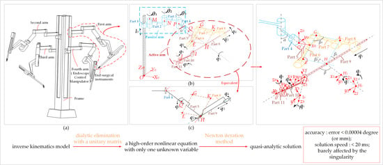
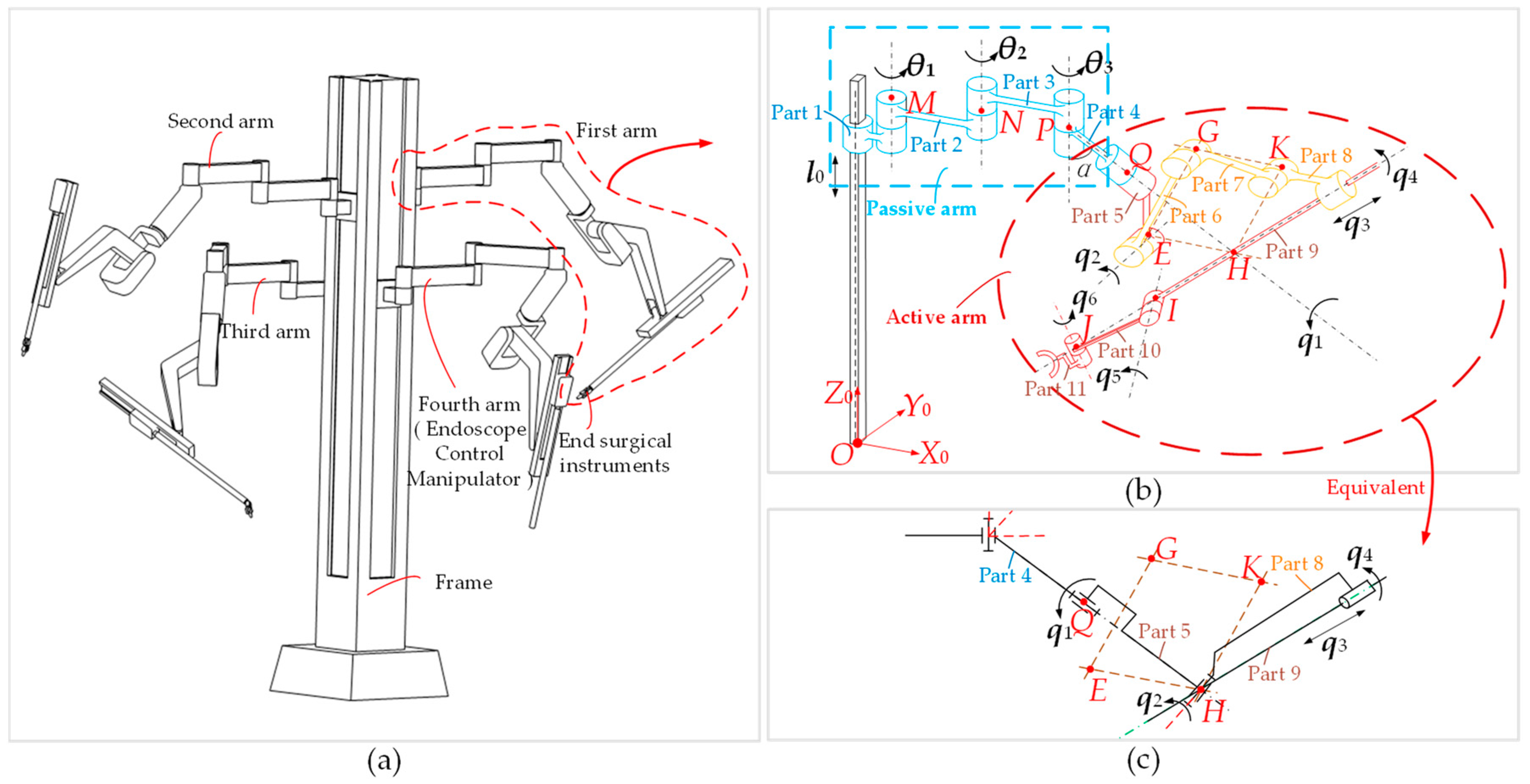
simplify the structure of RCM, using an equivalent mechanism to take the place of the RCM mechanism.
(2)
establish the coordinate system, this step can be realized by the D–H (Denavit–Hartenberg) method or combine the characteristics of the structure to make sure there are more origins of the coordinate system can be set up at the same point.
(3)
obtain the mathematical model of forward and inverse kinematics via the matrix transformation method. Then, transform the high-dimensional equations into a nonlinear equation containing only one unknown parameter using the dialytic elimination method, and solve it by the Newton iteration method.
The rest of this paper is organized as follows: Section 2 presented the kinematics analysis of the Da Vinci system; Section 3 solves the inverse kinematics by the Newton iteration method; Section 4 analyzes our solution and compared it with other methods via a simulation; Section 5 concludes the paper.

2. Kinematics Analysis

2.1. Forward Kinematics Analysis

During surgery using the Da Vinci medical robot, dual articulated arms (slave manipulators) work as the right and left hand of the surgeon, respectively. The coordinate frame of the master/slave manipulator is set the same as the coordinate frame of human sight, i.e., the world coordinate frame. Therefore, in Figure 1, the origin of the base coordinate frame of the slave manipulator is located at the bottom of the robot frame. The Z0-axis is upward, along the robot frame.
Before surgery, the angles of passive joints M, N, and P and the position of the M joint on the frame are adjusted manually and then remain fixed during surgery. The joints that mainly assist the surgeon are the active joints of the slave manipulator: Q, E, G, K, H, I, and J in Figure 1b.
The DOFs of the slave manipulator includes four DOFs: l0, θ1, θ2 and θ3. The parts 6, 7, and 8 in the active arm belong to the parallelogram mechanism (i.e., these three parts cannot move freely but under the motion constraint of the parallelogram mechanism in Figure 1c. Then only parts 4, 5, 8 and 9 can move freely in the slave manipulator, i.e., part 5 rotates around part 4, there is rotation between part 6 and part 5, and there is rotation between part 9 and part 8. Therefore, the entire slave manipulator will have 6 DOFs when the additional 3 DOFs of the H joint are considered.

2.2. Mathematical Model of Forward Kinematics

According to the previous analysis, an active arm coordinate system is established in Figure 2. The origin of the base coordinate x0y0z0 (0-coordinate frame) of the active arm is established at the joint Q between the passive and active arms, the direction of which is the same as that of the frame coordinate X0Y0Z0.
Figure 2 shows the six DOFs of the active arm in the slave manipulator, namely five rotating joints: q1, q2, q4, q5, q6, and a translational joint: q3.
Six transform matrixes frame from x1y1z1 (1-coordinate frame) to x6y6z6 (6-coordinate frame) can be obtained as follows:
{ T = { ( π α ) } x { q 1 } z { l Q H } z 2 1 T = { ( β π 2 ) } x { π 2 } y { q 2 } z 3 2 T = { q 3 } y 4 3 T = { π 2 } x { q 4 } z 5 4 T = { π 2 } x { q 5 } z 6 5 T = { l I J } y { π 2 } y { q 6 } z ,
where ijT means transform matrix from the i-coordinate frame to the j-coordinate frame; { }x, { }y and { }z represent the rotation angle around the x-axis, y-axis and z-axis, respectively; { }x, { }y and { }z denotes the translational movement along the x-axis, y-axis and z-axis, respectively.
Then, the pose matrix of the active arm at the endpoint of the slave manipulator can be obtained as follows:
T 6 0 = T 1 0 T 2 1 T 3 2 T 4 3 T 5 4 T 6 5 = [ n x o x a x p x n y o y a y p y n z o z a z p z 0 0 0 1 ] = [ R P 0 1 ] ,
where R and P are the orientation and position of the slave manipulator endpoint, respectively. Substituting Equation (1) into Equation (2) yields Equation (3):
T 6 0 = { ( π α ) } x { q 1 } z { l Q H } z { ( β π 2 ) } x { π 2 } y { q 2 } z { q 3 } y { π 2 } x { q 4 } z { π 2 } x { q 5 } z { l I J } y { π 2 } y { q 6 } z .

2.3. Mathematical Model of Inverse Kinematics

In the case of inverse kinematics, the known pose matrix is 06T in Equation (3), and the unknowns are q1, q2, q3, q4, q5 and q6.
Left-multiplying the matrices T = { q 3 } y 1 { q 2 } z 1 { π 2 } y 1 { ( β π 2 ) } x 1 { l Q H } z 1 { q 1 } z 1 { ( π α ) } x 1 on both sides of Equation (3) yields Equation (4):
T T 6 0 = { π 2 } x { q 4 } z { π 2 } x { q 5 } z { l I J } y { π 2 } y { q 6 } z .
To simplify the complexity of the formula, we construct a unitary matrix [26] U as follows. After introducing the matrix U, the variables in the 06T can be replaced by the Euler formula.
U = [ 1 2 i 1 2 i 0 0 1 2 1 2 0 0 0 0 1 0 0 0 0 1 ]
In addition, we know that E = U−1U. Left-multiply the inverse of unitary matrix U−1 and right-multiply the matrix U on both sides of Equation (4). Then, multiply the E matrix between these two matrices to transform Equation (4) into the following:
Y 3 X 2 C 1 X 1 C 2 C 3 = C 4 X 4 C 5 X 5 C 6 X 6 .
Here, C1 = U−1[{lQH}z{π/2 − β}z]−1U, C2 = U−1[{α − π}x]−1U, C3 = U−106TU, C4 = U−1{−π/2}zU, C5 = U−1{π/2}zU, and C6 = U−1{lIJ}y{π/2}yU. Clearly, C1, C2, C3, C4, C5 and C6 are constant matrices or parameter matrices related to the structure of the robot. In addition, Xj (j = 1, 2, 4, 5, 6) is as follows:
X j = { T X j 1 j = 1 , 2 T X j j = 4 , 5 , 6 ,
where TXj (j = 1, 2, 4, 5, 6) represents the results of the transform matrix of qj rotating around the z-axis, which undergoes the left-multiplication of U−1 and right-multiplication of U. Let xj = cos(qj) + isin(qj), xj−1 = cos(qj) − isin(qj); thus, TXj can be expressed as follows:
T X j = U 1 { q i } z U = [ x j 0 0 0 0 x j 1 0 0 0 0 1 0 0 0 0 1 ] .
Let Yj represents the result of the transform matrix qj along the y-axis, which undergoes the left-multiplication of U−1 and right-multiplication of U, and xj = qj; then, Yj can be expressed as follows:
Y j = U 1 { q i } y U = [ 1 0 0 2 2 x j 0 1 0 2 2 x j 0 0 1 0 0 0 0 1 ] .
Take A = Y 3 X 2 C 1 X 1 C 2 C 3 , B = C 4 X 4 C 5 X 5 C 6 X 6 . Then the dimensions of matrix A and matrix B are both 4 × 4. Each element in matrix A is a function containing x1, x2, and x3, while the elements in matrix B are functions containing x4, x5, and x6. In addition, corresponding elements in matrix A and matrix B are equal, i.e., Aij = Bij. The specific contents of the elements are detailed in Appendix A.
To realize element elimination, we evaluated elements in matrix A and B that do not contain x6 and x6−1: B13, B14, B23, B24, B33 and B34 to establish Equation (10):
A 13 = B 13 A 14 = B 14 A 23 = B 23 A 24 = B 24 A 33 = B 33 A 34 = B 34 } .
To further eliminate x4 and x5, the linear combination of x4 and x5, and their reciprocals are treated as new variables, i.e., X = [x4x5, x4x5−1, x4−1x5, x4−1x5−1, x4−1, x5−1, x4, x5, x40x50]T, which contains nine variables. Because there are only six equations in Equation (10), three more equations are required, which are attainable by conducting nonlinear computations on the elements in Equation (10), as shown in Equation (11).
A L 1 = A 34 A 23 + A 24 A 33 = B 34 B 23 + B 24 B 33 = B L 1 A L 2 = A 24 A 13 + A 14 A 23 = B 24 B 13 + B 14 B 23 = B L 2 A L 3 = A 13 A 34 + A 14 A 33 = B 13 B 34 + B 14 B 33 = B L 3 }
Then, by combining Equations (10) and (11):
[ D ( x 1 , x 2 , x 3 ) ] 9 × 9 X = 0 .
The matrix [D(x1, x2, x3)]9×9 contains only the variables x1, x2, and x3 since X is nonzero. The condition that Equation (12) has a solution is that the determinant of [D(x1, x2, x3)]9×9 equals zero. The following equation, which contains x1, x2, and x3, can be obtained provided that |D(x1, x2, x3)| = 0:
( C 1 x 1 + C 2 + C 3 x 1 1 ) x 2 = ( C 4 x 1 + C 5 + C 6 x 1 1 ) x 2 1 ,
where Cj is a constant related to the robot’s parameters. Considering that x1, x2, x4, x5, and x6 can be defined as xj = cos(qj) + isin(qj) and xj−1 = cos(qj) − isin(qj), then x1, x2, x4, x5, and x6 are all non-zero. Therefore, x2 can be expressed by x1 according to Equation (13):
x 2 2 = ( X 1 x 1 + C 2 + C 3 x 1 1 ) [ ( C 4 x 1 + C 5 + C 6 x 1 1 ) ] = f 1 ( x 1 ) .
To represent x3 by x1 and x2, we construct the equations AL4 = A23A14 + A13A24 + A33A34 and BL4 = B23B14 + B13B24 + B33B34. Let AL4 = BL4, then
( C 7 x 1 + C 9 + C 12 x 1 1 ) x 3 x 2 + ( C 8 x 1 + C 11 + C 13 x 1 1 ) x 3 x 2 1 + C 10 = 0 .
Equation (15) contains only three variables, x1, x2, and x3, therefore, x3 can be expressed by x1 and x2 as:
x 3 = f 2 ( x 1 , x 2 ) .
Because both AL2 and AL3 are functions of x1, x2 and x3, by combining AL2 = BL2 with AL3 = BL3, the following can be obtained:
[ x 4 x 4 1 ] = [ i l I J 2 i l I J i l I J 2 i l I J ] [ A L 2 A L 3 ] .
Therefore,
x 4 = i l I J A L 2 2 i l I J A L 3 = f 3 ( x 1 , x 2 , x 3 ) .
Similarly, by combining A13 = B13 and A14 = B14 with Equation (16), the following can be obtained:
[ x 5 x 5 1 ] = [ 2 ( A L 2 i l I J ) 2 i l I J ( A L 2 i l I J ) 2 i ( A L 2 l I J i ) 2 l I J ( A L 2 l I J i ) ] [ A 14 A 13 ] .
Therefore, x5 can be represented by x1, x2, and x3:
x 5 = 2 A 14 ( A L 2 i l I J ) 2 i l I J A 13 ( A L 2 i l I J ) = f 4 ( x 1 , x 2 , x 3 ) .
Combined with Equations (16) to (20) and A11 = B11, x6 can finally be represented by x1:
x 6 = ( b 1 i + b 2 ) x 1 x 2 1 + ( b 3 i + b 4 ) x 2 1 + ( b 5 i + b 6 ) x 1 1 x 2 1 1 8 x 5 x 4 + i 4 x 4 1 8 x 5 1 x 4 + 1 4 x 5 + 1 4 x 5 1 + 1 8 x 5 x 4 1 i 4 x 4 1 1 8 x 5 1 x 4 1 = f 5 ( x 1 ) ,
where bj is a constant related to the robot’s parameters.
From Equations (16) to (21), the variables x2, x3, x4, x5, and x6 can be represented with the variable x1. Let A24 and B24 be equal, then:
F ( x 1 ) = A 24 B 24 = 0 .
By solving Equation (22), x1 can be solved, then x2, x3, x4, x5, and x6 can be subsequently solved by Equation (16) to (21). Specifically, we know from Equation (14) that x 2 = ± f 1 ( x 1 ) , therefore, F(x1) will have two expressions:
F ( ξ 1 ) = { F 1 ( x 1 ) x 2 = f 1 ( x 1 ) F 2 ( x 1 ) x 2 = f 1 ( x 1 ) .
Equation (23) will be electively solved according to the minimum norm of the distance the joint moved.

3. Inverse Kinematics Solution

From the derivation of the forward and inverse kinematics of the Da Vinci slave manipulator, it is known that the key to solving inverse kinematics is to solve the nonlinear Equation (22).

3.1. Inverse Kinematics Solution Method

The Newton–Raphson method is an efficient numerical iterative approach to solve nonlinear equations in real and complex domains. In this paper, we construct the following iterative formula:
x n + 1 = x n F ( x n ) F ( x n ) .

3.2. Initial Value of the Inverse Kinematics Solution

The motion ranges of each joint in the Da Vinci slave manipulator are as follows: θ1 from −90° to 90°, θ2 from −135° to 0°, lIH from 0 to 315 mm, θ3 from −180° to 180°, θ4 from −90° to 90°, and θ5 from −90° to 90°. In the previously defined x1 = cos(q1) + isin(q1), q1 is the rotation angle of the first joint with a range of [−π/2, π/2]. A finite number of values are obtained by extracting values within these available ranges at a certain angle interval (our subsequent calculation results show that a less than 5 ° angle interval is acceptable) to solve the forward kinematics, the results of which are stored as the initial value database for the inverse kinematics solution. By selecting the data from the initial value database that is the least squares approximate to the required inverse kinematics as the initial values, the Newton iteration method will successfully converge.

3.3. Inverse Kinematics Solution Process

According to the inverse kinematics of the Da Vinci slave manipulator and the derived solution process, a detailed solution flow chart is constructed in Figure 3.
In Figure 3, Tend is the pose matrix at the endpoint of the robot (i.e., 06T), ε is the precision of the solution, θ0 is the initial value, h is the initial step value, and X_s represents the values of each joint at previous positions. The value k is used to determine whether both forms of F(x1) have been solved.

4. Example Analysis and Discussion

4.1. Parameters of the Da Vinci Slave Manipulator

According to Figure 4, the size parameters of the Da Vinci slave manipulator are shown in Table 1.

4.2. Solution of Proposed Method

As shown in Table 2 (the form is referenced by the book: An Introduction to Error Analysis [27]), the input values are a set of arbitrarily selected joint parameters within the effective range of joint space. The outputs in Table 2 are the calculated values by our proposed method. h represents the step size of the solution, and the error is calculated as follows:
ε = | Output Input | .
In this paper, the solution precision of the Newton–Raphson method is 1E–10 ε = 1E-7 for Tend, θ0 takes the minimum value of −90° within the feasible region, and the initial step size is h0 = 20°. The test carried on CodeBlocks 16.01 based on the hardware that a PC platform running with an Intel (R) Core (TM) i5-4460 CPU, clocked at 3.2 GHz (memory: 4 GB).
We also use the same input to run the procedure on the “R12CCPU-V” MELSEC iQ-R series C language controller from Mitsubishi Electric and VxWorks 6.9 operating system, the results are list in Table 3.
In order to verify the proposed method, we build a simulation model in Adams. Firstly, we gave a random movement for the simulation model, then we obtained the matrix of the end pose from the simulation result (Figure 5a), which included the position and the orientation. Secondly, the matrixes were imported to the algorithm we proposed as input. Thirdly, we used our solution to drive the robot model. In the final results, depicted in Figure 5b, we see that the curve obtained by our algorithm is very close to the target curve. This means the proposed method is of high accuracy.

4.3. Discussion of the Solution

As noted in the previous section, the main focus of the solution includes the solution accuracy, real-time performance (solution speed) and the singularity problem (based on the joint position solution or not).
(1) Solution accuracy
Table 2 shows that for any input joint parameter, whether an integer or a decimal value accurate to nine decimal places, the error between the calculated values (output) and the given values (input) of six joint parameters of the slave manipulator is within 0.00004 degree (or mm), which demonstrates that the proposed approach for the Da Vinci surgical robot inverse kinematics is capable of finding effective solutions with high accuracy.
(2) Solution speed
The number of calculation steps of the algorithm/program is one of the influential factors that affect the solution speed. As schematically shown in Figure 3, the number of steps of the inverse kinematics approach proposed in this paper depends mainly on two factors:
① The number of Newton iterations in the best-case scenario, the numerical solution can be obtained by one iteration when the initial value is perfectly selected. In general, if the given initial value ensures convergence, then the solution of F(x1) = 0 is expected to take approximate 20 iterations; in cases where the convergence fails, the program is designed to iterate at most 50 times and then exit to avoid a dead loop.
② The step size. when the step size h is large, the iteration times are reduced, thereby shorten the calculation time. However, the selection of initial values will be relatively imprecise, resulting in higher possibility of solution failure due to unreasonable initial values. In cases where the step size is small, the initial values tend to be more precise, resulting in a greater possibility of obtaining a solution. However, the resulting shortcoming is the demand for more calculation steps and longer time.
An improved calculation process is proposed by taking both factors into account: first, start the procedure by following the flow chart shown in Figure 3 with a relatively large step size; second, reduce the step size gradually for more precise initial values if the equation has no solution. This approach boosts the speed of calculation but also reduces the possibility of solution failure.
(3) Singularity influences
Our method abandons the use of Jacobian matrix inversion. Therefore, there will be barely no singular solution in the condition of a good initial value from a mathematical perspective. On the other hand, because our algorithm is based on the position increment of the manipulator’s joints, Then, the motion joint position trajectory is generated by interpolation based on the initial joint position and the end joint position. The joint position interpolation is not affected by the singularity.

4.4. Comparison with Other Methods

Table 4 compared our method with another two typical methods in applicability, complexity of calculation, solution precision, solution speed and singularity influences.
Particularly, we choose separates the position and orientation method (name as “separate P&R method” below) to applied on the Da Vinci slave manipulator, and the comparison with the proposed method within the same simulation model is shown in Figure 6. The position curve of “separate P&R method” is following the target with some fluctuation, while the orientation result is far away from the correct solution, which means that the Separate P&R method is not suitable for the slave manipulator that dissatisfied the Pieper principle. Even though increasing the error feedback to compensate for the results may increase the solution precision, the compensation operation will take a large amount of time, which proves the superiority of our proposed method in terms of solution precision and speed.

5. Conclusions

(1) In this paper, an inverse kinematics mathematical model of the 6-DOF active arm of the Da Vinci surgical robot established by using a coordinate transformation matrix method according to its mechanical motion diagram and working characteristics. By introducing a unitary matrix, the mathematical model on the real plane is transformed to a complex plane, consequently avoiding the relatively complex trigonometric calculations associated with the conventional solution procedure. Following the steps proposed, this approach can apply to other similar robot kinematic problems.
(2) The dialytic elimination method serves to individually eliminate the joint variables and ultimately obtains a high-order nonlinear equation with only one unknown variable of the first joint. Subsequently, the Newton iteration method is introduced to solve the nonlinear equation on the basis of selecting multiple initial values reasonably in the feasible region. The test shows that carefully changing the step size and selecting initial values in the feasible region for the iteration solution of the nonlinear equation will significantly reduce the possibility of solution failure.
(3) In theory, the accuracy of the approach can reach an error of < 0.00004 degree (or mm) and achieve a solution time of 0.5 s (Intel (R) Core i5-4460 CPU, clocked at 3.2 GHz (memory: 4 GB)). Running the procedure on better hardware and software (based on the “R12CCPU-V” MELSEC iQ-R series C language controller from Mitsubishi Electric and VxWorks 6.9 operating system) decreases the solution time to 20 ms, which fully satisfies the real-time performance requirement of surgical robots.
(4) A method that combines dialytic elimination and the Newton iteration method is applied to solve the inverse kinematics problem of the slave manipulators of the master–slave surgical robot. The proposed approach achieves higher accuracy than other solutions based on position and orientation separation while the real-time performance is satisfied. Moreover, in contrast to other numerical solutions, the solution method is based on the position of the joint and is therefore barely not affected by any singularity. Further, the application of our approach removes the restriction of the design of the master manipulator configuration.

Supplementary Files

Supplementary File 1

Author Contributions

Conceptualization, L.B. and J.Y.; methodology, X.C.; software, F.Z.; validation, J.Y., L.B., Y.S. and X.C.; formal analysis, J.Y.; investigation, P.J.; resources, F.L.; data curation, L.B.; writing—original draft preparation, J.Y.; writing—review and editing, L.B., X.C. and Y.S.; visualization, X.C.; supervision, L.B.; project administration, L.B.; funding acquisition, X.C.

Funding

This research was funded by the Special Cooperation Program for Higher Education Institutions Collaborative Innovation (grant no. KH2016006), the Foundation for Sci & Tech Research Project of Chongqing Science & Technology Commission (grant nos. cstc2016jcyjA0472, and cstc2017zdcy-zdzxX0007), the National Natural Science Foundation of China (grant nos. 51705050, and 51709023), and Fundamental Research Funds for the Central Universities (grant no. 2018CDGFJX0022, 2018CDQYHK0029).

Acknowledgments

The authors gratefully acknowledge Zixiang Zhang for his valuable support with language editing.

Conflicts of Interest

The authors declare no conflict of interest.

Appendix A.

A 11 = ( c 1 i + c 2 ) x 1 x 2 1 + ( c 3 i + c 4 ) x 2 1 + ( c 5 i + c 6 ) x 1 1 x 2 1 ;
A 12 = ( c 7 i + c 8 ) x 1 x 2 1 + ( c 9 i + c 10 ) 5 x 2 1 + ( c 11 i + c 12 ) x 1 1 x 2 1 ;
A 13 = ( c 13 i + c 14 ) x 1 x 2 1 + ( c 15 i + c 16 ) x 2 1 + ( c 17 i + c 18 ) x 1 1 x 2 1 ;
A 14 = ( c 19 i + c 20 ) x 1 x 2 1 + ( c 21 i + c 22 ) x 2 1 2 2 x 3 + ( c 23 i + c 24 ) x 1 1 x 2 1 ;
A 21 = ( c 25 i + c 26 ) x 1 x 2 + ( c 27 i + c 28 ) x 2 + ( c 29 i + c 30 ) x 2 x 1 1 ;
A 22 = ( c 31 i + c 32 ) x 1 x 2 + ( c 33 i + c 34 ) x 2 + ( c 35 i + c 36 ) x 2 x 1 1 ;
A 23 = ( c 37 i + c 38 ) x 1 x 2 + ( c 39 i + c 40 ) x 2 + ( c 41 i + c 42 ) x 2 x 1 1 ;
A 24 = ( c 43 i + c 44 ) x 1 x 2 + ( c 45 i + c 46 ) x 2 2 2 x 3 + ( c 47 i + c 48 ) x 2 x 1 1 ;
A 31 = ( c 49 i + c 50 ) x 1 + ( c 51 i + c 52 ) x 1 1 ;
A 32 = ( c 53 i + c 54 ) x 1 + ( c 55 i + c 56 ) x 1 1 ;
A 33 = ( c 57 i + c 58 ) x 1 + ( c 58 c 57 i ) x 1 1 ;
A 34 = ( c 59 i + c 60 ) x 1 + ( c 60 c 59 i ) x 1 1 ;
B 11 = 1 8 x 6 x 5 x 4 + i 4 x 6 x 4 1 8 x 6 x 5 1 x 4 + 1 4 x 6 x 5 + 1 4 x 6 x 5 1 + 1 8 x 6 x 5 x 4 1 i 4 x 6 x 4 1 1 8 x 6 x 5 1 x 4 1 ;
B 12 = 1 8 x 5 x 4 x 6 1 i 4 x 4 x 6 1 1 8 x 5 1 x 4 x 6 1 + 1 4 x 5 x 6 1 + 1 4 x 5 1 x 6 1 + 1 8 x 5 x 4 1 x 6 1 + i 4 x 4 1 x 6 1 1 8 x 5 1 x 4 1 x 6 1 ;
B 13 = i 2 8 x 5 x 4 i 2 8 x 5 1 x 4 i 2 4 x 5 + i 2 4 x 5 1 i 2 8 x 5 x 4 1 i 2 8 x 5 1 x 4 1 ;
B 14 = ( 2 8 x 5 x 4 2 8 x 5 1 x 4 + 2 4 x 5 + 2 4 x 5 1 + 2 8 x 5 x 4 1 2 8 x 5 1 x 4 1 ) l I J ;
B 21 = 1 8 x 6 x 5 x 4 i 4 x 6 x 4 + 1 8 x 6 x 5 1 x 4 + 1 4 x 6 x 5 + 1 4 x 6 x 5 1 1 8 x 6 x 5 x 4 1 + i 4 x 6 x 4 1 + 1 8 x 6 x 5 1 x 4 1 ;
B 22 = 1 8 x 6 1 x 5 x 4 + i 4 x 6 1 x 4 + 1 8 x 6 1 x 5 1 x 4 + 1 4 x 6 1 x 5 + 1 4 x 6 1 x 5 1 1 8 x 6 1 x 5 x 4 1 + i 4 x 6 1 x 4 1 + 1 8 x 6 1 x 5 1 x 4 1 ;
B 23 = i 2 8 x 5 x 4 + i 2 8 x 5 1 x 4 i 2 4 x 5 + i 2 4 x 5 1 + i 2 8 x 5 x 4 1 + i 2 8 x 5 1 x 4 1 ;
B 24 = ( 2 8 x 5 x 4 + 2 8 x 5 1 x 4 + 2 4 x 5 + 2 4 x 5 1 2 8 x 5 x 4 1 + 2 8 x 5 1 x 4 1 ) l I J ;
B 31 = 2 8 x 6 x 5 x 4 i 2 4 x 6 x 4 + 2 8 x 6 x 5 1 x 4 + 2 8 x 6 x 5 x 4 1 i 2 4 x 6 x 4 1 2 8 x 6 x 5 1 x 4 1 ;
B 32 = 2 8 x 6 1 x 5 x 4 + i 2 4 x 6 1 x 4 + 2 8 x 6 1 x 5 1 x 4 + 2 8 x 6 1 x 5 x 4 1 + i 2 4 x 6 1 x 4 1 2 8 x 6 1 x 5 1 x 4 1 ;
B 33 = i 4 x 5 x 4 + i 4 x 5 1 x 4 i 4 x 5 x 4 1 i 4 x 5 1 x 4 1 ;
B 34 = ( 1 4 x 5 x 4 + 1 4 x 5 1 x 4 + 1 4 x 5 x 4 1 1 4 x 5 1 x 4 1 ) l I J , where ci is a function related to the structural parameters of the robot, which is known and can be regarded as a constant.

References

  1. Taylor, R.H. A Perspective on Medical Robotics. Proc. IEEE 2006, 94, 1652–1664. [Google Scholar] [CrossRef]
  2. Turchetti, G.; Palla, I.; Pierotti, F.; Cuschieri, A. Economic evaluation of Da Vinci-assisted robotic surgery: A systematic review. Surg. Endosc. 2012, 26, 598. [Google Scholar] [CrossRef] [PubMed]
  3. Pugin, F.; Bucher, P.; Morel, P.; Bucher, P.; Morel, P. History of robotic surgery: From AESOP and ZEUS to Da Vinci. J. Visc. Surg. 2011, 148, e3–e8. [Google Scholar] [CrossRef] [PubMed]
  4. Ishikawa, N.; Watanabe, G. Robot-assisted cardiac surgery. Ann. Thorac. Cardiovasc. Surg. 2015, 21, 322. [Google Scholar] [CrossRef] [PubMed]
  5. Taylor, R.H.; Funda, J.; Grossman, D.D.; Karidis, J.P.; LaRose, D.A. Remote center-of-motion robot for surgery. U.S. Patent 5397323 A, 14 March 1995. [Google Scholar]
  6. Zhou, X.; Zhang, H.; Feng, M.; Zhao, J.; Fu, Y. New remote centre of motion mechanism for robot-assisted minimally invasive surgery. Biomed. Eng. Online 2018, 17, 170. [Google Scholar] [CrossRef] [PubMed]
  7. Ozgoren, M.K. Topological analysis of 6-joint serial manipulators and their inverse kinematic solutions. Mech. Mach. Theory 2002, 37, 511–547. [Google Scholar] [CrossRef]
  8. Balkan, T.; Ozgoren, M.K.; Arikan, M.A.S.; Baykurt, H.M. A kinematic structure-based classification and compact kinematic equations for six-dof industrial robotic manipulators. Mech. Mach. Theory 2001, 36, 817–832. [Google Scholar] [CrossRef]
  9. Balkan, T.; Ozgoren, M.K.; Arikan, M.A.S.; Baykurt, H.M. A method of inverse kinematics solution including singular and multiple configurations for a class of robotic manipulators. Mech. Mach. Theory 2000, 35, 1221–1237. [Google Scholar] [CrossRef]
  10. Vol, N. Structural kinematics of 6-revolute-axis robot manipulators. Mech. Mach. Theory 1996, 31, 647–658. [Google Scholar]
  11. Pieper, D.L. The Kinematics of Manipulators under Computer Control; Stanford University: Stanford, CA, USA, 1968. [Google Scholar]
  12. Ai, Y.; Pan, B.; Niu, G.; Fu, Y.; Wang, S. Master-slave control technology of isomeric surgical robot for minimally invasive surgery. In Proceedings of the IEEE International Conference on Robotics and Biomimetics, Qingdao, China, 3–7 December 2017; pp. 2134–2139. [Google Scholar]
  13. Podsędkowski, L. Forward and Inverse Kinematics of the Cardio-Surgical Robot with Non-Coincident Axis of the Wrist. IFAC Proc. Vol. 2003, 36, 437–442. [Google Scholar] [CrossRef]
  14. Zhang, X.; Nelson, C.A. Kinematic Analysis and Optimization of a Novel Robot for Surgical Tool Manipulation. J. Med. Devices 2008, 2, 737–745. [Google Scholar] [CrossRef]
  15. Mezouar, Y. Kinematic modeling and control of a robot arm using unit dual quaternions. Robot. Auton. Syst. 2016, 77, 66–73. [Google Scholar]
  16. Xie, Q.; Pan, B.; Fu, Y.; Wang, S. Master-slave control technology research based on abdominal minimally invasive surgery robot. Robot 2011, 33, 53–58. [Google Scholar] [CrossRef]
  17. Fu, Y.; Li, H.; Xie, Q. Master-slave control technology research for abdominal minimally invasive surgery robot. In ASME 2010 International Mechanical Engineering Congress and Exposition; American Society of Mechanical Engineers: New York, NY, USA, 2010; pp. 53–58. [Google Scholar]
  18. Kajita, S. Humanoid Robots; Tsinghua University Press: Beijing, China, 2007. [Google Scholar]
  19. Bu, W.; Liu, Z.; Tan, J. Inverse displacement analysis of 6R robots with offset wrists based on decoupling degrees of freedom at the cutoff points. J. Mech. Eng. 2010, 46, 1–5. [Google Scholar] [CrossRef]
  20. Koker, R.; Oz, C.; Cakar, T.; Ekiz, H. A study of neural network based inverse kinematics solution for a three-joint robot. Robot. Auton. Syst. 2004, 49, 227–234. [Google Scholar] [CrossRef]
  21. Lin, Y.; Zhao, H.; Ding, H. Solution of inverse kinematics for general robot manipulators based on multiple population genetic algorithm. J. Mech. Eng. 2017, 53, 1. [Google Scholar] [CrossRef]
  22. Birbil, S.I.; Fang, S.C. An Electromagnetism-like Mechanism for Global Optimization. J. Glob. Optim. 2003, 25, 263–282. [Google Scholar] [CrossRef]
  23. Birbil, S.I.; Fang, S.C.; Sheu, R.L. On the Convergence of a Population-Based Global Optimization Algorithm. J. Glob. Optim. 2004, 30, 301–318. [Google Scholar] [CrossRef]
  24. Ren, Z.; Wang, Z.; Li, J.; Sun, L. Inverse Kinematics Solution for Robot Manipulator Based on Hybrid Electromagnetism-like Mechanism Algorithm. J. Mech. Eng. 2012, 48, 21–28. [Google Scholar] [CrossRef]
  25. Yin, B.; Yan, B.; Shuai, J.; Ren, W.-B. Solution for direct kinematics of 3-PRS parallel manipulator using sylvester dialytic elimination method. In Proceedings of the International Conference on Mechanics and Civil Engineering, Orlando, FL, USA, 23–25 June 2014. [Google Scholar]
  26. Roger, A.; Horn, R. Matrix Analysis: English; People Post Press: Beijing, China, 2015. [Google Scholar]
  27. Taylor, R.J. An Introduction to Error Analysis; University Science Books: New York, NY, USA, 1997. [Google Scholar]
  28. Hayashibe, M.; Suzuki, N.; Hashizume, M.; Konishi, K.; Hattori, A. Robotic surgery setup simulation with the integration of inverse-kinematics computation and medical imaging. Comput. Methods Programs Biomed. 2006, 83, 63–72. [Google Scholar] [CrossRef] [PubMed]
Figure 1. Structure schematic of the Da Vinci patient trolley. (a) Composition of the patient trolley, including four arms (first arm, second arm, third arm and fourth arm) and a frame. (b) Structure schematic of the first arm (slave manipulator), including the passive arm (dashed rectangle area) and active arm (dashed ellipse area), and point H, which is the RCM. (c) Equivalent diagram of the parallelogram mechanism (yellow part).
Applsci 09 00546 g001
Figure 2. Structure diagram of the active arm of the slave manipulator. To more clearly, we draw H and I as H, H1, H2 and I1, I2, I3 respectively. 1-coordinate frame fixed on part 5; 2-coordinate frame fixed on part 8; 3-coordinate frame fixed on part 9; 4-coordinate frame fixed on part 9; 5-coordinate frame fixed on part 10; 6-coordinate frame fixed on part 11.
Applsci 09 00546 g002
Figure 3. Inverse kinematics solution process of the Da Vinci slave manipulator.
Applsci 09 00546 g003
Figure 4. Range of motion of the slave manipulator.
Applsci 09 00546 g004
Figure 5. Simulation results: (a) simulation in Adams, (b) end position comparison between target and our result, (c) the end orientation (Euler angles) comparison between target and our result.
Applsci 09 00546 g005aApplsci 09 00546 g005b
Figure 6. The endpoint comparison between results of our proposed method and the separate P&R method. (a) The position result comparison; (b) the orientation result comparison.
Applsci 09 00546 g006
Table 1. Structure parameters of the Da Vinci slave manipulator.
β1 (°)β2 (°)lQH (mm)β3 (°)α (°)lIJ (mm)
30.457784.2902010
Table 2. Inverse kinematics solution of the Da Vinci slave manipulator.
Step (°)Output
h = 20
ErrorInput Step (°)Output
h = 20
ErrorInput
Joint Joint
θ1 (°)10.000000000000040.0000000000000410θ1 (°)15.399999999999960.0000000000000315.4
θ2 (°)−124.9999999950.000000005−125θ2 (°)−116.4999999950.000000005−116.5
lIH (mm)100.00000000000010.0000000000001100lIH (mm)101.30000000000010.0000000000001101.3
θ3 (°)99.9999999950.000000005100θ3 (°)86.39999999999960.000000000000486.4
θ4 (°)−14.00000000000080.0000000000008−14θ4 (°)13.69999999999980.000000000000213.7
θ5 (°)18.0000000020.00000000218θ5 (°)−15.8999999960.000000004−15.9
t (s)0.421 t (s)0.406
Step (°)Output
h = 10
ErrorInput Step (°)Output
h = 20
ErrorInput
Joint Joint
θ1 (°)−50.2400000000000090.000000000000009−50.24θ1 (°)48.36899999999980.000000000000248.369
θ2 (°)−60.7599999999999980.000000000000002−60.76θ2 (°)−80.597000000000020.00000000000002−80.597
lIH (mm)126.940000000000010.00000000000001126.94lIH (mm)125.46800000000020.0000000000002125.468
θ3 (°)101.3799999950.000000005101.38θ3 (°)−80.5939999999980.000000000002−80.594
θ4 (°)−15.94000000000020.0000000000002−15.94θ4 (°)−68.59200000000030.0000000000003−68.592
θ5 (°)24.789999990.0000000124.79θ5 (°)15.237999998966513 15.238
t (s)0.484 t (s)0.390
Step (°)Output
h = 20
ErrorInput Step (°)Output
h = 20
ErrorInput
Joint Joint
θ1 (°)−56.548350000000040.00000000000004−56.54835θ1 (°)43.365874952000080.0000000000000843.365874952
θ2 (°)−53.895759999999990.00000000000001−53.89576θ2 (°)−125.6874597950.000000005−125.6874598
lIH (mm)168.853240.00004168.8532lIH (mm)136.84521596999980.0000000000002136.84521597
θ3 (°)−96.3584699950.000000005−96.35847θ3 (°)75.3125489600040.00000000000475.31254896
θ4 (°)−50.2684300000010.000000000001−50.26843θ4 (°)25.9845726800020.00000000000225.98457268
θ5 (°)50.4685099990.00000000150.46851θ5 (°)−42.587941510.00000001−42.587941523
t (s)0.437 t (s)0.437
Table 3. Inverse kinematics solution of the Da Vinci slave manipulator (based on better hardware and software).
Step (°)Output
h = 20
ErrorInput Step (°)Output
h = 20
ErrorInput
Joint Joint
θ1 (°)9.9999999999999980.00000000000000210θ1 (°)15.399999999999950.0000000000000515.4
θ2 (°)−124.9999999950.000000005−125θ2 (°)−116.4999999950.000000005−116.5
lIH (mm)99.99999999999990.0000000000001100lIH (mm)101.30000000000020.0000000000002101.3
θ3 (°)99.9999999950.000000005100θ3 (°)86.39999999999980.000000000000286.4
θ4 (°)−13.99999999999950.0000000000005−14θ4 (°)13.699999999999910.0000000000000913.7
θ5 (°)18.0000000020.00000000218θ5 (°)−15.8999999960.000000004−15.9
t (s)0.016 t (s)0.016
Step (°)Output
h = 10
ErrorInput Step (°)Output
h = 20
ErrorInput
Joint Joint
θ1 (°)−50.2400000000000020.000000000000002−50.24θ1 (°)48.36899999999980.000000000000248.369
θ2 (°)−60.7599999999999980.000000000000002−60.76θ2 (°)−80.596999999999980.00000000000002−80.597
lIH (mm)126.94000000000010.0000000000001126.94lIH (mm)125.46800000000020.0000000000002125.468
θ3 (°)101.3799999950.000000005101.38θ3 (°)−80.5939999999980.0000000000002−80.594
θ4 (°)−15.94000000000080.0000000000008−15.94θ4 (°)−68.59200000000030.0000000000003−68.592
θ5 (°)24.789999990.0000000124.79θ5 (°)15.2379999990.00000000115.238
t (s)0.016 t (s)0.016
Step (°)Output
h = 20
ErrorInput Step (°)Output
h = 20
ErrorInput
Joint Joint
θ1 (°)−56.548350000000040.00000000000004−56.54835θ1 (°)43.365874952000080.0000000000000843.365874952
θ2 (°)−53.895759999999990.00000000000001−53.89576θ2 (°)−125.6874597950.000000005−125.6874598
lIH (mm)168.853200000000070.00000000000007168.8532lIH (mm)136.84521596999990.0000000000001136.84521597
θ3 (°)−96.3584699950.000000005−96.35847θ3 (°)75.31254895999980.000000000000275.31254896
θ4 (°)−50.2684300000010.000000000001−50.26843θ4 (°)25.98457267999960.000000000000425.98457268
θ5 (°)50.4685099990.00000000150.46851θ5 (°)−42.587941510.00000001−42.587941523
t (s)0.016 t (s)0.016
Table 4. Comparison between the proposed method and others.
MethodApplicabilityComplexity of CalculationSolution PrecisionSolution SpeedSingularity Influences
separates the position and orientation [10,11]especially for the structure satisfied Pieper principlelowhighquickneed to consider about
method based on the Jacobian matrix [16,28]allhighmiddlenot quickneed to consider about
The proposed methodespecially for the structure not satisfied Pieper principlemiddlehighquickbarely considering about

