Learning an Efficient Gait Cycle of a Biped Robot Based on Reinforcement Learning and Artificial Neural Networks


Abstract
Featured Application
Abstract
1. Introduction
2. State of the Art
2.1. Classical Approaches
2.2. Alternative Approaches
2.3. Zero Moment Point Approaches
3. Proposed Method
3.1. General Framework
3.1.1. Joint Angle (Base Level)
3.1.2. Pose (First Level)
3.1.3. Activity (Second Level)
3.1.4. Task (Third Level)
3.2. Base Level Modules Definition
3.3. First Level Modules Definition
3.3.1. Zero Moment Point (ZMP)-Based Poses
- Pose 1: –0.25 Y 0.25 and −0.25 X 0.25
- Pose 2: 1.25 Y 1.75 and −0.25 X 0.25
- Pose 3: 2.75 Y 3.25 and −0.25 X 0.25
- Pose 4: 4.25 Y 4.75 and −0.25 X 0.25
- Pose 5: 1.75 Y 2.25 and 0.75 X 1.25
- Pose 6: 1.75 Y 2.25 and -1.25 X −0.75
3.3.2. Learning the Poses
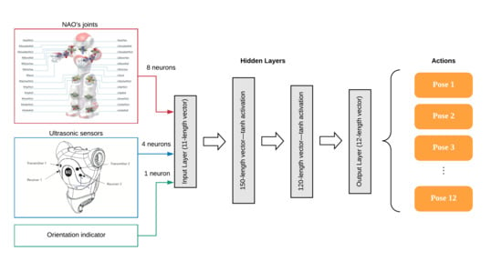
3.3.3. First Level Q-Network
3.3.4. First Level Q-Network Size
3.4. Second Level Module Definition
3.4.1. Actions of the Second Level
3.4.2. State of the Second Level
3.4.3. Reward of the Second Level
3.4.4. Second Level Q-Network
4. Experiment and Results
4.1. Simulation Software
4.2. Q-Network Algorithm
4.2.1. Programming Environment
4.2.2. Fall Module
4.2.3. Algorithm Description
4.3. Learning the Poses
| Left Arm | Right Arm | ||
| L Shoulder Pitch | 105.20 | R Shoulder Pitch | 105.08 |
| L Shoulder Roll | 15.69 | R Shoulder Roll | −15.31 |
| L Elbow Yaw | −85.87 | R Elbow Yaw | 85.85 |
| L Elbow Roll | −29.59 | R Elbow Roll | 29.72 |
| L Wrist Yaw | 0.00 | R Wrist Yaw | 0.00 |
| Left Leg | Right Leg | ||
| L Hip Yaw Pitch | 0.00 | R Hip Yaw Pitch | 0.00 |
| L Hip Roll | 2.87 | R Hip Roll | 2.87 |
| L Hip Pitch | −18.51 | R Hip Pitch | −18.51 |
| L Knee Pitch | 48.04 | R Knee Pitch | 48.04 |
| L Ankle Pitch | −29.53 | R Ankle Pitch | −29.53 |
| L Ankle Roll | −6.33 | R Ankle Roll | −6.33 |
4.4. Learning to Walk
4.4.1. Results for an Action Time of 0.1 s
4.4.2. Results with an Action Time of 0.15 s
4.4.3. Testing with an Action Time of 0.2 s
4.4.4. Testing with an Action Time of 0.25 s
4.4.5. Comparing Results
5. Conclusions and Future Work
5.1. Stability and Not Falling Down
5.2. Actions, States, and Rewards Applicable to Other Robots
5.3. Learning Framework
5.4. Future Work
Supplementary Materials
Author Contributions
Funding
Conflicts of Interest
References
- Shirashaka, S.; Machida, T.; Igarashi, H. Leg Selectable Interface for Walking Robots on Irregular Terrain. In Proceedings of the 2006 SICE-ICASE International Joint Conference, Busan, Korea, 18–21 October 2006. [Google Scholar]
- Ill-Woo, P.; Jung-Yup, K.; Jungho, L. Online Free Walking Trajectory Generation for Biped. In Proceedings of the IEEE Internactional Conference on Robotics and Automation (ICRA 2006), Orlando, FL, USA, 15–19 May 2006; pp. 1231–1236. [Google Scholar]
- Huang, Q.; Kajita, S.; Koyachi, N.; Kaneko, K.; Yokoi, K.; Kotoku, T.; Arai, H.; Komoriya, K.; Tanie, K. Walking patterns and actuator specifications for a biped robot. In Proceedings of the 1999 IEEE/RSJ International Conference on Intelligent Robots and Systems. Human and Environment Friendly Robots with High Intelligence and Emotional Quotients (Cat. No.99CH36289), Kyongju, Korea, 17–21 October 1999. [Google Scholar]
- Tay, A.B. Walking Nao Omnidirectional Bipedal Locomotion. Bachelor’s Thesis, Bachelor of Science, School of Computer Science and Engineering, The University of New South Wales, Kensington, UK, 2009; pp. 1–49. [Google Scholar]
- Morimoto, J.; Cheng, G.; Atkeson, C.G.; Zeglin, G. A simple reinforcement learning algorithm for biped walking. In Proceedings of the IEEE International Conference on Robotics and Automation, 2004. Proceedings. ICRA ‘04. 2004, New Orleans, LA, USA, 26 April–1 May 2004. [Google Scholar]
- Jin-Ling, L.; Kao-Shing, H.; Wei-Cheng, J.; Yu-Jen, C. Gait Balance and Acceleration of a Biped Robot. IEEE Access 2016, 4, 2439–2449. [Google Scholar]
- Michel, O. Webots: Symbiosis between virtual and real mobile robots. In International Conference on Virtual Worlds; Lecture Notes in Computer Science 1434; Springer: Berlin/Heidelberg, Germany, 1998; pp. 254–263. [Google Scholar]
- Hubicki, C.; Abate, A.; Clary, P.; Rezazadeh, S.; Jones, M.; Peekema, A.; Van Why, J.; Domres, R.; Wu, A.; Martin, W.; et al. Walking and running with passive compliance: Lessons from engineering a live demonstration of the ATRIAS biped. IEEE Robot. Autom. Mag. 2018, 25, 23–39. [Google Scholar] [CrossRef]
- Martin, W.C.; Wu, A.; Geyer, H. Robust spring mass model running for a physical bipedal robot. In Proceedings of the 2015 IEEE International Conference on Robotics and Automation (ICRA), Seattle, WA, USA, 26–30 May 2015; pp. 6307–6312. [Google Scholar]
- Hong, S.; Kim, E. A New Automatic Gait Cycle Partitioning Method and Its Application to Human Identification. Int. J. Fuzzy Log. Intell. Syst. 2007, 17, 51–57. [Google Scholar] [CrossRef]
- Jung-Yup, K.; Ill-Woo, P.; Jun-Ho, O. Walking Control Algorithm of Biped Humanoid Robot on Uneven and Inclined Floor. J. Intell. Robot. Syst. 2007, 48, 457–484. [Google Scholar]
- Huang, Q.; Yokoi, K.; Kajita, S.; Kaneko, K.; Arai, H.; Koyachi, N.; Tanie, K. Planning Walking Patterns for a Biped Robot. IEEE Trans. Robot. Autom. 2001, 17, 280–289. [Google Scholar] [CrossRef]
- Lu, Q.; Zheng, Y.; Lu, X. Deviation Correction Control of Biped Robot Walking Path Planning. In IOP Conference Series: Materials Science and Engineering; IOP Publishing: Bristol, UK, 2018; Volume 394, p. 032029. [Google Scholar]
- Ito, S.; Nishio, S.; Ino, M.; Morita, R.; Matsushita, K.; Sasaki, M. Design and adaptive balance control of a biped robot with fewer actuators for slope walking. Mechatronics 2018, 49, 56–66. [Google Scholar] [CrossRef]
- Liu, C.; Yang, J.; An, K.; Chen, Q. Rhythmic-Reflex Hybrid Adaptive Walking Control of Biped Robot. J. Intell. Robot. Syst. 2018, 7, 1–17. [Google Scholar] [CrossRef]
- Righetti, L.; Jan Ijspeert, A. Programmable Central Pattern Generators: An application to biped locomotion control. In Proceedings of the IEEE International Conference on Robotics and Automation, Orlando, FL, USA, 15–19 May 2006; pp. 1585–1590. [Google Scholar]
- Liu, J.; Chen, X.; Veloso, M. Simplified walking: A new way to generate flexible biped patterns. In Mobile Robotics: Solutions and Challenges; World Scientific: Singapore, 2010; pp. 583–590. [Google Scholar]
- Rivas, F.M.; Canas, J.M.; González, J. Automatic learning of walking modes for a humanoid robot (in Spanish). In Proceedings of the Robot2011 III Robotics Workshop, Experimental robotics, Seville, Spain, 28–29 November 2011; pp. 120–127. [Google Scholar]
- Meriçli, Ç.; Veloso, M. Biped walk learning on NAO through playback and real-time corrective demonstration. Workshop on Agents Learning Interactively from Human Teachers. In Proceedings of the 9th International Conference on Autonomous Agents and Multiagent Systems (AAMAS 2010), Toronto, ON, Canada, 9–14 May 2010. [Google Scholar]
- Kao-Shing, H.; Keng-Hao, Y.; Jia-Yan, L. The Study on the Learning of Walking Gaits for Biped Robots. Int. Fed. Autom. Control 2013, 46, 589–593. [Google Scholar]
- Gasparri, G.M.; Manara, S.; Caporale, D.; Averta, G.; Bonilla, M.; Marino, H.; Catalano, M.; Grioli, G.; Bianchi, M.; Bicchi, A.; et al. Efficient Walking Gait Generation via Principal Component Representation of Optimal Trajectories: Application to a Planar Biped Robot with Elastic Joints. IEEE Robot. Autom. Lett. 2018, 3, 2299–2306. [Google Scholar] [CrossRef]
- Corral, E.; Marques, F.; García, M.J.G.; Flores, P.; García-Prada, J.C. Passive walking biped model with dissipative contact and friction forces. In European Conference on Mechanism Science; Springer: Cham, Switzerland, 2019; pp. 35–42. [Google Scholar]
- Dekker, M. Zero-Moment Point Method for Stable Biped Walking; University of Technology: Eindhoven, The Netherlands, 2009. [Google Scholar]
- Strom, J.; Slavov, G.; Chown, E. Omnidirectional Walking Using ZMP and Preview Control for the NAO Humanoid Robot. Lect. Notes Comput. Sci. 2010, 5949, 378–389. [Google Scholar]
- Lee, H.W.; Yang, J.L.; Zhang, S.Q.; Chen, Q. Research on the Stability of Biped Robot Walking on Different Road Surfaces. In Proceedings of the 2018 1st IEEE International Conference on Knowledge Innovation and Invention (ICKII), Jeju, Korea, 23–27 July 2018; pp. 54–57. [Google Scholar]
- Van der Noot, N.; Barrera, A. Zero-Moment Point on a Bipedal Robot. In Proceedings of the 17th IEEE Mediterranean Electrotechnical Conference, Beirut, Lebanon, 13–16 April 2014. [Google Scholar]
- Liu, Y.; Zang, X.; Zhang, N.; Liu, Y.; Wu, M. Effects of unilateral restriction of the metatarsophalangeal joints on biped robot walking. In Proceedings of the 2018 Eighth International Conference on Information Science and Technology (ICIST), Cordoba, Spain, 30 June–6 July 2018; pp. 395–400. [Google Scholar]
- Duysens, J.; Forner-Cordero, A. Walking with perturbations: A guide for biped humans and robots. Bioinspir. Biomim. 2018, 13, 061001. [Google Scholar] [CrossRef] [PubMed]
- Kao-Shing, H.; Jin-Ling, L.; Jhe-Syun, L. Biped Balance Control by Reinforcement Learning. J. Inf. Sci. Eng. 2016, 32, 1041–1060. [Google Scholar]
- McGinnis, P.M. Biomechanics of Sport and Exercise; Human Kinetics Publishers: Champaign, IL, USA, 2015. [Google Scholar]
- Mnih, V.; Kavukcuoglu, K.; Silver, D.; Graves, A. Playing Atari with Deep Reinforcement Learning. arXiv, 2013; arXiv:1312.5602. [Google Scholar]
- Singla, A.; Bhattacharya, S.; Dholakiya, D.; Bhatnagar, S.; Ghosal, A.; Amrutur, B.; Kolathaya, S. Realizing Learned Quadruped Locomotion Behaviors through Kinematic Motion Primitives. arXiv, 2018; arXiv:1810.03842. [Google Scholar]
- Rai, A.; Antonova, R.; Meier, F.; Atkeson, C.G. Using Simulation to Improve Sample-Efficiency of Bayesian Optimization for Bipedal Robots. arXiv, 2018; arXiv:1805.02732. [Google Scholar]
- Michel, O. Webots: Professional Mobile Robot Simulation. Int. J. Adv. Robot. Syst. 2004, 1, 39–42. [Google Scholar] [CrossRef]


| No. | Movement | NAO Joint (in °) | Limit (in °) | ||
|---|---|---|---|---|---|
| From | To | From | To | ||
| 1 | Left shoulder pitch | −119.50 | 119.50 | 70.00 | 110.00 |
| 2 | Left elbow roll | −88.50 | −2.00 | −65.00 | −25.00 |
| 3 | Left, hip pitch | −88.00 | 27.73 | −35.00 | −15.00 |
| 4 | Left knee pitch | −5.29 | 121.04 | 45.00 | 65.00 |
| 5 | Left ankle pitch | −68.15 | 52.86 | −45.00 | −25.00 |
| 6 | Right shoulder pitch | −119.50 | 119.50 | 70.00 | 110.00 |
| 7 | Right elbow roll | −88.50 | −2.00 | −65.00 | −25.00 |
| 8 | Right hip pitch | −88.00 | 27.73 | −35.00 | −15.00 |
| 9 | Right knee pitch | −5.29 | 121.04 | 45.00 | 65.00 |
| 10 | Right ankle pitch | −68.15 | 52.86 | −45.00 | −25.00 |
| Head | |
|---|---|
| Head Pitch | 0 |
| Head Yaw | 0 |
| Q-Network Results | |||||
|---|---|---|---|---|---|
| Action Time | Number of Poses | List of Poses | Distance | Time | Speed |
| 0.10 s | 8 | 10, 1, 3, 4, 7, 7, 8, 12 | 8 cm | 1.621 s | 4.93 cm/s |
| 0.15 s | 5 | 1, 3, 4, 7, 12 | 8 cm | 1.520 s | 5.26 cm/s |
| 0.20 s | 5 | 1, 3, 4, 7, 12 | 8 cm | 2.200 s | 3.63 cm/s |
| 0.25 s | 4 | 1, 4, 7, 12 | 8 cm | 2.015 s | 3.97 cm/s |
| NAO Built-In Walking Controller | |||
|---|---|---|---|
| Mode | Distance | Time | Speed |
| Normal Walking | 8 cm | 2.04 s | 3.92 cm/s |
| Fast Walking | 8 cm | 1.30 s | 6.153 cm/s |
© 2019 by the authors. Licensee MDPI, Basel, Switzerland. This article is an open access article distributed under the terms and conditions of the Creative Commons Attribution (CC BY) license (http://creativecommons.org/licenses/by/4.0/).
Share and Cite
Gil, C.R.; Calvo, H.; Sossa, H. Learning an Efficient Gait Cycle of a Biped Robot Based on Reinforcement Learning and Artificial Neural Networks. Appl. Sci. 2019, 9, 502. https://doi.org/10.3390/app9030502
Gil CR, Calvo H, Sossa H. Learning an Efficient Gait Cycle of a Biped Robot Based on Reinforcement Learning and Artificial Neural Networks. Applied Sciences. 2019; 9(3):502. https://doi.org/10.3390/app9030502
Chicago/Turabian StyleGil, Cristyan R., Hiram Calvo, and Humberto Sossa. 2019. "Learning an Efficient Gait Cycle of a Biped Robot Based on Reinforcement Learning and Artificial Neural Networks" Applied Sciences 9, no. 3: 502. https://doi.org/10.3390/app9030502
APA StyleGil, C. R., Calvo, H., & Sossa, H. (2019). Learning an Efficient Gait Cycle of a Biped Robot Based on Reinforcement Learning and Artificial Neural Networks. Applied Sciences, 9(3), 502. https://doi.org/10.3390/app9030502