Harbor Extraction Based on Edge-Preserve and Edge Categories in High Spatial Resolution Remote-Sensing Images

Abstract

Efficient harbor extraction is essential due to the strategic importance of this target in economic and military construction. However, there are few studies on harbor extraction. In this article, a new harbor extraction algorithm based on edge preservation and edge categories (EC) is proposed for high spatial resolution remote-sensing images. In the preprocessing stage, we propose a local edge preservation algorithm (LEPA) to remove redundant details and reduce useless edges. After acquiring the local edge-preserve images, in order to reduce the redundant matched keypoints and improve the accuracy of the target candidate extraction method, we propose a scale-invariant feature transform (SIFT) keypoints extraction method based on edge categories (EC-SIFT): this method greatly reduces the redundancy of SIFT keypoint and improves the computational complexity of the target extraction system. Finally, the harbor extraction algorithm uses the Support Vector Machine (SVM) classifier to identify the harbor target. The experimental results show that the proposed algorithm effectively removes redundant details and improves the accuracy and efficiency of harbor target extraction.

1. Introduction

With the rapid development of sensor technology, it is easier to obtain high-quality, high spatial resolution remote-sensing images [1]. Therefore, research into using remote-sensing images to extract strategic targets (such as harbors, airports, ships, etc.) becomes very important [2,3,4]. However, existing target recognition algorithms are not suitable for remote-sensing images with complex backgrounds. Therefore, in order to extract regions containing meaningful targets for further processing, this article proposes a new target extraction method based on high spatial resolution remote-sensing images.

A harbor, as an important military and civil constructions, has important practical value for the fields of ship navigation and military reconnaissance, and they are also one of the great focal points for research in the field of pattern recognition and image processing [5,6]. However, there are few studies on harbor target extraction; previous studies on harbor target extraction can be grouped into the following categories: Harbor detection method based on dock (HDD) [7], harbor detection method based on coastline closure (HDC) [8], and harbor detection method based on breakwater (HDB) [9]. We list the advantages and disadvantages of these methods in

Table 1. The advantages and disadvantages of some methods.

Method	Content	Strength	Weakness
HDD [7]	This method is designed according to the characteristic that the harbors have a number of docks that extend to the sea and are pulsed at the junction with the sea.	The detection speed of this method is fast.	It can only extract the docks, so it is impossible to extract the entire harbor targets.
HDC [8]	This method extracts the harbor targets by detecting the semi-closed characteristic of the harbors.	This method can detect artificial/natural harbors, and it has good versatility.	This method has a high rate of false positives: it may mistake a section of the coast without docks for harbors.
HDB [9]	This method is designed according to the characteristic of water surrounding both sides of the harbor breakwaters.	The characteristics of the breakwater are remarkable, and it is easier to extract them.	This method may generate false alarms; it is impossible to extract a complete harbor target.

. Harbor detection method based on dock uses the shape of the dock to determine whether the dock exists. First, this method obtains the feature information of the dock, then the dock candidates are extracted; finally, the dock target is identified by matching the feature points. The disadvantage of this method is that the entire harbor region cannot be accurately identified. Recently, Qi Chen and Junwei Wei have produced valuable research on this method [10,11]. Harbor detection method based on coastline closure uses the characteristics of the strong closure of the harbor target. This method extracts the entire closed regions as harbor targets by establishing a closed region model; it may mistake some natural terrains for harbor targets. Zhu Bing made a detailed study of this method [8]. Harbor detection method based on breakwater uses the characteristics of water surrounding both sides of the harbor breakwaters. First, the breakwater candidates are extracted by edge detection, then the long-striped features of the breakwaters are used to remove the pseudo breakwaters. Finally, the breakwaters of the same harbor are merged by the regional combination method. This method has two problems in the process of extracting the harbor targets: One is that false alarms may occur, and the other is that the extracted harbor targets are breakwaters, so the harbor target regions are incomplete. Chun Liu made a detailed study of this method [9].

In general, previous research extracted harbor targets by detecting docks, breakwaters and closed regions [12]; these methods may lead misidentification and identification of incomplete harbors. A complete harbor target includes its semi-closed geometry, more than two docks and container stacking fields; these features clearly distinguish between harbors and some natural terrains. However, these features are difficult to obtain by traditional image segmentation; moreover, finding them in high-resolution remote-sensing images also requires a lot of calculations.

In order to solve the problems of harbor target extraction, we propose a new harbor extraction algorithm based on edge preservation and a scale-invariant feature transform keypoints extraction method based on edge categories (EC-SIFT) for high spatial resolution remote-sensing images. With the development of the SIFT feature detection algorithm [13], more and more methods based on SIFT are being used in target extraction [14,15]. Therefore, our algorithm uses SIFT to extract the keypoints of harbor targets. In order to improve the efficiency and accuracy of the harbor target extraction, we have improved the process of SIFT keypoints extraction. First, in the preprocessing stage, we proposed a novel local edge-preserve algorithm to remove redundant details and reduce useless edges (such as ships, rocks, buildings, etc.) on the sea and on the ground. Then we proposed EC-SIFT to extract harbor target keypoints; this method greatly reduces the redundancy of SIFT keypoints to further reduce the required calculations. Next, we use the GOM-SIFT algorithm and the QT algorithm to extract harbor candidates. Finally, these harbor candidates are input to the support-vector machine (SVM) to get the harbor target extraction results. The experimental results show that the proposed algorithm reduces the detail redundancy effectively and improves the accuracy and efficiency of harbor target extraction.

The rest of the paper is organized as follows: In Section 2, we introduce the preprocessing method, the LEPA-processing method, and the methods of harbor target candidate extraction. The results of harbor target extraction are shown in Section 3. The discussions of experimental results are provided in Section 4, and the conclusion is provided in Section 5.

2. Materials and Methods

2.1. Pre-Processing and LEPA-Processing

Scale-invariant feature transform feature detection is a very effective method for extracting regions of interest (ROIs) [16,17,18]. A large amount of research on SIFT algorithm is used for extraction of targets, such as airports [19], vehicles [20], and robots [21]. However, the classical SIFT feature detection algorithm is not suitable for extracting the ROIs of remote-sensing images due to the high resolution and complex background [22]. In order to improve the extraction of SIFT keypoints and reduce the computational complexity and interference from complex textures, we use two methods: First, the SIFT detection method usually extracts keypoints in grayscale, so we convert the original image from RGB space to CIE Lab [23]. Then we use the luminance channel L of Lab to extract the SIFT keypoints. Next, image downsampling is used to reduce the number of pixels. I² represents an image which resulted from downsampling the original image I by 2², and we used the original image I(x, y) and the downsampling image I²(x, y) as input images for post-processing.

After preprocessing, the next step is to process the edges of the images. Some previous algorithms mainly do image segmentation based on local information [24], whereas others do some edge smoothing to reduce the detail information [25,26]. However, the former cannot effectively reduce the computational complexity of the feature extraction algorithm, and the latter reduces both useful edge information and useless edge information, which is not the results we hoped for. Therefore, we propose a local edge preservation algorithm (LEPA), which can reduce the edge information of the background and retain the useful edge information. For the harbor target extraction algorithm, we regard small targets (such as ships, rocks, buildings) as backgrounds; reducing their edge information helps us to remove some useless feature points. Next, we introduce this algorithm in detail.

In order to achieve the above objectives, we have improved the image segmentation method. First, we divide the original image R into n sub-regions R₁, R₂, …, R_n. Then we use regional growth method to achieve image segmentation; we set a threshold variable SCOPE when the size of the region R_i is smaller than the threshold SCOPE; we think that region R_i needs to grow, otherwise region R_i stops growing. Finally, we repeat this cycle until the image is split. For the region growth method, we use a function DIFF to achieve the two most similar regions merged; we use a threshold variable MD when the value of the function DIFF is larger than MD, and the size of the region R_i is smaller than SCOPE; it is considered that this region R_i is a small ground target (for example, a small building), so it can be regarded as a background region; we can use the surrounding background region instead of this region because its details are useless. The function DIFF consists of two parts. The first part FD is defined as the difference in characteristics between R_i and R_j, and it is defined as:

$$FD\left(A,B\right)={\displaystyle \sum }_{i=1}^n\parallel {\left(T_i\right)}^A-{\left(T_i\right)}^B\parallel \times W_i$$

(1)

where A, B represent the two image regions, ${\left(T_i\right)}^A$ and ${\left(T_i\right)}^B$ are the feature vector sets of two image regions A and B, respectively, n is the number of selected feature vectors for the region, and W_i is the weight of T.

The second part VAR is defined as the difference in regional variance function, and it is defined as:

$$VAR(A,B)=\parallel va{r}^A-va{r}^B\parallel$$

(2)

Where var^A and var^B are the variance of A and B, respectively.

The reason we add VAR to the DIFF function is that some regions have shadows due to occlusion; this may affect regional segmentation and the determination of small ground targets. For this reason, it is important to use the constraints of variance to increase the reliability of LEPA.

According to the above introduction, the flow of the algorithm is shown in Figure 1.

The specific process of LEPA is as follows:

(I)

We assume that the original image has M × N pixels, we use each pixel as the initial target region R_i, where 0 ≤ i ≤ M × N;

(II)

Set a variable SCOPE to determine if the target region needs to be grown: if the size of R_i is larger than SCOPE, the growth of the R_i is terminated;

(III)

If the size of R_i is smaller than SCOPE, we use the function DIFF to calculate the difference between R_j and every adjacent region R_j.

DIFF(R_i, R_j) = FD(R_i, R_j) × W_FD + VAR(R_i, R_j) × W_VAR

(3)

where W_FD and W_VAR are the weight for FD and VAR, respectively, with 0 ≤ W_FD ≤ 1, 0 ≤ W_VAR ≤ 1, W_FD + W_VAR = 1;

(VI)

Get the smallest DIFF value DIFF_k; for all DIFF_k, we compare the value of DIFF_k and MD. If DIFF_k is larger than MD, R_i is considered a small target, and it will be adjusted to the background region around it. If DIFF_k is smaller than MD, R_i will be merged into the most similar region R_k;

(V)

Perform the above calculations for all regions R_i and then the method continues to the next cycle until all target regions are larger than SCOPE, then the LEPA ends.

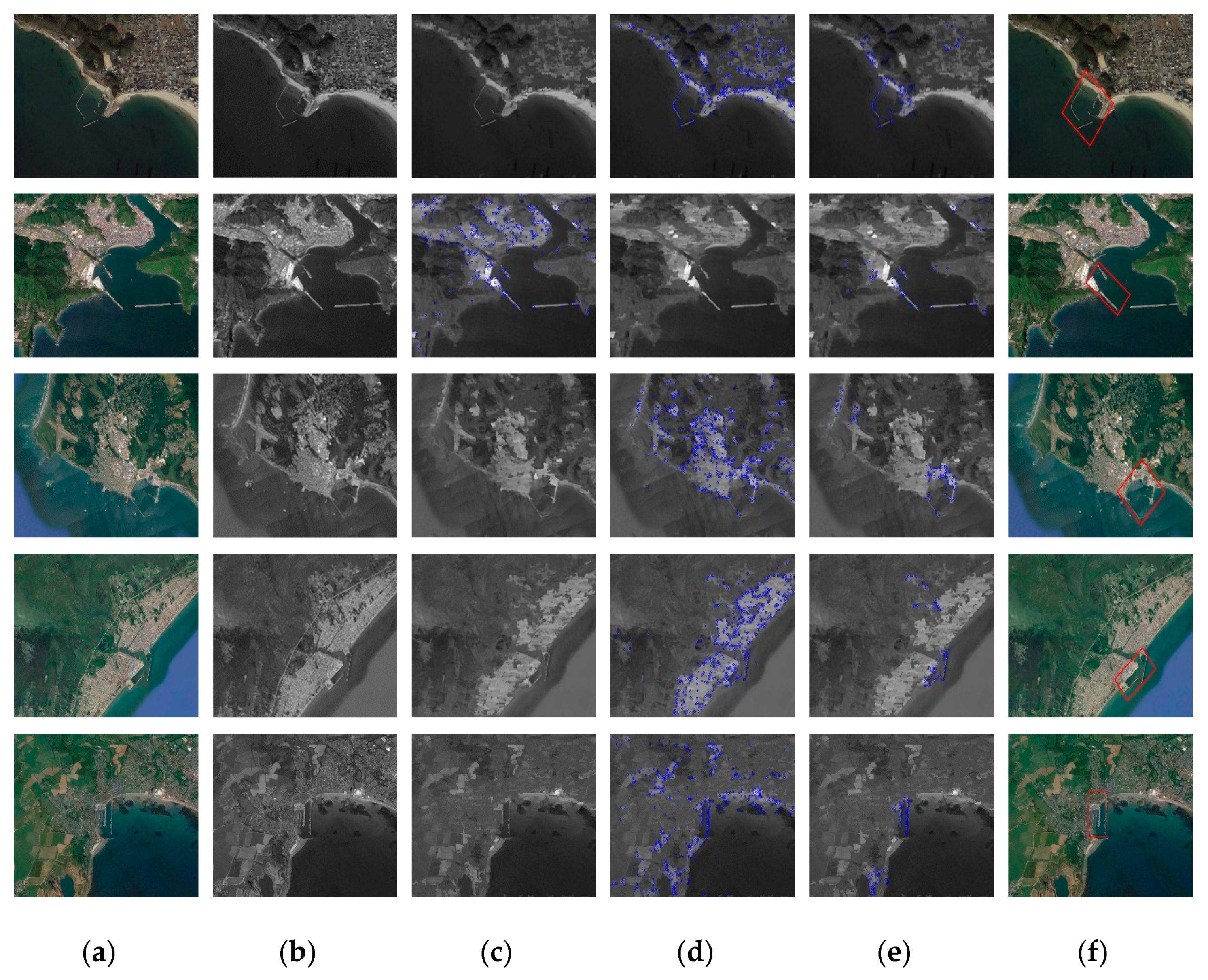
A typical remote-sensing image containing the harbor as a test image of the proposed method, the image processing results and other smoothing algorithms processing results are compared as shown in Figure 2. In this experiment, the value of SCOPE is 150, and the value of MD is 10.

As can be seen, the processing result of our algorithm is better than the general smoothing algorithm and other edge-preserving filtering algorithms. The useless edges in the bilateral filter and guided filter are larger than our method, and the useful edges are less than our method. These results show that our method meets the expected requirements and does not lose too much useful edge information.

2.2. Harbor Candidate Extraction

After image preprocessing, we will extract the candidate regions of the harbors. For a given high-resolution broad-area remote-sensing image, the main characteristics of the harbor are as follows:

(1)

Overall shape of the harbor region is semi-closed and it contains some strip-shaped targets of a certain length (i.e., the jetty, including the breakwater and the code head); the strip-shaped targets are surrounded by water on both sides;

(2)

The gray value of water in the remote-sensing image is generally low and the gray value distribution is uniform (the variance is relatively small), while the gray value and variance of the land are larger than those values of the water, so there is a clear boundary between the water and the land;

(3)

There are more than two jetties in the same harbor, the jetties are adjacent, and two or more jetties are overlapping;

(4)

The container yard around the dock has obvious aspect ratio and has obvious geometric features.

In order to use of the above characteristics of the harbor target and increase the extraction efficiency, we have proposed EC-SIFT, which can remove redundant SIFT keypoints to further reduce the required calculations.

Scale-invariant feature transform is a successful local feature descriptor, which is widely used in template matching of various images. The traditional SIFT algorithm implementation has the following steps: First, extracting SIFT keypoints from the template images and the target images respectively; secondly, describing each SIFT keypoint separately, and it can form a 128-dimensonal keypoint vector for each keypoint; finally, the target extraction results are obtained by matching the keypoint vectors of the target images and the template images. However, when the traditional SIFT algorithm is applied to remote-sensing images, there will be a large number of non-target keypoints; moreover, it is difficult to get all types of harbor templates. Therefore, the keypoints matching for harbor targets may be inaccurate, which directly leads to an increase in the false detection rate of harbor extraction results.

In order to solve these problems, we propose EC-SIFT algorithm to reduce the false detection rate and the number of redundant matching keypoints. The EC-SIFT algorithm combines EC feature and clustering information in the SIFT feature extraction and matching process; we can accurately extract and detect complete harbor candidates. In this part of the article, EC-SIFT algorithm can reduce the redundant keypoints of images. Then, under the guidance of the clustering information, we use the QT algorithm to get the complete harbor candidates. The next section will describe these algorithms in detail.

2.2.1. SIFT Keypoints Extraction Method Based on Edge Categories

The traditional SIFT algorithm takes the extreme points searched in the entire scale space as keypoints, and it will generate a lot of redundant keypoints. Therefore, we propose a keypoint location strategy instead of searching extreme points in the entire scale space. First, we use the geometric invariant moment to extract the EC of images, and then we search for the extreme points corresponding to the EC in the scale space. The flow of the EC-SIFT algorithm is shown in Figure 3.

The EC is defined as a collection of regions containing image edge information, so we look for EC in the image sub-block, and we split the images into image sub-blocks of the same size. In order to make the moment of image sub-blocks have the characteristics of translation, rotation and scale invariance, we use a moment invariant of the Hu moment [27]. It is defined as follows:

Φ(x, y) = η₂₀ + η₀₂

(4)

where x, y are the subscripts of the image sub-blocks.

η_pq represents the normalized center moment; the formula is as follows:

$${\eta }_{pq}=\frac{u_{pq}}{u_{00}^r}\times (r=\frac{q+p}{2})$$

(5)

where u_pq is the central moment, it is defined as follows:

$$u_{pq}={{\displaystyle \sum }}_{x=1}^C{{\displaystyle \sum }}_{y=1}^R{\left(x-x_0\right)}^p\times {\left(y-y_0\right)}^q\times f\left(x,y\right)$$

(6)

x₀, y₀ is the centroid coordinate of the image sub-block region. It is defined as follows:

$$x_0=\frac{m_{10}}{m_{00}},y_0=\frac{m_{01}}{m_{00}}$$

(7)

m_pq is the origin moment, and it is defined as follows:

$$m_{pq}={{\displaystyle \sum }}_{x=1}^C{{\displaystyle \sum }}_{y=1}^R{x}^p\times y^q\times f\left(x,y\right)$$

(8)

The idea of EC extraction is to use image sub-blocks corresponding to local invariant moments whose adjacent moments value jump larger as EC of the images. Therefore, we need to use the moments of adjacent image sub-blocks to calculate the gradient values for the moments of each image sub-block. After the gradient is taken, we set a jump threshold T, and the gradient value of the image sub-block smaller than the threshold T is zeroed; other image sub-blocks are adjusted as EC of the images. The gradient calculation formula of the image sub-block is defined as follows:

$$F\left(x,y\right)=\{\begin{array}{c}G\left(x,y\right)=\left|\Phi \left(x,y\right)-\Phi \left(x+1,y\right)\right|+\left|\Phi \left(x,y\right)-\Phi \left(x,y+1\right)\right|,G\left(x,y\right)\ge T\\ 0,others\end{array}$$

(9)

The local brightness values of the entire image may not be an order of magnitude; thus, if a fixed threshold T is used for all gradient values, a part of the edge regions will be missed when T is too large, and false edge regions will appear when T is too small. We can solve this problem with adaptive threshold T, which is defined as follows:

T = 0.15 × Φ(x, y)

(10)

The above formula determines the threshold T based on the local luminance information, which can distinguish the brightness jumps of different orders of magnitude.

When we segment the image, the image sub-blocks of the edge regions do not all cross the edge line of the image; many image sub-blocks are offset, and some of them even use the image edge lines as the boundary of the image sub-block. If such sub-block is used as the EC region of the image, we will lose a lot of edge information. Therefore, we need to make adjustment to the reserved image sub-blocks, so that the image sub-blocks cross the edge lines as much as possible; in this way, we can ensure that EC contains most of the edge information. We use the adaptive F(x, y) to adjust the starting coordinate of F(x, y) and use the following formula as the condition to terminate the adjustment:

$$|F_{x,y}-\frac{1}{4}(F_{x+1,y}+F_{x-1,y}+F_{x,y+1}+F_{x,y-1})|\le 0.05F_{x,y}$$

(11)

After the above algorithm, we have extracted the EC of images, and the detection of the extreme points will be performed in the corresponding regions of the original images. Figure 4 shows the comparison between keypoints extraction of traditional SIFT algorithm and keypoints extraction of EC-SIFT algorithm in this article. The results show that the EC-SIFT algorithm can improve the traditional SIFT algorithm in two aspects:

(1)

The redundant keypoints are greatly reduced, so that the search speed of SIFT keypoints is increased;

(2)

The search range of the extreme points is reduced, so that the SIFT keypoints are concentrated in the edge regions, which improves the accuracy of the subsequent extraction algorithm.

2.2.2. Harbor Candidate Extraction

After extracting keypoints of SIFT, we will extract harbor candidates. It is a common method to use SIFT keypoints to match template images and target images [28], so we will use this method. Because the breakwaters of harbors are semi-closed and are also prominent in the sea, we use the breakwaters as the main keypoints of matching. First, we use the matching results between the template images and the test image to get the matched keypoints. In the traditional SIFT algorithm, each SIFT keypoint is described by a vector ν=(θ, σ, x, y), where θ is the direction of the feature vector, σ is the scale, x, y are the spatial coordinates of the keypoint. In order to increase the robustness of keypoints matching, we use the gradient orientation modification SIFT (GOM-SIFT) algorithm and the scale restriction criteria algorithm, which are proposed by Z. Yi [29] to improve the matching rate. In this method, we are going to improve the gradient orientations: when the SIFT descriptor samples the image gradient orientations around the keypoints, we found that the grayscale intensities in the same region of some images were completely different, even that the intensity was opposite, so we use GOM-SIFT to modify the gradient direction. The following formula shows the process of modification:

$$\beta \left(\alpha \right)=\{\begin{array}{c}\alpha ,\alpha \in \left[0,180\right]\\ 360-\beta ,\alpha \in \left(180,360\right)\end{array}$$

(12)

where α is gradient orientation and β is modified gradient orientation. However, GOM-SIFT can only remove some incorrect matched keypoints when the image is self-similitude, so we use scale restriction criteria to remove more mismatched keypoints. The definition of scale difference is as follows:

$$SD\left({\upsilon }_1,{\nu }_2\right)={\sigma }_1-{\sigma }_2$$

(13)

We assume that the spatial transformation between pairs of images is affine, and the dimensions of the corresponding local regions are equal, so the SD value of the correct matched pairs should be close to a constant, which means that the SD’s standard deviation of the correct matched pairs should be smaller than the incorrect matched pairs. According to the above principles, we propose scale restriction criteria:

$$a<SD\left({\upsilon }_1,{\nu }_2\right)<b$$

(14)

If a matched pair does not accord with the scale restriction criteria, this matched pair will be rejected. To determine the value of a and b, we form a histogram of all SD values of matched pairs, the peak in the histogram of SD values is recorded as P_SD, and then the values of a and b are obtained by P_SD-W and P_SD+W, respectively, where W is a constant.

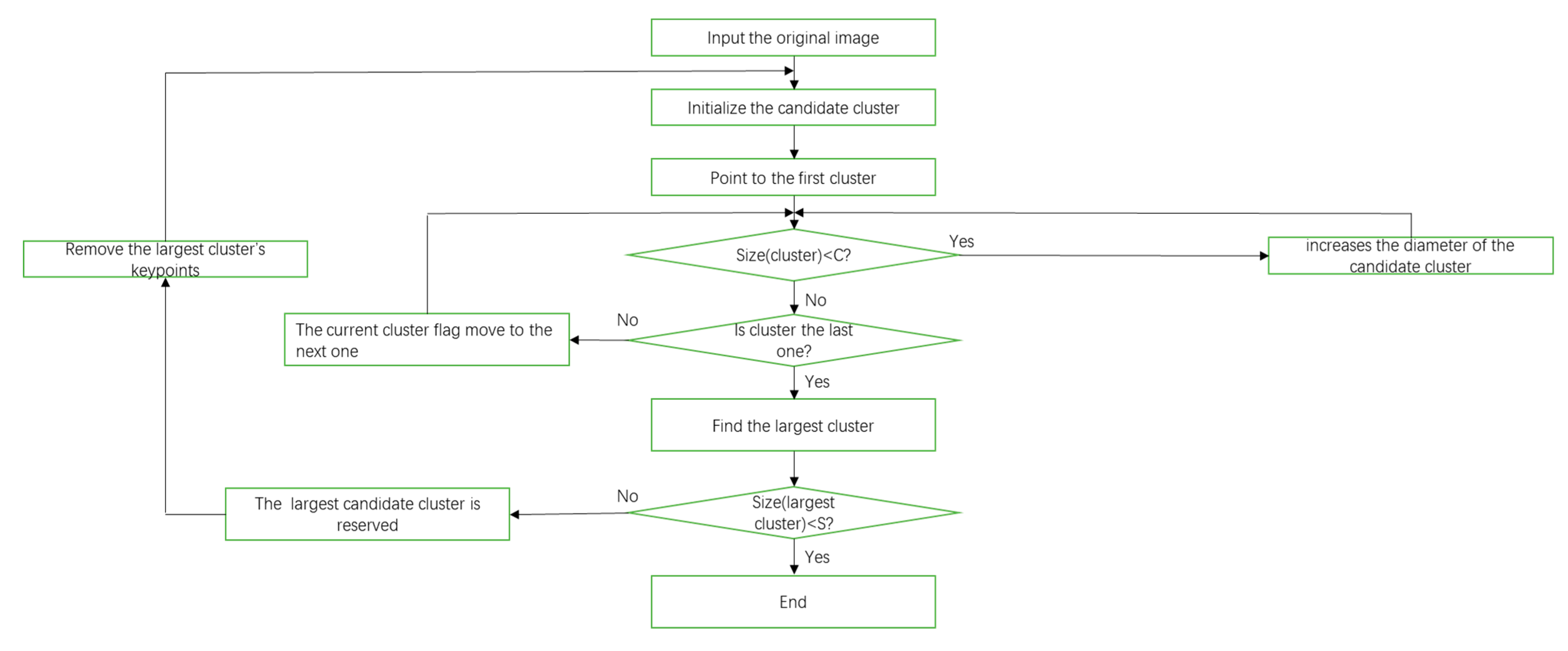
After getting the matched keypoints through GOM-SIFT and scale restriction criteria, we remove some mismatched keypoints. Next, we will use the matched keypoints to extract harbor candidates. Since a harbor is a semi-closed structure, which is composed of regions such as breakwaters and docks, the matched keypoints belonging to the harbor regions should stay within a certain range. Therefore, we get some harbor candidates by dividing the matched keypoints into several groups based on their spatial location. In order to achieve it, we use a quality threshold (QT) clustering method [30], and the flow of the QT algorithm is shown in Figure 5. Quality threshold is an algorithm that classifies matched keypoints into high quality clusters; it ensures high quality clusters by limiting the diameter of the clusters. This method prevents dissimilar keypoints from being forced under the same cluster and ensures that only high-quality clusters are formed. The specific method is implemented as follows:

(1)

Forming a candidate cluster from a single matched keypoint, the growth of the cluster is achieved by adding the matched keypoint around a cluster one by one;

(2)

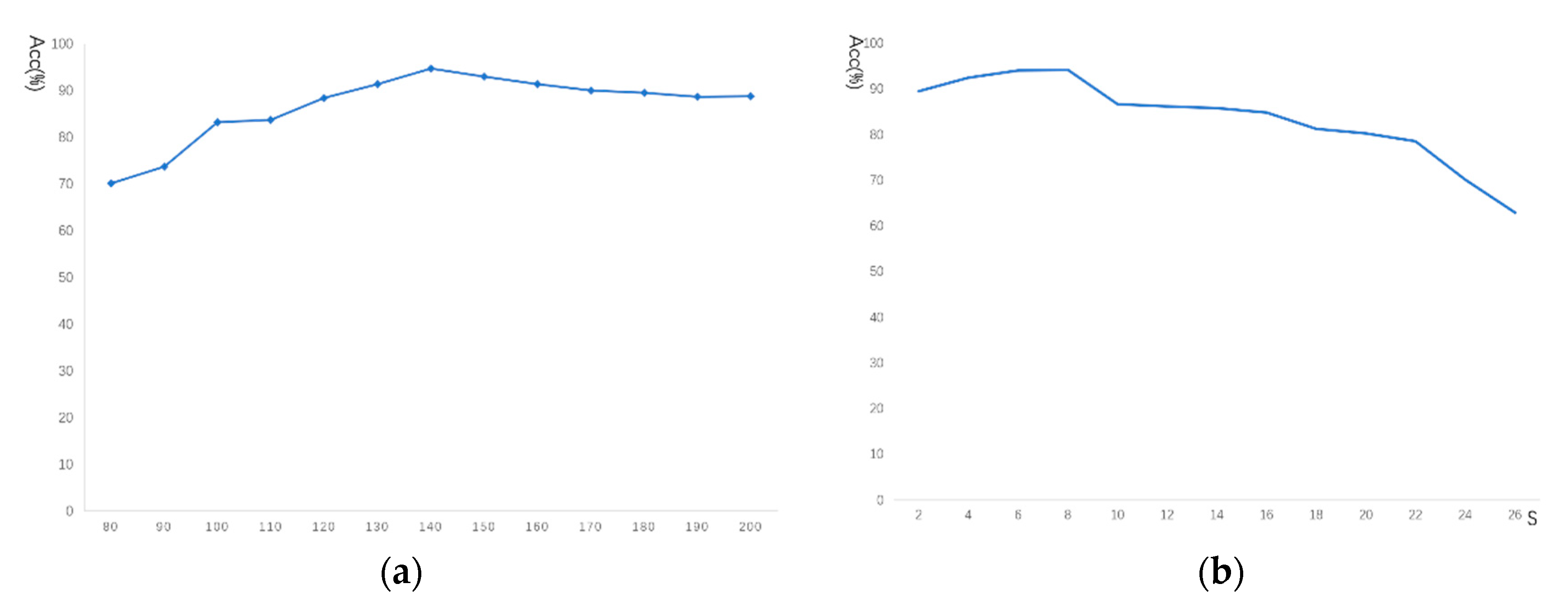
The addition of each associated matched keypoint will increase the diameter of the candidate cluster. We set a maximum diameter threshold C, when the diameter of the cluster exceeds this threshold after increasing the associated matched keypoints, we will stop growing this cluster;

(3)

Subsequent formation of candidate clusters repeats the above process. When forming the candidate clusters, we retain the previous matched keypoints, so we will get the number of candidate clusters with the same number of matched keypoints;

(4)

The largest candidate cluster is reserved, and all the matched keypoints that it contains are removed from the next calculation;

(5)

Repeat the above calculation process;

(6)

Setting a minimum cluster size threshold S. When the diameter of the remaining maximum cluster is smaller than the threshold S, the entire calculation process will stop.

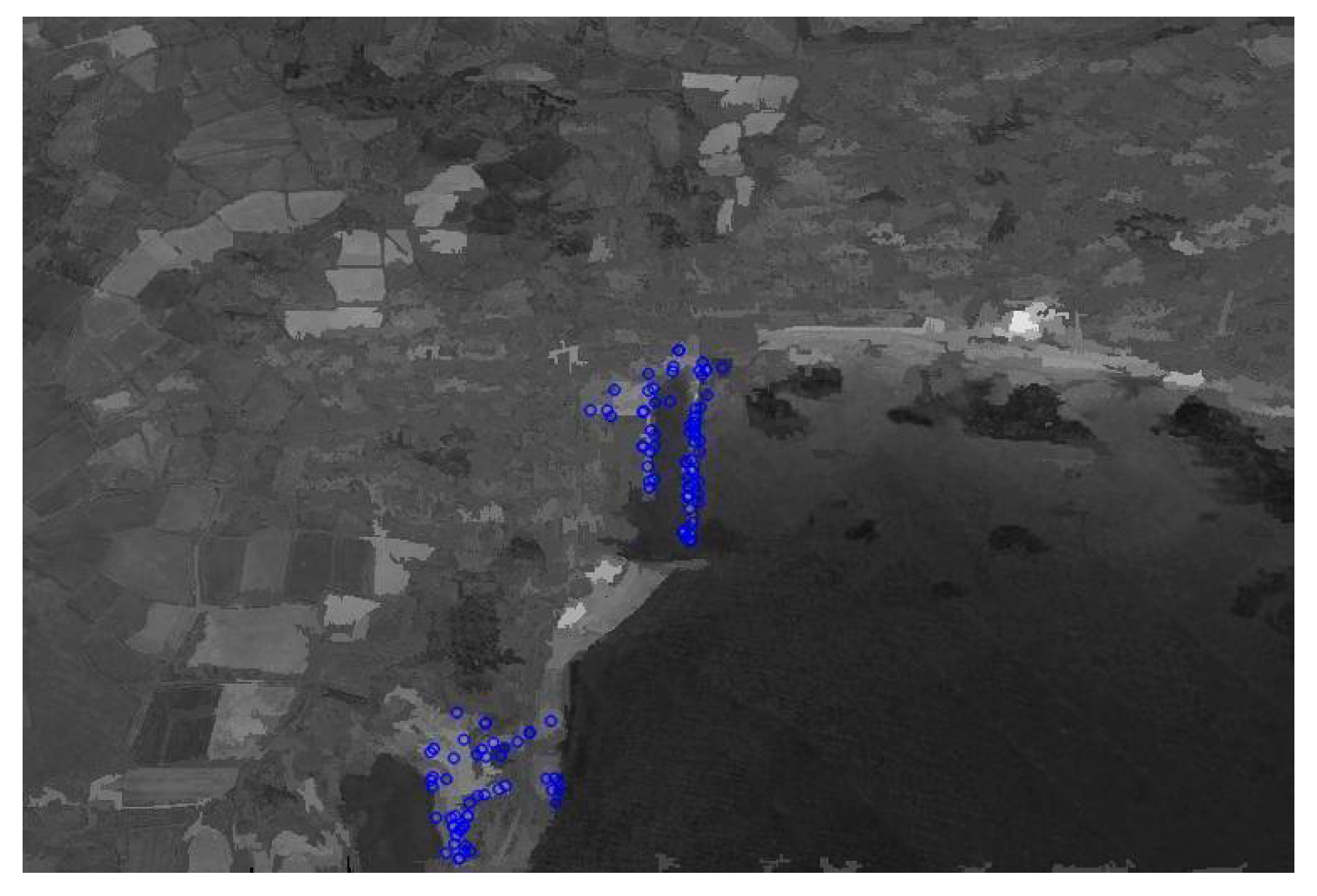
The candidate regions extracted by QT algorithm are shown in Figure 6. These resulting regions are referred to as regions containing the harbor.

3. Results

After getting the harbor candidate regions, we will extract harbor target regions. In this stage, we sort all the harbor candidate regions R_i (i = 1, 2, …, M) according to the number of matched keypoints. For the harbor target extraction process, essentially it is a binary classification process. An SVM is a classical binary classifier, which has many applications in the field of target classification [31] and has many advantages for the application of binary classification detection algorithm, for example, SVM can have good classification results by providing a suitable size dataset. For all of the above reasons, we use the SVM classifier to judge the existence of the harbor region. To build an SVM classifier, we use 3200 images as a training set to train the classifier—1600 images contain harbor (each image contains only one harbor target) and 1600 images do not contain harbor. We adopt remote-sensing images with 756 × 507 pixels from Google Earth and DOTA dataset (the ground-truth harbor regions are also retrieved from this dataset)—all images have the same size and resolution. The features of SVM classifier training are composed of feature vector F = [F₁, F₂, F₃, F₄, F₅, F₆] [32], where F₁ is the mean, F₂ is the standard deviation, F₃ is the mean of the gradient, F₄ is the standard deviation of the gradient, F₅ is the Zernike moment, and F₆ is the circular-Mellin coefficient. Afterward, we use the SVM classifier to identify whether there is a target in these harbor candidate regions. The experimental process and extraction results are shown in Figure 7.

4. Discussion

In this section, we confirmed the validity of the proposed method. For a given high-resolution broad-area remote-sensing image, we use a down sampling method to extract harbor targets in low resolution. The size of the harbor target is a large region, so the size of the harbor candidate region we selected is also a large region. Figure 7 shows the entire experimental process and experimental results; harbor candidate regions containing harbor targets are marked with a red rectangle.

4.1. Result Analysis

The harbor target extraction results we obtained are shown in Figure 7. The test images we selected contain different backgrounds and a variety of harbor targets, and the results show that the proposed algorithm extracts harbor targets very well and successfully removes the pseudo target regions. Then, the quantitative analysis of the proposed method is based on the accuracy of the calculation. The formula for the evaluation is as follows:

$$Acc=\frac{TP+TN}{TP+TN+FP+FN}\times 100\%$$

(15)

where TP denotes the number of true positive harbor targets, TN denotes the number of true negative harbor targets, FP denotes the number of false positive harbor targets, FN denotes the number of false negative harbor targets. Similarly, we use TPR and FPR to evaluate the true positive ratio and the false positive ratio; for the harbor target extraction algorithm, we are pursuing high TPR and low FPR. They are defined as follows:

$$TPR=\frac{TP}{TP+FN}\times 100\%$$

(16)

$$FPR=\frac{FP}{TP+FN}\times 100\%$$

(17)

Other quantitative measurement methods are precision, recall, and F-measure, which are represented by P, R and F_m, respectively. Their definitions are given as follows:

$$P=\frac{TP}{TP+FP}\times 100\%$$

(18)

$$R=\frac{TP}{TP+FN}\times 100\%$$

(19)

$$F_m=\left(1+{\beta }^2\right)\times \frac{P\times R}{{\beta }^2\times P+R}$$

(20)

If the extraction regions contain the complete harbor target, we use the intersection over union (IOU) to evaluate it:

$$IOU=\frac{DR{\displaystyle \cap }GT}{DR{\displaystyle \cap }GT}\times 100\%$$

(21)

where DR denotes Detection Result, GT denotes Ground Truth.

We use 3000 images as test images—1600 images contain harbor and 1400 images do not contain harbor to get the extraction results for the experiment. Harbor targets are correctly extracted in 1527 existing target images (TP = 1527), harbor targets are extracted incorrectly in 84 non-existent images (FP = 84), no harbor targets are extracted in the 73 existing target images (FN = 73), no harbor targets extracted in 1316 non-existent target images (TN = 1316). Therefore, the accuracy of the calculation is 94.77%, the calculation result of IOU is 88.43%, the results of other evaluation functions are shown in Table 3, so our algorithm proves to be effective.

Table 2. Accuracy (Acc), true positive ratio (TPR), false positive ratio (FPR) and intersection over union (IOU) of our method and four competing methods.

Method	Acc(%)	TPR(%)	FPR(%)	IOU(%)
HDD	86.23	88.38	16.21	70.62
HDC	82.07	83.56	19.64	77.96
HDB	77.37	81.44	27.29	74.45
HDM	91.30	91.94	9.43	85.16
Our method	94.77	95.44	6.00	88.43

,

Table 3. Precision, Recall and F-measure of our method and four competing methods.

Method	Precision(%)	Recall(%)	F-measure
HDD	86.17	88.38	0.8726
HDC	82.94	83.56	0.8325
HDB	77.33	81.44	0.7933
HDM	91.77	91.94	0.9185
Our method	94.79	95.44	0.9511

,

Table 4. True positive (TP), false positive (FP), existing target images (FN) and non-existing target images (TN) of our method and four competing methods.

Method	TP	FP	FN	TN
HDD	1414	227	186	1173
HDC	1337	275	263	1125
HDB	1303	382	297	1018
HDM	1471	132	129	1268
Our method	1527	84	73	1316

and Figure 8 show a comparison of our algorithm with some other target extraction algorithms. We have chosen some typical harbor extraction algorithms, such as HDD [7], HDC [8], HDB [9] and HDM [33], and in the calculation of these methods, we used the same test dataset and training dataset as our method. The average processing times of these methods are shown in

Table 5. Average time (s) of four competing methods and our method.

Method	Average Running Time (s)
HDD	11.15
HDC	6.36
HDB	5.14
HDM	24.37
Our method	2.69

. All the experiments are carried out in the Visual Studio 2015 environment with 3.5 Ghz CPU, 16 GB RAM. It can be seen that our algorithm has higher extraction accuracy and lower computational complexity.

Figure 9 shows the receiver operating characteristic (ROC) curve and the Precision–recall curves of our method and four other methods. These two curves are important indicators for evaluating the performance of the harbor target extraction method. We can evaluate the performance of the methods by comparing the area under the curve of these methods: The larger the area under the curve, the better the performance of the method. According to Figure 9a,b, our method performs better than four other methods.

4.2. Analysis of Parameter Selection

In order to select more accurate parameters, we evaluated the performance of the harbor target extraction algorithm under different parameters. First, we determine the values of the SCOPE and MD in the LEPA. We use different SCOPE values to evaluate the effect of SCOPE on the selected image, which is shown in Figure 10. We evaluate the effect of different SCOPE values on the image by calculating the standard deviation of the image and the entropy of the image. Then, in order to explain that the algorithm keeps the useful edge information as much as possible, we calculate the total number of edge pixels of the image and the number of edge pixels in the harbor region. The specific method is as follows:

$$\delta =\sqrt{\frac{1}{M\times N}{\displaystyle \sum }_{i=1}^M{\displaystyle \sum }_{j=1}^N{\left(f\left(i,j\right)-\mu \right)}^2}$$

(22)

The above formula is the standard deviation calculation of the image: M, N represents the size of the image, f(i, j) is the pixel value at the coordinate (i, j), and μ is the average value of the image. This formula reflects the degree of dispersion between the individual pixel value and the mean value of the image. In this experiment, we hope that the standard deviation of the image to be as small as possible, which means that there are fewer details in the image.

We use two-dimensional entropy as another evaluation function, and the specific formula is as follows:

$$P_{ij}=c\left(m,n\right)/D^2$$

(23)

$$H={\displaystyle \sum }_{m=0}^{255}{P}_{mn}log{P}_{mn}$$

(24)

where m is the gray value of the pixel, n is the mean value of the neighborhood gray, c(m, n) is the frequency of the binary group(m, n), D is the scale of the image, and the default value of D is 9. In this experiment, we hope that the value of entropy will be as small as possible, which means that the details of the image are small.

Then we count the total number of edge pixels in the image and the number of edge pixels in the harbor region, which are summarized in

Table 6. The values of standard deviation, entropy, available edge pixels and edge pixels corresponding to the values of different parameter SCOPE.

SCOPE	Available Edge Pixels	Edge Pixels	Standard Deviation	Entropy
100	6763	93,328	26.7462	6.4968
110	6727	87,341	26.4216	6.4758
120	6658	79,495	25.6472	6.4137
130	6562	70,542	24.5879	6.3843
140	6430	61,587	23.0124	6.2648
150	6217	51,569	21.6932	6.1786
160	5794	44,325	21.0219	6.1125
170	4623	38,224	20.6348	6.0644
180	3976	34,156	20.2591	6.0031
190	3477	33,269	20.1446	5.9412
200	3025	32,596	20.0536	5.8903

to illustrate the reliability of the parameters that we selected. The number of pixels in the image is 383,292, and the number of pixels in the harbor region is 7480.

Using the above data, we have drawn the graphs shown in Figure 11. According to the comparison of these evaluation data, we should make sure that the available edge pixels are enough, and the standard deviation and the entropy should be as small as possible; therefore, the value of SCOPE equal to 150 is selected.

For the selection of the parameter MD, we use different MD values to evaluate the effect of MD on the selected image, which is shown in Figure 10. The evaluation method is the same as that of SCOPE; we use standard deviation, entropy, available edge pixels and edge pixels to evaluate the effect of different MD values on the image. The experimental results are shown in Figure 12 and

Table 7. The values of standard deviation, entropy, available edge pixels and edge pixels corresponding to the values of different parameter MD.

MD	Available Edge Pixels	Edge Pixels	Standard Deviation	Entropy
5	6619	91,135	26.4143	6.2712
6	6592	86,544	26.2855	6.2457
7	6471	76,686	25.4572	6.1962
8	6419	67,871	24.2884	6.1338
9	6326	59,462	22.7393	6.0476
10	6187	48,750	21.4425	5.9448
11	5964	41,338	20.8777	5.8261
12	4688	34,947	20.4661	5.7443
13	4283	32,276	20.1287	5.6981
14	3954	30,841	19.9776	5.6570
15	3748	29,488	19.9343	5.6325

.

According to the comparison of these evaluation data, we should make sure that the number of available edge pixels are enough, and the standard deviation and the entropy should be as small as possible; therefore, the value of MD equal to 10 is selected.

In order to determine the parameters C and S, we choose Acc as an indicator to evaluate the quality of parameters. Figure 13 shows the effect of the selection of different C, S values on the final extraction accuracy.

From Figure 13a, it can be seen that, when parameter C = 140, the value of Acc reaches the maximum value, and as the value of C continues to increase, the Acc decreases slightly. From Figure 13b, we can see that the value of Acc decreases as the parameter S increases. However, when the value of S is too small, the computational complexity will increase. Therefore, the value of S in this experiment is chosen to be 8 by considering things comprehensively.

5. Conclusions

In this article, we proposed a novel harbor extraction algorithm for high spatial resolution remote-sensing images, which is based on LEPA and EC-SIFT algorithms. First, in order to reduce the detail information of complex background for high spatial resolution remote-sensing images, we proposed a LEPA algorithm, which effectively reduces the interference of redundant detail information in the extraction algorithm and also retains useful feature information. Then we used the EC-SIFT algorithm to limit the extraction of keypoints to the edge regions, which makes our calculations in the process of keypoints matching and target extraction more accurate and less computational complexity. Finally, we used GOM-SIFT algorithm and QT clustering algorithm to extract the harbor candidate regions, and the SVM was used to identify the region containing the harbor target. In the experiment, we used 3000 test images and classical evaluation functions to evaluate the proposed harbor extraction algorithm. The results show that our algorithm has a significant effect in improving extraction accuracy and reducing computational complexity. It also outperforms other traditional harbor extraction algorithms. The proposed algorithm can be extended to other man-made target extraction in high spatial resolution remote-sensing images, such as airports and military bases, which requires additional research.

References

1. Jin, L.; Liu, Z.; Liu, F. Compressive sampling based on frequency saliency for remote sensing imaging. Sci. Rep. 2017, 7, 6539. [Google Scholar]
2. Zhao, Q.-P.; Yao, L.-X.; He, H.-Y.; Yang, J. Target Extraction Method Based on Region of Interest; Institute of Image Processing and Pattern Recognition; Shanghai Jiaotong University: Shanghai, China, 2006. [Google Scholar]
3. Fu, K.; Li, Y.; Sun, H.; Yang, X.; Xu, G.; Li, Y.; Sun, X. A Ship Rotation Detection Model in Remote Sensing Images Based on Feature Fusion Pyramid Network and Deep Reinforcement Learning. Remote Sens. 2018, 10, 1922. [Google Scholar] [CrossRef]
4. Bentes, C.; Velotto, D.; Tings, B. Ship Classification in TerraSAR-X Images with Convolutional Neural Networks. IEEE J. Ocean. Eng. 2017, PP, 1–9. [Google Scholar] [CrossRef]
5. Yongjie, H.; Wang, S.; Xing, K. Recognition method of harbor target in remote sensing image. In Proceedings of the International Symposium on Multispectral Image Processing & Pattern Recognition International Society for Optics and Photonics, Xiangyang, China, 28–29 October 2007. [Google Scholar]
6. Liu, C.; Yin, J.J.; Yang, J. Target recognition method for T-Shaped harbor in polarimetric SAR images. Chin. J. Radio Sci. 2016, 1, 19–24. [Google Scholar]
7. Mandal, D.P.; Murthy, C.A.; Pal, S.K. Analysis of IRS Imagery for Detecting Man-Made Objects with a Multivalued Recognition System. IEEE Trans. Syst. Man Cybern. Part A Syst. Humans. 1996, 26, 241–247. [Google Scholar] [CrossRef]
8. Zhu, B.; Li, J.; Cheng, A. Knowledge based recognition of harbor target. J. Syst. Eng. Electron. 2006, 17, 755–759. [Google Scholar]
9. Chun, L. Harbor Detection in Polarimetric SAR Images Based on the Characteristics of Parallel Curves. IEEE Geosci. Remote Sens. Lett. 2016, 13, 1400–1404. [Google Scholar]
10. Qi, C. Harbor Detection of Remote Sensing Images Based on Model. Signal Process. 2010, 1, V1-322–V1-325. [Google Scholar]
11. Wei, J.W. Research and Implement of Harbor Detection in Remote; Xidian University: Xi’an, China, 2007. [Google Scholar]
12. Qi, C. Harbor Detection Method of SAR Remote Sensing Images Based on Feature. J. Electron. Inf. Technol. 2010, 32, 2873–2878. [Google Scholar]
13. Lowe, D.G. Distinctive Image Features from Scale-Invariant Keypoints. Int. J. Comput. Vis. 2004, 60, 91–110. [Google Scholar] [CrossRef] [Green Version]
14. Johnson, A.E.; Hebert, M. Recognizing Objects by Matching Oriented Points. In Proceedings of the IEEE Computer Society Conference on Computer Vision & Pattern Recognition, San Juan, PR, USA, 17–19 June 1997. [Google Scholar]
15. Ferrari, V.; Tuytelaars, T.; Gool, L.V. Simultaneous Object Recognition and Segmentation from Single or Multiple Model Views. Int. J. Comput. Vis. 2006, 67, 159–188. [Google Scholar] [CrossRef] [Green Version]
16. Agrawal, A.; Mangalraj, P.; Mukul, A.B. Target detection in SAR images using SIFT. In Proceedings of the IEEE International Symposium on Signal Processing & Information Technology, Abu Dhabi, UAE, 7–10 December 2015. [Google Scholar]
17. Deyun, Z.; Lina, Z.; Kun, Z. A Novel SAR Target Detection Algorithm via Multi-Scale SIFT Features. J. Northwest. Polytech. Univ. 2015, 33, 867–873. [Google Scholar]
18. He, L.; Yang, J.; Kong, B.; Wang, C. An Automatic Measurement Method for Absolute Depth of Objects in Two Monocular Images Based on SIFT Feature. Appl. Sci. 2017, 7, 517. [Google Scholar] [CrossRef]
19. Zhu, D.; Wang, B.; Zhang, L. Airport Target Detection in Remote Sensing Images: A New Method Based on Two-Way Saliency. IEEE Geosci. Remote Sens. Lett. 2015, 12, 1096–1100. [Google Scholar]
20. Zhang, C.; Wang, X.; Feng, J.; Cheng, Y. SiftKeyPre: A Vehicle Recognition Method Based on SIFT Key-Points Preference in Car-Face Image. Computer Vision. In Proceedings of the CCCV 2015 Communications in Computer and Information Science, Xi’an, China, 18–20 September 2015; Springer: Berlin/Heidelberg, Germany, 2015; Volume 547. [Google Scholar]
21. Du, Y.H. SIFT-Based Target Recognition in Robot Soccer. Key Eng. Mater. 2016, 9, 693. [Google Scholar] [CrossRef]
22. Sirmacek, B.; Unsalan, C. Urban-Area and Building Detection Using SIFT Keypoints and Graph Theory. IEEE Trans. Geosci. Remote Sens. 2009, 47, 1156–1167. [Google Scholar] [CrossRef]
23. Xiaomin, P.; Zijian, M.; Jiangming, K. Color image segmentation based on HSI and LAB color space. J. Guangxi Univ. 2011, 36, 976–980. [Google Scholar]
24. Benz, U.C. Multi-resolution, object-oriented fuzzy analysis of remote sensing data for GIS-ready information. ISPRS J. Photogramm. Remote Sens. 2011, 58, 239–258. [Google Scholar] [CrossRef]
25. Arce, R.G. Multistage order statistic filters for image sequence processing. IEEE Trans. Signal Process. 1991, 39, 1146–1163. [Google Scholar] [CrossRef]
26. Tekalp, M.A. Digital Video Processing; Tsinghua University Press: Beijing, China, 1998. [Google Scholar]
27. Mingkuei, H. Visual pattern recognition by moment invariants. IRE Trans. Inf. Theory 1962, 8, 179–187. [Google Scholar] [CrossRef]
28. Karine, A.; Toumi, A.; Khenchaf, A.; El Hassouni, M. Radar Target Recognition Using Salient Keypoint Descriptors and Multitask Sparse Representation. Remote Sens. 2018, 10, 843. [Google Scholar] [CrossRef]
29. Yi, Z.; Cao, Z.; Yang, X. Multi-spectral remote image registration based on SIFT. Electron. Lett. 2008, 44, 107–108. [Google Scholar] [CrossRef]
30. Heyer, L.J.; Kruglyak, S.; Yooseph, S. Exploring Expression Data: Identification and Analysis of Coexpressed Genes. Genome Res. 1999, 9, 1106. [Google Scholar] [CrossRef] [PubMed]
31. Zhu, Q.; Zhong, Y.; Zhao, B.; Xia, G.; Zhang, L. The bag-of-visual-words scene classifier combining local and global features for high spatial resolution imagery. In Proceedings of the International Conference on Fuzzy Systems & Knowledge Discovery, Zhangjiajie, China, 15–17 August 2016. [Google Scholar]
32. Liu, D.; He, L.; Carin, L. Airport detection in large aerial optical imagery. In Proceedings of the 2004 IEEE International Conference on Acoustics, Speech, and Signal Processing, Montreal, QC, Canada, 17–21 May 2004. [Google Scholar]
33. Li, Y.; Peng, J. Feature extraction and recognition of harbor contour. Proc. SPIE 2001, 4550, 234–238. [Google Scholar]
Figure 1. Flow chart for local edge preservation algorithm (LEPA).
Applsci 09 00420 g001
Figure 2. (a) The original image. (b) The edge detection result of original image by Prewitt. (c) The smoothing result by the bilateral filtering algorithm. (d) The edge detection result of Figure 2c by Prewitt. (e) The smoothing result by the general edge-preserve algorithm. (f) The edge detection result of Figure 2e by Prewitt. (g) The smoothing result by the guided filtering algorithm. (h) The edge detection result of Figure 2g by Prewitt. (i) The smoothing result by the method proposed. (j) The edge detection result of Figure 2i by Prewitt.
Applsci 09 00420 g002aApplsci 09 00420 g002b
Figure 3. Flow chart for a scale-invariant feature transform keypoints extraction method based on edge categories (EC-SIFT) algorithm.
Applsci 09 00420 g003
Figure 4. (a) Original image. (b) Traditional scale-invariant feature transform (SIFT) keypoints extraction. (c) Original image. (d) EC-SIFT keypoints extraction.
Applsci 09 00420 g004
Figure 5. Flow chart for quality threshold (QT) algorithm.
Applsci 09 00420 g005
Figure 6. Improved harbor candidate region extraction result.
Applsci 09 00420 g006
Figure 7. (a) Original image. (b) Extracting image luminance channel. (c) Processing results of LEPA algorithm. (d) Processing results of EC-SIFT algorithm. (e) Harbor candidate region extraction results. (f) Harbor target extraction results.
Applsci 09 00420 g007
Figure 8. (a) Original image. (b) Harbor extraction result based on dock. (c) Harbor detection result based on coastline closure. (d) Harbor detection result based on breakwater. (e) Harbor detection result based on model matching. (f) Harbor target detection result based on our method.
Applsci 09 00420 g008
Figure 9. (a) Receiver operating characteristic (ROC) curves of our method and four competing methods with different colors that represent different methods. (b) Precision–recall curves of our method and four competing methods with different colors that represent different methods.
Applsci 09 00420 g009
Figure 10. Selected image.
Applsci 09 00420 g010
Figure 11. (a) The number of available edge pixels corresponding to the values of different parameter SCOPE. (b) The number of edge pixels corresponding to the values of different parameter SCOPE. (c) The values of standard deviation corresponding to the values of different parameter SCOPE. (d) The values of entropy corresponding to the values of different parameter SCOPE.
Applsci 09 00420 g011
Figure 12. (a) The number of available edge pixels corresponding to the values of different parameter MD. (b) The number of edge pixels corresponding to the values of different parameter MD. (c) The values of standard deviation corresponding to the values of different parameter MD. (d) The values of entropy corresponding to the values of different parameter MD.
Applsci 09 00420 g012
Figure 13. (a) The values of Acc corresponding to the values of different parameter C. (b) The values of Acc corresponding to the values of different parameter S.
Applsci 09 00420 g013