1. Introduction
The strandbeest elegantly manifested a bio-inspired locomotion by means of mechanism was introduced by Theo Jansen in 1990 [
1]. The innovative mechanism to implement legged motion is called a Theo Jansen Linkage (TJL), which consisted of eight links. Once the ensemble of its links is determined, it can generate a deterministic orbit. The oval orbit produced by the TJL, possessing a transversal axis longer than a lateral axis, achieves energy efficient walking as comparing to the circular orbit that is generated by the four-bar linkage [
2].
It soon drew attention from some robotics researchers. In the attempt of achieving motions, such as climbing or skipping, other than walking, Komoda [
3] changed a static point of a TJL to be movable and studied its singularity [
4]. Mohsenizadeh [
5] employed the loop closure equations method to analyze the kinematics of TJLs and validated it with the simulation in SolidWorks. Nansai [
6] employed the projection method, a technique dealing with constraint forces to analyze the dynamics of TJLs. Later on, he also investigated the position and velocity control of TJLs [
7,
8]. So far, all of academic works that are relevant to TJLs focus on the analysis of kinematics, dynamics, and controls. None has ever addressed the issue of design. It is of interest to note that the analysis is mainly to study the forward problems while the design has to rely on the knowledge of inverse problems. For instance, the kinematics of the TJL can be derived according to the Denavit–Hartenberg convention along with some trigonometric constraints. It well defines a forward problem, i.e., given the dimension of the TJL to generate the orbit. Nevertheless, how to design a TJL to achieve locomotion is in fact a sort of inverse problems, i.e., given a specification of orbit to determine the dimension of the TJL.
The primary goal of this paper is to develop a technique to design the TJLs, i.e., solving its inverse problem. Conventionally, the standard numerical scheme called LM (Levenberg–Marquardt) method [
9,
10] is an effective tool to solve the inverse problems. However, the patterns of orbits produced by the TJL may vary according to its ensemble dimension and can be casted into four groups, such as bell curves, ovals, sharp-pointed ovals, and lemniscates. Some orbits can be used as the foot trajectories for legged robots but some cannot. Overall speaking, the ovals or bell orbits are legitimate and the sharp-pointed ovals are partly legitimate, nevertheless the lemniscates are illegitimate. Although the algorithm of LM always leads to a (locally optimal) solution, it does not guarantee the solution falling into the legitimate class because it is unable to tell the patterns of orbits.
Besides, the way of given a prescribed orbit to determine the dimension of a TJL is too strict to be practical. The pattern of foot trajectories is only one factor in designing a legged robot. In general, it demands abundant feasible designs in which a designer can make a trade off when other factors are taken into account. Hence, it is vital to give a guideline, to which one can refer, to ensure that the design of a TJL always possesses its eligibility that is generating a legitimate orbit for a legged robot. In the attempt of gathering feasible designs to establish a database, difficulty arises as to how to distinguish the feasible data from the infeasible ones among a vast amount of data. We propose employing the ML (Machine Learning) technique [
11,
12,
13] called SVM (Support Vector Machine) along with machine vision [
14,
15] to tackle this problem. There are two merits of using SVM. First, it gives a geometric perspective that is finding the equation for a hyperplane to best separate the different classes in the feature space. Second, it solves the convex optimization problem analytically and hence always returns the same optimal hyperplane.
The proposed method is divided into two steps. First, a preliminary model is built with a small portion of data to conduct a pilot study on discovering the knowledge of data. Second, an advanced model is built to deal with large scale data and to fulfill the inverse problem.
In the preliminary model, the training data will be classified by our human vision and based upon intuitive judgement that the major axis of an orbit is closely aligned with the horizontal and the shape of an orbit possessing no self-intersection should be neither too slim nor too thick. Subsequently, the image processing is applied to extract two properties from the image of each orbit, i.e., obliqueness and slenderness . When remapping the training data under these two properties, it unveils that the legitimate data tend to cluster within a region that is consistent with our preference in classification. It means that both obliqueness and slenderness are sufficient to characterize the orbits, based upon which our vague preference can be turned into definite mathematical criteria and the machine vision can be applied to label the orbits.
In the advanced model, two SVMs are trained and two databases concerned with properties and dimensions of all eligible designs are established. The models of SVM are used to quickly identify the eligibility of a design and the databases provide abundant of feasible data to which a designer can refer as designing the TJLs. Moreover, a program can be developed to fulfill the inverse problem. It searches the orbits in compliance with the specification of and from the database of properties and uses their correspondent identity numbers to list all candidates of TJLs from the database of dimensions.
2. Theo Jansen Linkage and Foot Trajectories
The TJL can be built either using eight links or twelve links. It depends on the way of fabricating two triangluar links of the TJL. If each triangular link is machined into a whole piece, then the TLJ is an eight-bar linkage. If each of them is assembled by three straight bars, the TLJ will be a twelve-bar linkage. Regardless of eight or twelve, the degrees of freedom of the TJLs turn out to be the same, i.e., one. The TJL in this paper is the eight-bar linkage, as shown in
Figure 1a, where the TJL is normalized with respect to its link-1, so that link-1, 2, 3, 6, 7 are straight bars with lengths 1, a, b, d, d, respectively; link-4, 5 are isosceles right triangles with sides of length c; link-8 is a rectangular fixture with dimensions S
x and S
y. In
Figure 1b, a robot is mounted with TJLs to achieve the legged motion.
The kinematics of the TJL can be derived according to the Denavit-Hartenberg [
16,
17] convention along with some trigonometric constraints. Hence, the foot trajectory at the point E is a function of the input variable
defined, as follows.
where
With the aid of kinematic Equations (1)–(11), the orbit of a TJL can be determined provided that the six parameters, i.e., a, b, c, d, Sx, Sy, are given. This is so called the forward problem. However, designing a TJL to generate a legitimate orbit is an inverse problem, i.e., given the specification of an orbit to determine six parameters, a, b, c, d, Sx, Sy. It is hopeless to derive any analytical function to deal with this inverse problem. Hence, the numerical schemes have to be applied.
The LM (Levenberg–Marquardt) method [
9,
10] is a standard numerical scheme in solving the inverse problems. Supposedly, the six unknown parameters can be obtained by minimizing an objective function, which is the square of residual between the desired and actual orbits. However, let us take a glimpse of
Figure 2, where the orbits are generated by randomly resizing TJLs. The patterns of orbits can be roughly casted into four patterns, i.e., bell curves, ovals, sharp-pointed ovals, and lemniscates, as shown in
Figure 3.
Some orbits, named as legitimate class, can be used as the foot trajectories for legged robots, but some, named as illegitimate class, cannot. Overall speaking, the ovals or bell orbits are legitimate and the sharp-pointed ovals are partly legitimate, nevertheless the lemniscates are illegitimate. Unfortunately, the LM method is unable to tell the patterns of orbits. Hence, its algorithm does not guarantee that its solution always stays within the legitimate class. In other words, the LM method is a numerical scheme good for the case of homogeneity, i.e., all orbits belonging to the legitimate class. As encountered with the case of heterogeneity, i.e., legitimate orbits mingled with illegitimate ones, it becomes so incompetent.
Since neither the analytical method nor the standard numerical scheme can prevail, we resort to leverage the ML (Machine Learning) in the attempt of drawing out the knowledge or model from those heterogeneous data, i.e., orbits. Many different types of ML techniques have been developed and they can be categorized into three types, i.e., supervised learning, unsupervised learning, and reinforcement learning, depending on the training method. Among them, a supervised learning technique, called SVM, will be employed here to achieve the binary classification. There are two merits of using SVM. First, it gives a geometric perspective that is finding the equation for a hyperplane to best separate the different classes in the feature space. Second, it solves the convex optimization problem analytically and hence always returns the same optimal hyperplane. Due to the importance of SVM, a brief of SVM is presented in the following section.
3. Support Vector Machine
The SVM [
18,
19] was officially introduced by Boser, Guyon, and Vapnik during the Fifth Annual Association for Computing Machinery Workshop on Computational Learning Theory in 1992. SVMs are probably the most popular machine learning approach for supervised learning. The underlying idea of SVMs with kernels is to apply a nonlinear mapping,
, which maps the input into some feature space and then find a hyperplane that best separates the different patterns in the feature space. The problem of finding a hyperplane that separates two patterns with a maximum margin can boil down to an optimization problem, as follows.
subject to the constraints:
where
is a vector normal to the hyperplane;
is a bias;
stands for a predefined function; and,
is a sign function defined as
.
The kernel or Gram matrix on all pairs of data points is defined, as follows.
The selection of a kernel function is heavily dependent on the data specifics. In general, the Gaussian kernels, also called Radial Basis Functions (RBFs), are mostly applied in the absence of prior knowledge. Afterwards, the solution to the primal problem in (12) can be found efficiently by solving a dual problem, as follows.
subject to the constraints:
where the index j can be restricted to a set of support vectors instead of the set of whole training data. Subsequently, the score function of a SVM used to classify the data is given, as follows.
where
, and
stand for the optimal solutions of the primal problem (12) and dual problem (15).
4. Preliminary Model of SVM
The preliminary model of SVM is configured, as shown in
Figure 4, where it consists of two phases, i.e., using a training algorithm (red background) and employing the model to classify new data (yellow background). This model is used to conduct a small scale study prior to a full-scale model. It is helpful to discover the knowledge of our preference in selecting the legitimate orbits and to observe how well the SVM might classify them.
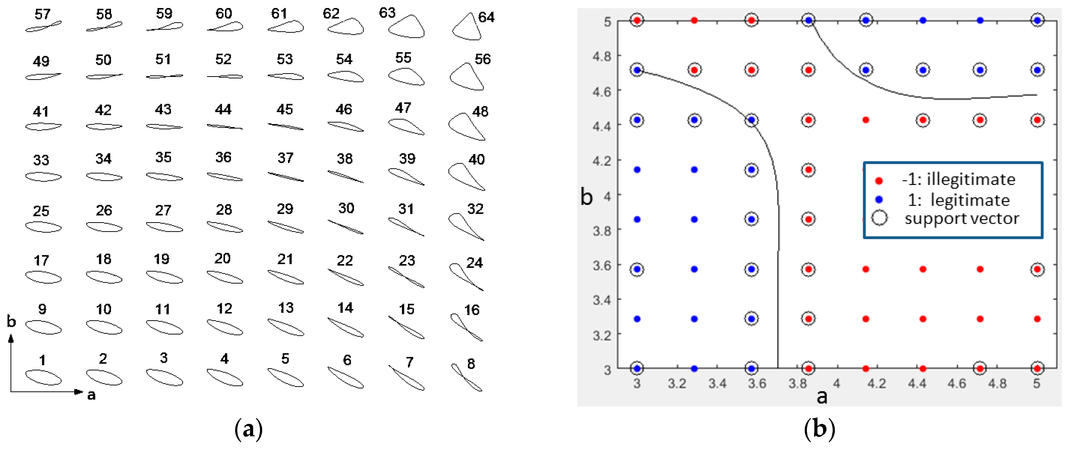
It all starts with a small portion of examples. We arbitrarily choose the dimensional parameters a and b to form a mesh of grids. Each of them possesses eight points uniformly distributed over [
3,
5], i.e., [3, 3.2857, 3.5714, 3.8571, 4.1429, 4.4286, 4.7143, 5]. Then a mesh of grids formed by [a, b] consists of 64 points, each of which associates with an orbit as shown in
Figure 5a where the rest of parameters are set to be c = 3, d = 3.1111, S
x = 3, S
y = 0.6667.
At this preliminary stage, we could boldly categorize the orbits based upon our intuitiveness. Consequently, the orbits in
Figure 5a labeled with 1, 2, 3, 9, 10, 11, 17, 18, 19, 25, 26, 27, 33, 34, 35, 41, 42, 43, 49, 53, 54, 55, 56, 60, 61, 62, 63, 64 are attributed to the legitimate class, while the others are defined as the illegitimate class. In
Figure 5b, the blue and red dots stand for the legitimate and illegitimate classes, respectively.
Obviously, this set of training data cannot be separated linearly. Hence, a Gaussian kernel is applied to achieve the nonlinear separation. The model of SVM is obtained by using fitcsvm, a command of Matlab, with KernelFunction, KernelScale, Sigma, and Standardize, setting to be rbf, auto, 0.8, and true, accordingly. The decision boundary results in two black curves, as shown in
Figure 5b.
To get a grasp of how the kernel trick works, we evaluate the Equation (18) with respect to
and plot the family of its contours accordingly. In
Figure 6, the surface that is generated by the score function contains all of the data where the points of the legitimate class are distributed over the uphill, while the points of the illegitimate class are distributed over the downhill. The decision boundary is exactly the contour at the level of zero, as shown in
Figure 6. Hence, the nature of the kernel trick is to embed the input space into a higher-dimensional space, referred to as feature space or kernel space, in which the data can be linearly separable by a plane lying horizontally at level zero. The scatter diagram in
Figure 5b is in fact the top view of the stereoscopic model, as shown in
Figure 6.
So far, the SVM has manifested its great strength in classification. Taking a close look of the orbits attributed to the legitimate class, it unveils that our preference in selecting the orbits possesses three characteristics, i.e., the obliqueness of the orbit being shallow, avoiding the orbit from being too slim or too thick, and no self-intersection.
In this pilot study, the training data were prepared manually because they were inspected by our vision and judged by our intuitiveness. The judgement based on the qualitative descriptions is more or less involved with subjectivity rather than objectivity. It leads that the training data might be contaminated with some amounts of unconscious bias. How to well prepare the training data is always a vital step in the supervised machine learning techniques. Hence, the following two sections are devoted to turn those discriminant criteria from qualitative descriptions into quantitative definitions, like mathematical functions or rules, based on which the machine vision can take the place of human vision to label a large scale of orbits.
5. Obliqueness and Slenderness
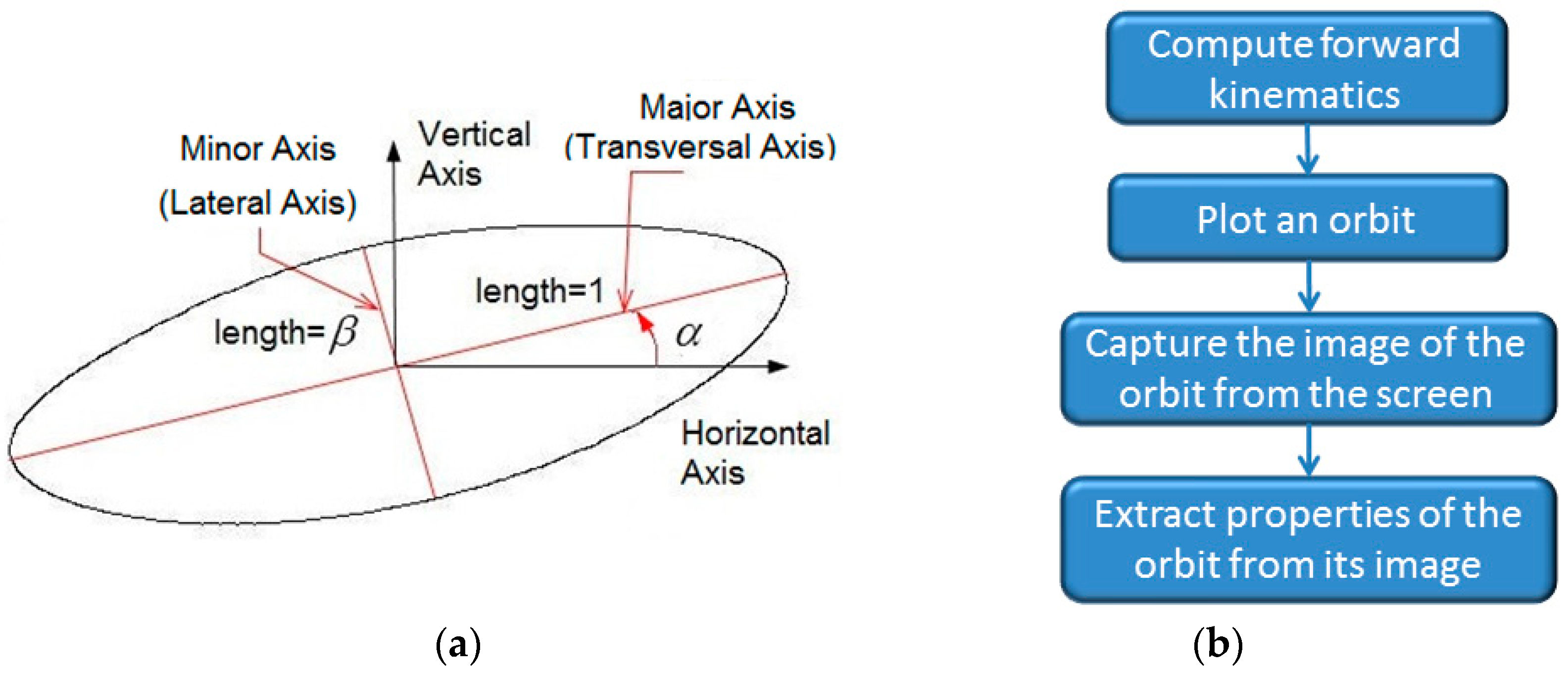
Let us define two properties of the orbit, i.e., obliqueness
and slenderness
, as shown in
Figure 7a and apply the image processing to extract these properties from it. The flowchart of extracting these properties from an orbit, as shown in
Figure 7b, includes computing the forward kinematics of the TJL using Equations (1)–(11); plotting an orbit; capturing the image of the orbit [
20,
21] from the screen; and, measuring the obliqueness
of the orbit, the length of its major axis, the length of its minor axis from its image. Subsequently, the slenderness ratio,
, of an orbit is calculated by taking the length of its minor axis divided by the length of its major axis.
After computation, the properties of the 64 orbits presented in the previous section are obtained and listed in the
Table 1. Regarding the extraction of properties, it is involved with several standard techniques of image processing [
22,
23], i.e., calculating the centroid of the image, obtaining the centroid-shifted image, computing the eigenvectors and eigenvalues of the centroid-shifted image, retaining the eigenvectors with the maximum and minimum eigenvalues, calculating the Euclidean distances and orientations or simply applying the Matlab command, regionprops.
The question remains as to whether we can deduce the criteria in terms of mathematical functions that a computer can reason about. The answer is positive, as the sequel will show. When we plot the scatter diagram according to the
Table 1, the
Figure 8a unveils that the data of the legitimate class cluster within a region that is tightly related to our preference in selecting the desired orbits. As observing the location of the clustering region, it tells that our preference is indeed consistent with the requirements of shallow obliqueness and moderated slenderness. It also confirms our skepticism of the training data contaminated with some amounts of bias because few dots of blue are aberrated from the clustering region.
In
Figure 8a, the contours are plotted according to the score function of the SVM. The contour at level 1.2 encircles a region containing a family of orbits in consistency with our preference. The mathematical criterion obtained by imposing an inequality on the score function of the SVM is called the model-based criterion. However, this set of training data are only sampled from two-dimensional parameters, i.e., a and b, is not sufficient to stand for the overall data and the orbits classified by our human vision is not objective. Hence, this model-based criterion will not be used. Instead, imposing the upper and lower bounds on
and
, i.e.,
and
, as shown in
Figure 8b to delimit the desired region, called the rule-based criteria, will be used by machine vision to reclassify the orbits in the sequel.
6. Self-Intersection
Except the obliqueness and slenderness, there is an additional factor that has to be taken into account, i.e., self-intersection. An investigation is conducted here to evaluate the feasibility of image processing to detect the self-intersection. It shows that the image processing can correctly distinguish the majority of orbits regarding self-intersection but there does exit few adverse events.
Using our human vision to inspect
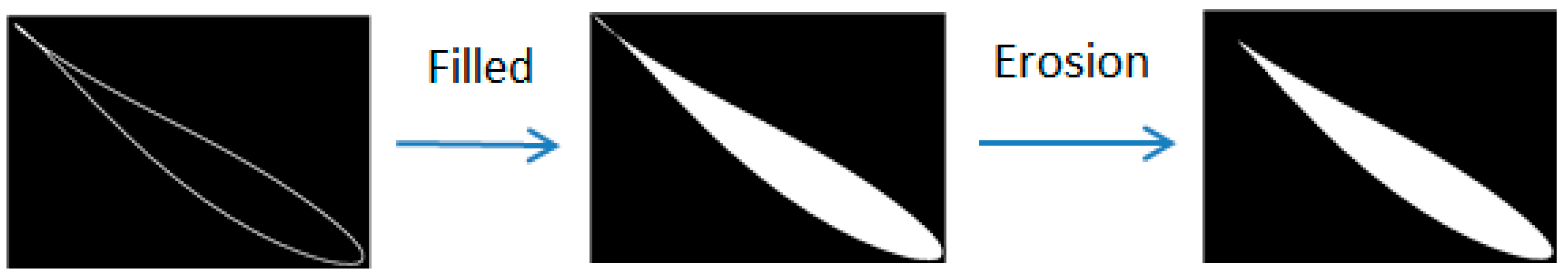
Figure 5a, the orbits with identity numbers 7, 8, 15, 16, 23, 24, 30, 31, 44, 50, 51, 52, 57, 58, and 59 are lemniscates possessing self-intersection, not acceptable for legged motion. When using the image processing to identify the self-intersection, it is achieved by the morphological erosion operation that is filling the area enclosed by the orbit, eroding the filled area with a three-by-three square structuring element, and counting the number of connected objects, as shown in
Figure 9. The orbit will be judged as no self-intersection provided that the number of objects is equal to 1. Otherwise, it is self-intersected. It turns out that the orbits with identity numbers 8, 15, 16, 22, 23, 24, 30, 31, 37, 38, 44, 45, 49, 50, 51, 52, 57, 58, 59 recognized by machine vision are self-intersected.
All of the lemniscates recognized by us have been successfully captured by machine vision, except one discrepancy on the orbit with identity number 7. The reason why it escapes from the inspection of machine vision is because it resembles a sharp-point oval before erosion and it becomes a sharp-point oval after erosion, as shown in
Figure 10.
Figure 11 shows that the non- self-intersected orbits are misjudged as self-intersection by the machine vision. Get a glimpse of
Figure 10 and
Figure 11, it seems that the image erosion encountering with the slimness undermines its identification on self-intersection.
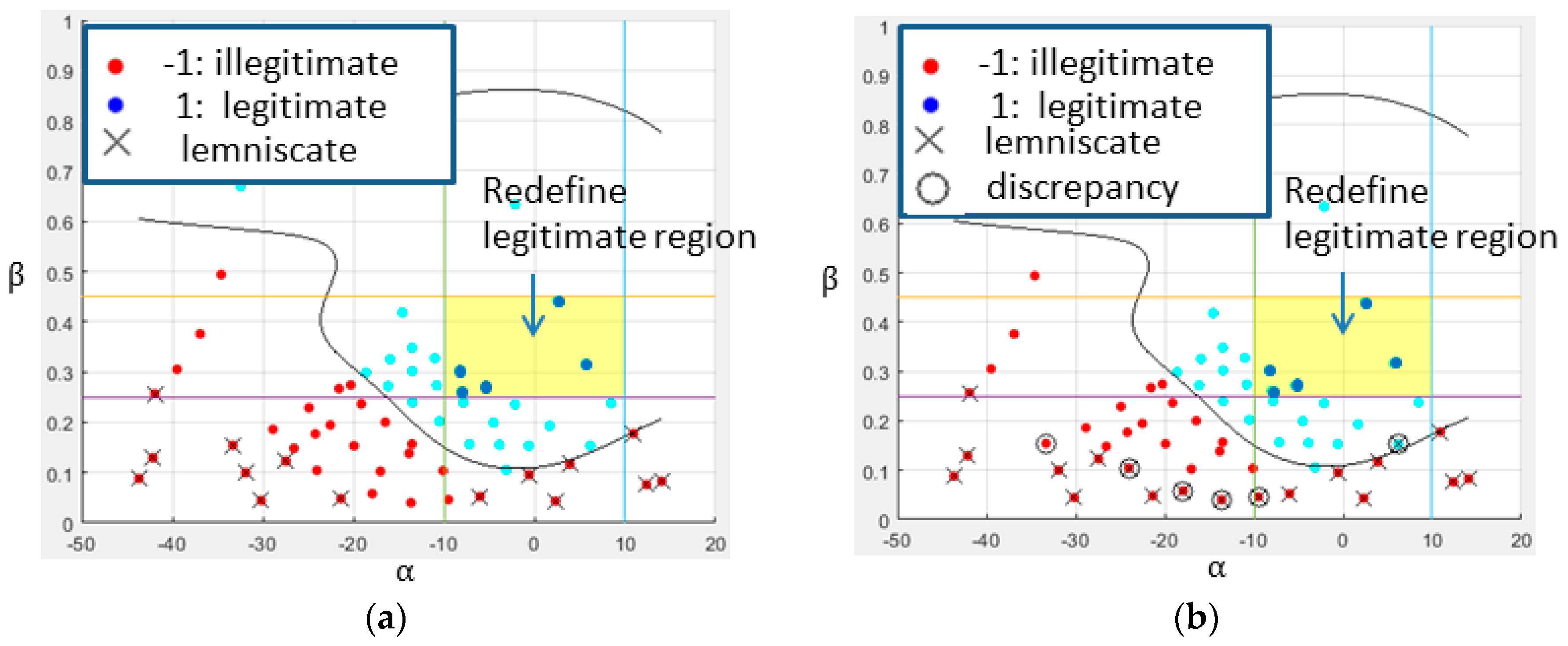
Let us examine the lemniscates that are recognized by human vision and machine vision, as shown in
Figure 12a,b, where the lemniscates are marked with the cross-X and the discrepancies are marked with the circle-O. It is clear that the lemniscates distribute over the region with a low slenderness ratio. Be reminded that, when the orbits are too slim, they will be precluded from the legitimate class and then it is meaningless to care about their self-intersection. As imposing the rule-based criteria
and
to redefine the legitimate region, all of the lemniscates are far away from that region, as shown in
Figure 12. It is sufficient to use the rule-based criteria on
and
to categorize the orbits without detecting the self-intersection.
7. Advanced Model of SVM
Obtaining a sufficient amount of training data that adequately reflects the characteristics of the field data is always the bottleneck of supervised learning. The breakthrough we made is to combine the image processing with the rule-based criteria, as shown in
Figure 13, so that the machine vision can label a vast amount of training data as well as a full-scale of data.
Note that Xp consists of properties and ; Xd consists of six dimensional parameters, i.e., , , ; and, Y is the label set. Xd and Y carry the inputs and correct outputs of the training data for SVM2, so do Xp and Y for SVM1. If each dimensional parameter is uniformly sampled into points, the number of training data associated with 6 parameters will be . Hence, we prepare four sets of training data with different numbers, i.e., 64(), 4096(), 46656(), 262144(), to train SVM1 and SVM2.
The cross-validation is the method to evaluate the performance of the trained model. In
Table 2, there is a list of losses that were obtained by 10-fold cross-validation. It shows that the SVM1 has a performance better than SVM2. As the number of training data is increased, the rate of loss is decreased.
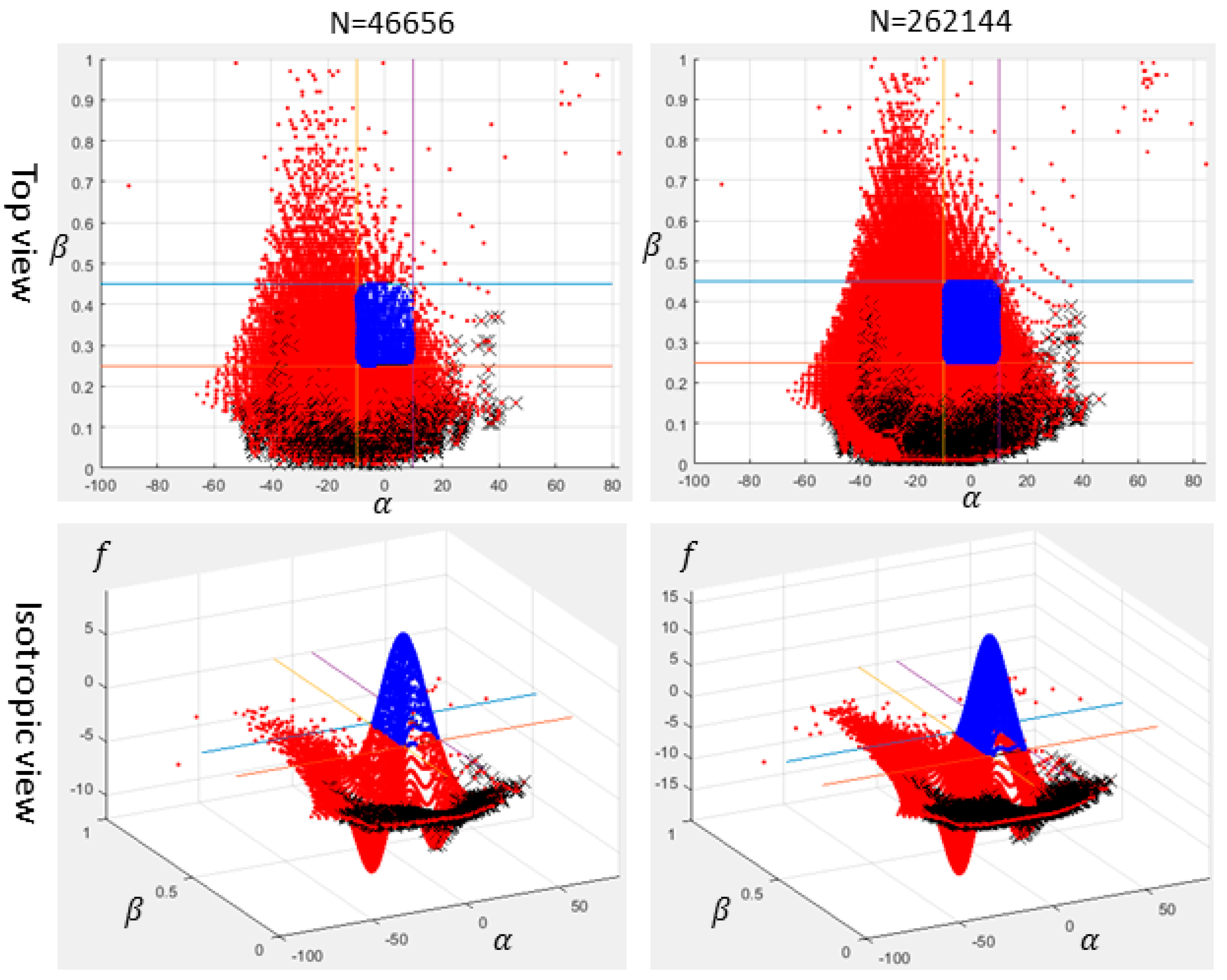
Since SVM1 is the model drawn from the training data [Xp, Y] and the input data Xp possess only two variables, its model can be visualized. However, it is not the case for SVM2 as its input data Xd possessing dimension higher than two. The scatter diagrams of SVM1 with four sets of training data are shown in
Figure 14 and
Figure 15 where the blue and red dots stand for legitimate and illegitimate classes, respectively; the black cross-X stands for the lemniscates that were identified by machine vision. Note that the diagram with 64 data is insufficient to manifest its geometrical manifold, hence some contours are added for the sake of visualization.
Recall the self-intersection addressed previously. Observing the
Figure 14 and
Figure 15, most of lemniscates marked with X indeed aggregate at the region with a slenderness ratio below 0.25. Interestingly, the lemniscates whose slenderness ratio exceeds 0.25 will also be precluded from the legitimate class by the reason of their steepness. Evidently, both slenderness and obliqueness criteria are sufficient to categorize the data.
As refining the sampling points on each dimensional parameter, either the number of training data or the computational time in property extraction prodigiously grows, as shown in
Table 3. Comparatively, each dimension sampled into six points is more pragmatic than when it is sampled into eight points, because it can provide the SVM with sufficient amount of unbias training data at the cost of less computational time.
In the framework of machine vision and SVM, as shown in
Figure 13, two databases gathering all eligible data concerned with properties of orbits and dimensions of TJLs are established. With the aid of these two databases, a program can be developed to fulfill the inverse problem. It searches the orbits in compliance with the specification of
and
from the database of properties and uses their correspondent identity numbers to list all candidates of TJLs from the database of dimensions. Undoubtedly, the database of properties has collected all the orbits with legitimate properties, i.e.,
and
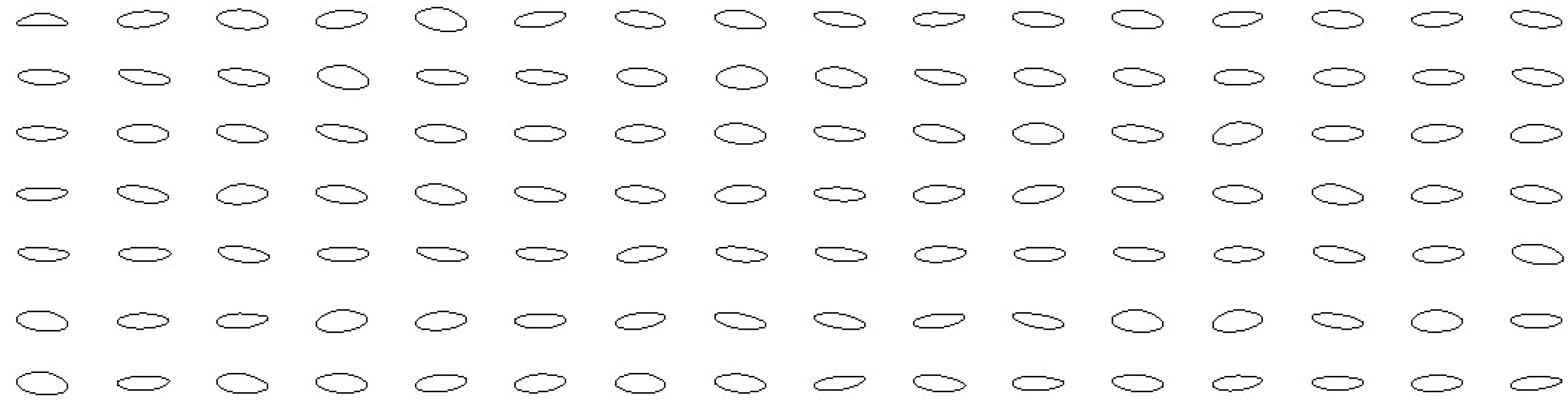
. However, what would these legitimate orbits look like? Let us randomly select the data from the database of dimensions and plot their orbits accordingly. In
Figure 16, it shows that all the orbits possessing swallow obliqueness, neither too slim nor too thick, and no self-intersection are absolutely qualified to be the foot trajectories for the legged robots. Hence, the designer can refer to the database to determine the dimensions of TJLs without a risk of rendering an illegible design.
In
Table 3, the number of training data is 262144, as each dimension is sampled into eight points. The orbits in
Figure 2 are randomly selected from that 262144 training data while the orbits in
Figure 16 are randomly selected from the legitimate class, which is only 10.63% of the training data. As comparing
Figure 16 with
Figure 2, it evidently shows that the machine vision has effectively classified a vast amount of orbits and successfully gathered all legitimate ones in the database.
8. Conclusions
Theo Jansen linkage is an appealing mechanism to implement a bio-inspired motion for a legged robot. The oval orbit generated by the Theo Jansen linkage, possessing a transversal axis longer than a lateral axis, achieves energy efficient walking as comparing to the circular orbit generated by the four-bar linkage. However, the patterns of orbits that are produced by the TJL may vary according to its ensemble dimension and can be casted into four groups, such as bell curves, ovals, sharp-pointed ovals, and lemniscates. Some orbits can be used as the foot trajectories for legged robots but some cannot. Overall speaking, the ovals or bell orbits are legitimate and the sharp-pointed ovals are partly legitimate, nevertheless the lemniscates are illegitimate.
All of academic works relevant to TJLs mainly focus on the analysis of forward problems, like kinematics, dynamics, and controls. None have ever addressed the issue of design that has to rely on the knowledge of inverse problems. To design a Theo Jansen linkage, which can generate a foot trajectory to achieve an energy efficient walking, relies on successfully sizing its eight links. It is equivalent to determine its six dimensional parameters according to the specification of orbits. Due to the complexity of TJLs, it is impossible to derive any inverse function analytically. As resorting to the numerical scheme, the heterogeneous patterns of orbits hinder the Levenberg–Marquardt method from prevailing because it is lacking capability to tell the patterns of orbits.
In order to discriminate the orbits, the machine learning technique, called SVM, is employed. The SVM gives a geometric perspective that is finding the equation for a hyperplane to best separate the different classes in the feature space, solves the convex optimization problem analytically, and hence always returns the same optimal hyperplane. Obtaining a sufficient amount of training data that adequately reflects the characteristics of the field data is always the bottleneck of supervised learning. The breakthrough that we made is to apply the image processing to label a vast amount of training data without bias.
The proposed method is divided into two steps. First, a preliminary model is built with a small portion of data to conduct a pilot study on discovering the knowledge of data. Second, an advanced model is built to deal with the large scale data. Consequently, two models of SVM are trained and the two databases concerned with properties and dimensions of all eligible designs can be established. The models of SVM are used to quickly identify the eligibility of a design data and the databases provide abundant of feasible data to which a designer can refer as designing the TJLs. The inverse problem concerned with design is fulfilled by searching the orbits in compliance with the specification of obliqueness and slenderness from the database of properties and using their correspondent identity numbers to list all the candidates of TJLs from the database of dimensions. With the aid of this proposed method, the TJLs have been successfully designed and implemented on a legged robot.
There are two topics of interest for future research. First, SVM is one of discriminant technique among learning machines. In contrast to ANN (Artificial Neural Network), hyperplanes are highly dependent on the initialization and termination criteria. SVM distinguishes itself from ANN, in that it always returns the same optimal hyperplane with a large margin. Due to its successful application, we shall advance to other ML techniques, like K-Means clustering, K-Nearest Neighbors, Naive Bayes, and Random Forest, etc., and evaluate their merits and demerits. Second, the structure of a TJL can be improved by replacing two isosceles right triangles with two right triangles. The image processing shall extract more properties from the orbits so as to discriminate the bell curves, ovals, sharp-pointed ovals, and lemniscates. The significance of this research is to tackle the mechanism problem by means of the machine learning and machine vision.


