1. Introduction
Since the establishment of the first induced pluripotent stem cell line, many research groups have attempted to use the self-renewal ability and pluripotency of differentiated neural stem cells (NSCs) for the treatment of neurodegenerative diseases, including Alzheimer’s disease, amyotrophic lateral sclerosis, and Parkinson’s disease [
1,
2,
3,
4], and to prevent secondary degeneration in spinal cord injury [
5,
6]. The most common approach is to transplant NSCs into affected tissues [
7,
8]; therefore, it is necessary to accurately confirm their differentiation status at the single-cell level both before and after transplantation [
9]. Conventionally, NSC differentiation status is determined by examining the shape of the cells by using bright-field microscopy or fluorescent markers of neural differentiation [
10,
11]; however, these approaches are not ideal: using cell shape as an indication of differentiation status has low reproducibility due to differences in technician experience, and the fluorophores used in fluorescent markers can have lethal effects in patients [
12]. Thus, a method for discriminating differentiated from undifferentiated NSCs that has high reproducibility and is non-invasive is needed.
Various machine learning-based approaches that use photomicrographs or other images to accomplish biological and medical tasks, including the differentiation status of NSCs, have been proposed [
13,
14]. These methods are automatic, have high reproducibility, and are non-invasive to cells because fluorescent markers are not needed [
15]. Convolutional neural networks (CNNs), which are deep learning-based networks, are capable can achieve extraordinary outcomes when applied to image analysis and identification tasks [
16,
17]. For example, for the identification of differentiated and undifferentiated endothelial cells, Kusumoto et al. have developed a CNN-based algorithm that has an accuracy of 91.3% and an F-measure (weighted harmonic mean of the precision and the recall of the classification) of 80.9%. However, they did not optimize the hyper-parameters of their neural network, and the algorithm was applied at the cell-population level, not the single-cell level.
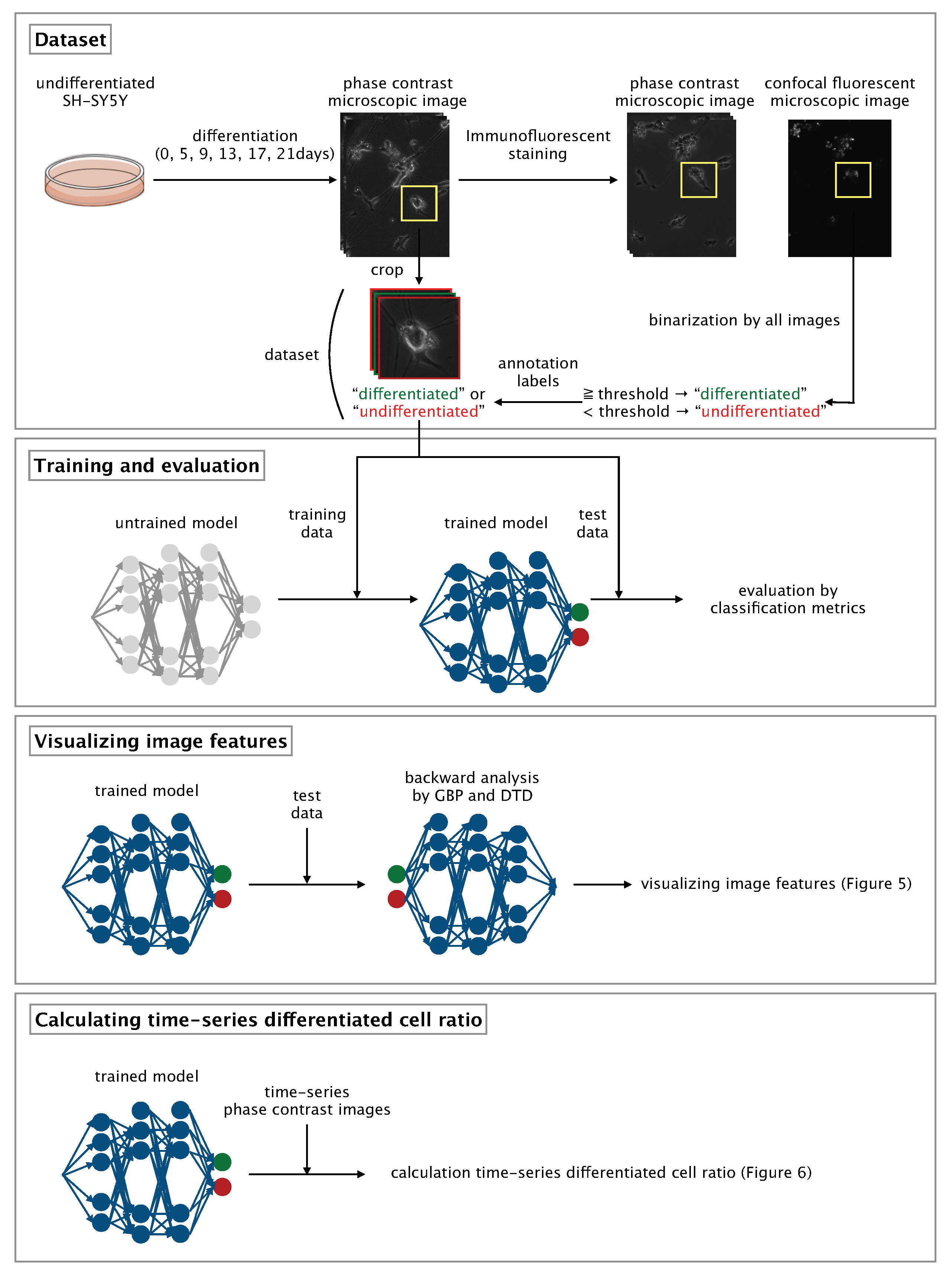
Here, we developed a CNN-based algorithm that uses phase-contrast photomicrographs of single NSCs to non-invasively determine differentiation status at the single-cell level (
Figure 1).
2. Materials and Methods
2.1. Cell Culture and Induction of Neural Differentiation in SH-SY5Y Cells
SH-SY5Y cells, which are a subline thrice-cloned from the human bone marrow biopsy-derived cell line SK-N-SH from the European Collection of Cell Cultures Cell Bank (Cat. No. is 94030304), were obtained. SH-SY5Y cells were cultured in a 1:1 mixture of Dulbecco’s modified Eagle’s medium/Ham’s F-12 Nutrient Mixture (DMEMF-12; Life Technologies, Tokyo, Japan) supplemented with 15% (vol/vol) heat-inactivated fetal bovine serum in a 5% CO
incubator at 37
C. For all experiments, cells were subcultured in a 35-mm glass-based dish (Iwaki, Tokyo, Japan) coated with collagen (Cellmatrix Type IV; Nitta Gelatin, Osaka, Japan). To induce neural differentiation, all-trans retinoic acid (Sigma-Aldrich, St. Louis, MO, USA) was added to the SH-SY5Y cells at a final concentration of 10
M in DMEMF-12 with 15% fetal bovine serum (day 0 after induction of differentiation) every two days for 5 days (0, 2, 4 days), after which the cells were incubated with 50 ng/mL brain-derived neurotrophic factor (Sigma-Aldrich) in DMEMF-12 (without serum) [
18]. The cells were incubated in DMEMF-12 for a total of 0, 5, 9, 13, 17, or 21 days.
2.2. Phase-Contrast Photomicrographs of SH-SY5Y Cells before Immunofluorescent Staining
After the induction of differentiation and incubation, phase-contrast photomicrographs of the SH-SY5Y cells were obtained by using a phase-contrast microscope (IX81; Olympus, Tokyo, Japan) equipped with a 20× objective lens and an on-stage incubation chamber (INUG2-ONICS; Tokai Hit, Shizuoka, Japan); the temperature and CO concentration were maintained at 37 C and 5%, respectively. The phase-contrast photomicrographs were recorded with a CMOS camera (ORCA-Flash4.0; Hamamatsu, Shizuoka, Japan).
2.3. Immunofluorescent Staining
After the phase-contrast photomicrographs of the SH-SY5Y cells were obtained, the cells were fixed with 4% paraformaldehyde (Wako, Osaka, Japan) for 15 min at room temperature and then permeabilized by incubating in phosphate-buffered saline (PBS; Wako) containing 0.1% Triton X-100 (Alfa Aesar, Haverhill, MA, USA) for 10 min at room temperature. The cells were then blocked by incubating in PBS containing 1% bovine serum albumin (Wako) for 30 min at room temperature. To distinguish between differentiated and undifferentiated cells, synaptophysin, a marker of mature neuronal cells, was used. Synaptophysin is a synaptic protein that plays a role in the synaptic transmission of neurotransmitters in the mature synapse [
19]; therefore, it can be used as a marker of mature neuronal cells. The expression of synaptophysin has also been confirmed in differentiated SH-SY5Y cells [
20]. Primary antibody (mouse monoclonal anti-synaptophysin [1:500; Abcam, Cambridge, UK]) was diluted with 1% bovine serum albumin in PBS and added to the cells, and the cells were incubated for 120 min at room temperature. After incubation, a secondary antibody (donkey anti-mouse-IgG [H+L] conjugated with Alexa Fluor 488 [a21202, 1:1000; Life Technologies]) was diluted 1:1000 with 1% bovine serum albumin in PBS, added to the cells, and the cells were incubated for 60 min at room temperature.
2.4. Photomicrographs of SH-SY5Y Cells after Immunofluorescent Staining
After immunofluorescent staining, images of the SH-SY5Y cells were recorded under a phase-contrast microscope equipped with a confocal scanner laser unit (CSU22; Yokogawa, Tokyo, Japan) and a 10× objective lens. Then, the photomicrographs of each SH-SY5Y cell before and after immunofluorescent staining were matched by visual observation.
2.5. Photomicrograph Labeling and Dataset Compilation
Each photomicrograph of a single, immunostained SH-SY5Y cell was labeled as ‘differentiated’ or ‘undifferentiated’ according to the synaptophysin intensity of the cell. In each photomicrograph, the area containing the cell was selected manually and saved by using the ROI (region of interest) Manager function within the Fiji image processing package [
21]. The threshold of synaptophysin intensity for distinguishing between differentiated and undifferentiated cells was determined by means of Otsu thresholding [
22]; images of cells with a synaptophysin intensity equal to or greater than the threshold were labeled as ‘differentiated’ and those of cells with a synaptophysin intensity less than the threshold were labeled as ‘undifferentiated’. After labeling, the phase-contrast photomicrographs obtained before immunostaining were manually cropped to 400 × 400 pixels with a single cell at the center of the image and then resized to 200 × 200 pixels to afford a dataset comprising 176 annotated, cropped, phase-contrast photomicrographs of individual, non-immunostained, differentiated or undifferentiated SH-SY5Y cells.
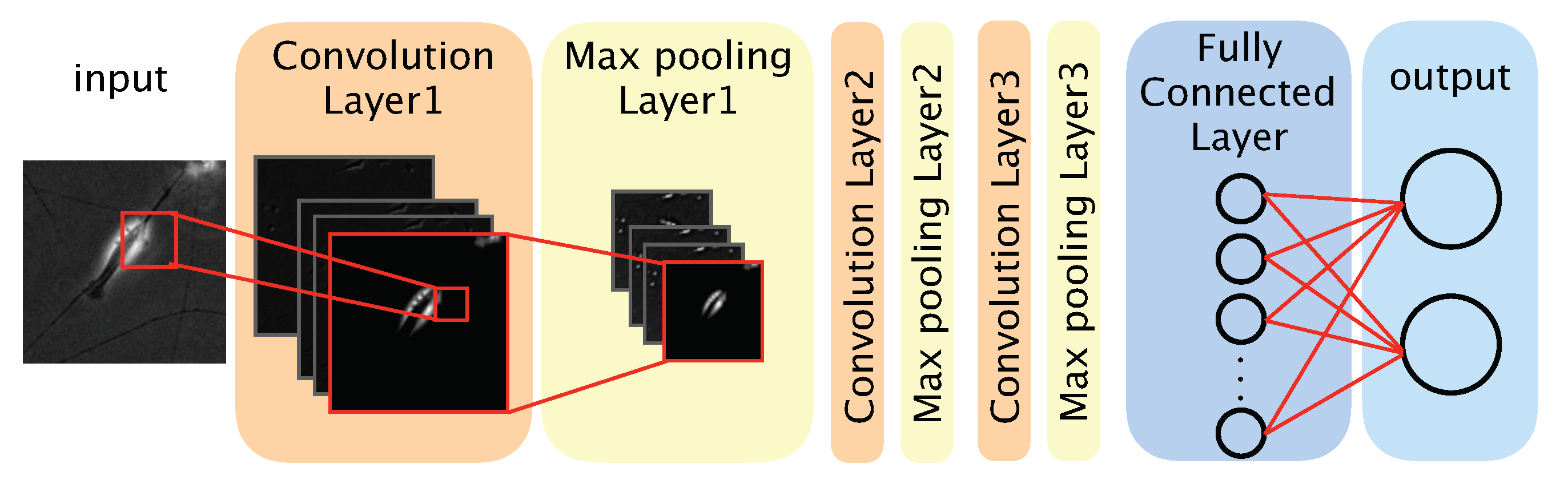
2.6. Architecture of the CNN-Based Model
We used a CNN-based model to distinguish between differentiated and undifferentiated cells in the photomicrograph dataset (
Figure 2). The model comprised three convolution layers, three max pooling layers, a fully connected layer, and an output layer. The convolution layers each applied a convolution filter to the input image and feature maps to extract features. We defined a feature map as a downscaled image that was obtained by a layer. Convolution filters were optimized during the training phase, and the optimized filters were used during the test phase. The max pooling layer was used to improve the position invariance by downscaling the feature map. We used the ReLU (rectified linear unit) function, a nonlinear function, as the activation function for each convolution layer and the fully connected layer. The output layer comprised two neurons, each corresponding to one classification (‘differentiated’ or ‘undifferentiated’). To obtain the probability of a given image showing a differentiated or undifferentiated cell, we used the softmax function as the activation function of the output layer. The class (‘differentiated’ or ‘undifferentiated’) with the highest probability was considered the output of the model. The source code of our algorithm is available at:
https://github.com/funalab/CoND.
2.7. Training and Evaluation
Our model was trained and evaluated by using four-fold cross-validation and our compiled dataset (training:test = 3:1). The intensity values of the phase-contrast photomicrographs were normalized to the median [
23]. In the training phase, the batch size was set to two, and the training data (phase-contrast photomicrographs and labels) were input as two batches. The objective function of our model, cross-entropy loss function, was defined as
where
denotes the label as a one-hot vector corresponding to the
nth image in the batch,
denotes the output of the
nth image, and
N denotes the batch size. We used the Adam optimization algorithm in order to avoid local minimum solutions [
24]. We used HeNormal [
25] to initialize the weights. To prevent over-learning, which is a problem when the number of training samples is small, the data were increased by rotating each training image 90
, 180
, and 270
. We also added Dropout to the first fully connected layer to prevent overfitting [
26]. For training, the number of epochs was fixed at 100.
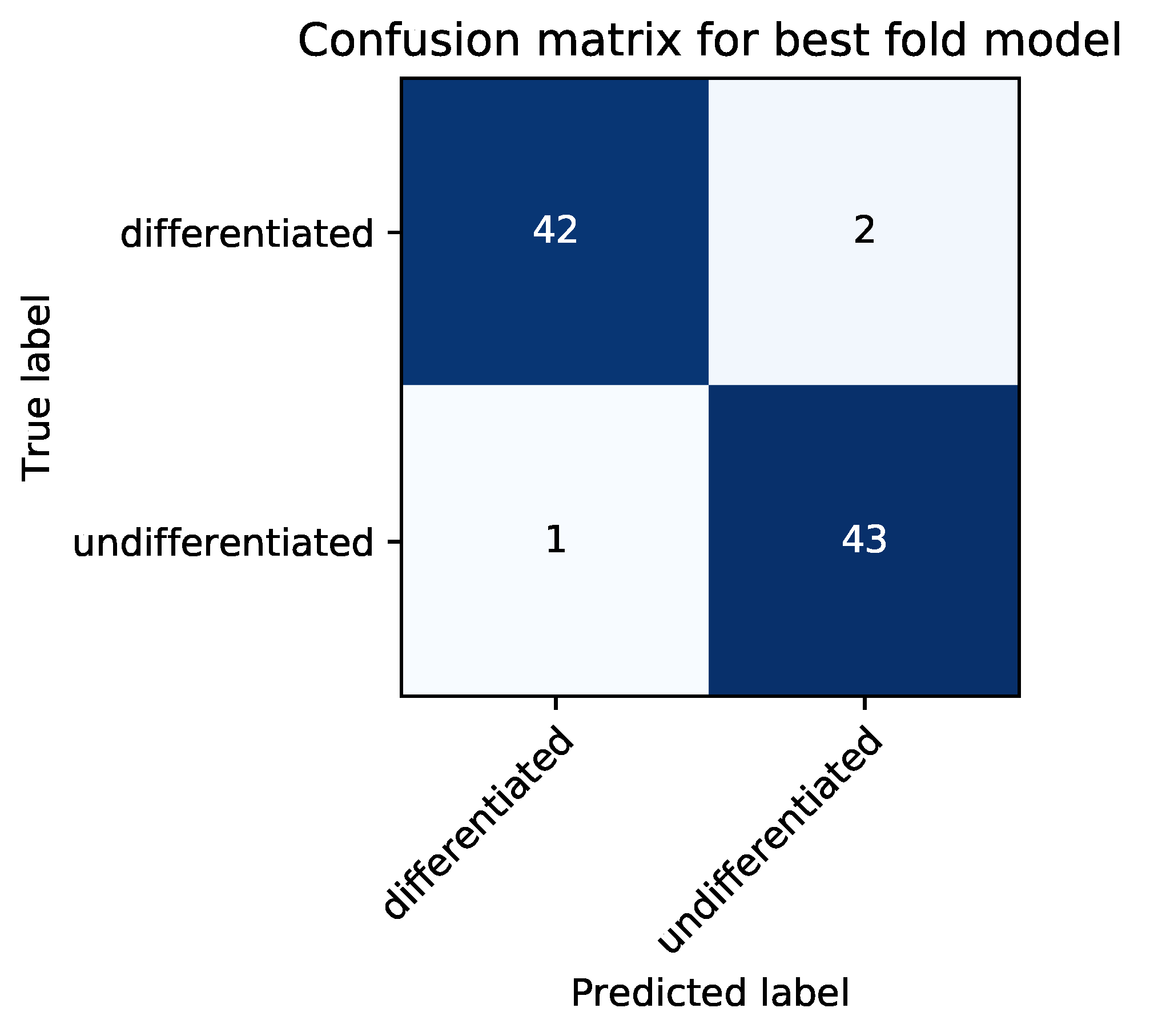
2.8. Classification Metrics
In the test phase, the classification accuracy of our model was evaluated by using test data. An answer was considered correct when an image of a differentiated cell was classified as such (true positive, TP) or an image of an undifferentiated cell was classified as such (true negative, TN). An answer was considered incorrect when an image of an undifferentiated cell was classified as a differentiated cell (false positive, FP) or an image of a differentiated cell was classified as an undifferentiated cell (false negative, FN). As evaluation metrics, we used average classification accuracy (ACA), recall, precision, specificity, and F-measure, which were defined as follows:
We set the highest ACA score during epoch for each cross-validation. At this epoch, we calculated recall, precision, specificity, and F-measure for each cross-validation. We implemented our CNN model in Python 3.6 and used Chainer [
27], which is an open-source deep-learning framework. We used an NVIDIA Tesla P100 (1189 MHz, 9.3 TFLOPS) graphics processing unit for the learning and classification calculations; the P100 was connected to Reedbush-H, the calculation server of the University of Tokyo Information Infrastructure Center, Tokyo, Japan.
2.9. Hyperparameter Optimization
We used the SigOpt optimization platform to optimize the hyperparameters of our CNN model [
28]. The best value during 30 epochs was used for each parameter (
Table 1).
2.10. Visualization of the Informative Features Learned by Our Model
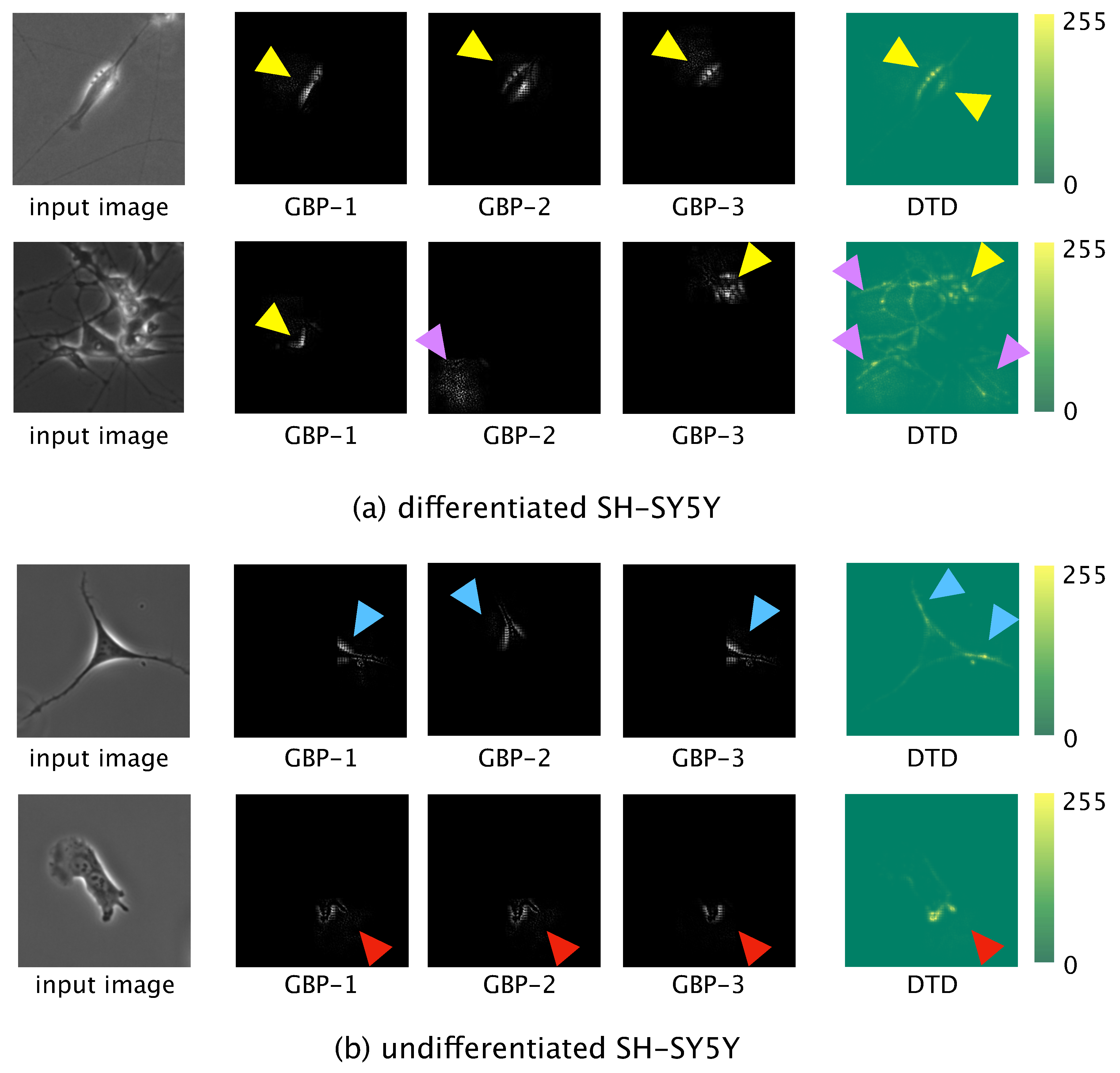
Locally informative features were visualized by using guided backpropagation (GBP) [
29], and globally informative features were visualized by using deep Taylor decomposition (DTD) [
30]. For the GBP, the test data were input to the trained model and forward propagation was conducted. The output value of the final convolution layer in the forward propagation was then backpropagated to an input space. The learned network then produced output of locally informative features learned. We used the three most significant values, which values were backpropagated to the input space to obtain the three most informative features.
For the DTD, a phase-contrast photomicrograph containing a single SH-SY5Y cell was input to the trained model and the output, , calculated by the softmax function after forward propagation, was obtained. was decomposed based on the weight and feature map in each layer in the direction of the input. The relevance to of each pixel of the input photomicrograph was calculated. Finally, we visualized the pixel-wise relevance of the whole image as a heatmap and acquired the globally informative features learned.
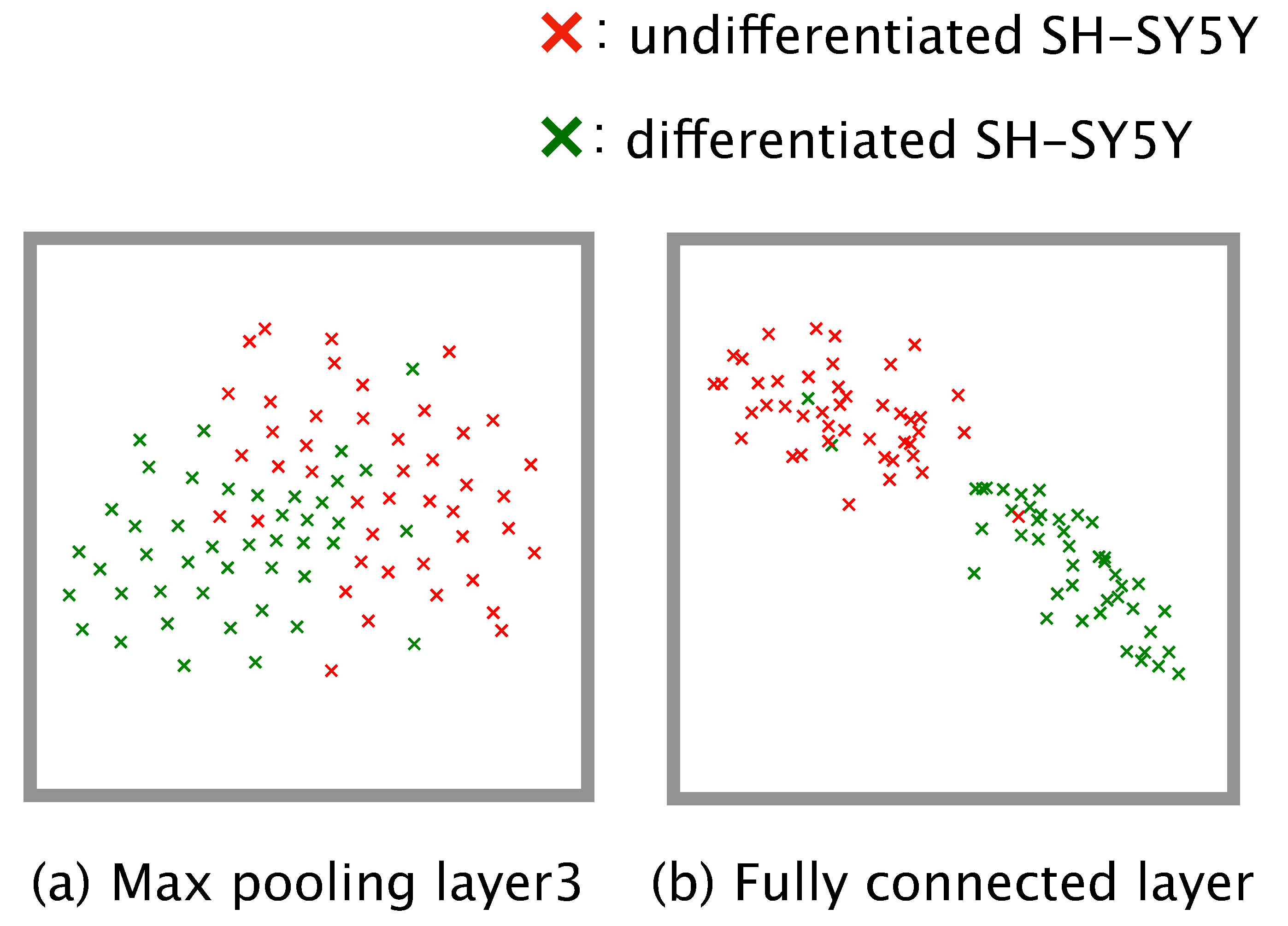
2.11. Visualization of the Training Progress
Dimension reduction is a practical means of understanding how a complex model such as a neural network executes a given classification task. We conducted dimension reduction for the feature map obtained from our trained model. The number of dimensions of the feature map was reduced to two by means of t-distributed stochastic neighbor embedding (t-SNE) [
31]. To check the global distribution of the data labeled ‘differentiated’ or ‘undifferentiated’, we input the test data from the four-fold cross-validation to the trained model, and the dimensions of the feature map output from the third max pooling layer and the fully connected layer were reduced.
2.12. Observation of Differentiation Ratio over Time
Images of SH-SY5Y cells cultured for a total of 22 days after induction of differentiation were observed every second day by phase-contrast microscopy using a 10× objective lens. Each image was manually cropped to 200 × 200 pixels with a single SH-SY5Y cell at the center. The images were then input to the trained model and classified as ‘differentiated’ or ‘undifferentiated’. The differentiation ratio, which we defined as the ratio of the number of images classified as ‘differentiated’ to total number of images classified as ‘differentiated’ and ‘undifferentiated’, was then calculated for each day the images were recorded. To confirm that there was gradual differentiation once differentiation was induced, we obtained the feature map output from the fully connected layer of our trained model using all of the phase-contrast photomicrographs (i.e., test data + time-series data). The number of dimensions of the obtained feature map were reduced to two by t-SNE. The distribution of the obtained feature map was visualized in the two-dimensional space as a scatter plot.
4. Discussion
Image resolution is considered as one factor which influences classification accuracy in bio-image analysis. To confirm the optimal image resolution to distinguish single differentiated or undifferentiated cell, we compared results obtained from (i) the original image resolution of 400 × 400 pixels, and reduced image resolutions of (ii) 200 × 200 pixels and (iii) 100 × 100 pixels by performing model learning and confirming classification accuracy. The ACA obtained from the original (400 × 400) and reduced resolution images (200 × 200, 100 × 100) were 94.9 ± 1.9%, 94.3 ± 2.1% and 86.4 ± 2.1%, respectively. Whereas the ACA obtained for 400 × 400 and 200 × 200 pixel images were within the standard deviation, the ACA obtained for the 100 × 100 image was considerably smaller than that obtained for the 200 × 200 pixel image. This indicates the model learning performs similarly for 400 × 400 and 200 × 200 pixel resolution images and does not affect the ACA classification of differentiated and undifferentiated cells. In terms of model complexity however, the MACC obtained for 400 × 400 pixel images was 14,247,901,062, which was 2.5 times higher than the MACC obtained for 200 × 200 pixel image. These results support the validity of using 200 × 200 down-scaled resolution used in our study to distinguish differentiated and undifferentiated cells.
Our CNN model achieved an ACA of 94.3% and an F-measure of 94.3%; these values are higher than those reported previously by Kusumoto et al. for a similar model [
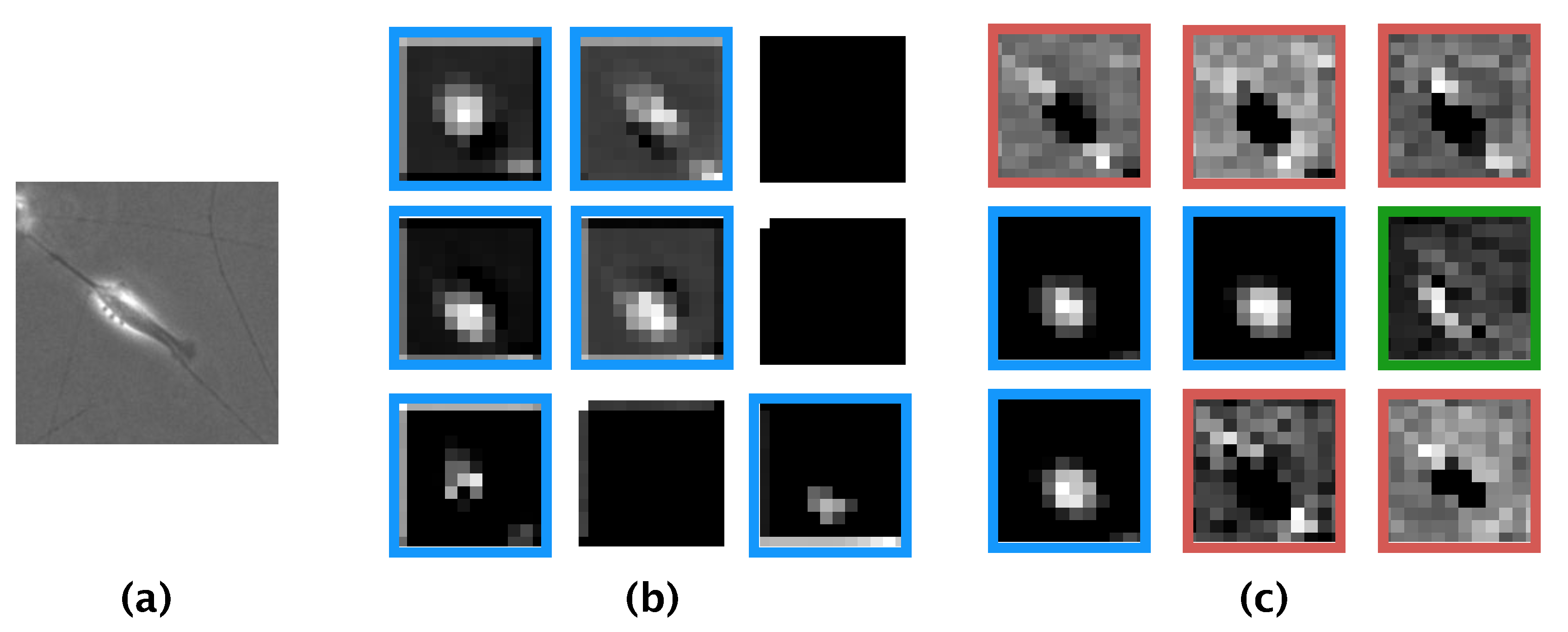
16]. Comparing the features learned by our model and those learned by the model of Kusumoto et al., we visualized the feature map output from the pooling layer of both models using the same image of a differentiated SH-SY5Y cell (
Figure 8a). The feature map produced by the model of Kusumoto et al. showed that only the halo region was considered an informative feature for the differentiated cell (
Figure 8b). In contrast, the feature map produced by our model showed three informative features: halo regions, elongated neurites, and the shape of the edge of the cell (
Figure 8c). The reason our model afforded more informative features than did the model of Kusumoto et al. could be because the hyperparameters of our model, such as the size of the filter used in the convolution layer and the stride width, were optimized and thus prevented our model from missing informative features. The higher accuracy and F-measure produced by our model compared with that of Kusumoto et al. could then be explained by the greater number of informative features learned. Of the extracted informative features for differentiated SH-SY5Y cells, a strong halo of bright light is generally observed in phase-contrast photomicrographs after the induction of differentiation [
18], and neurites are well-known to elongate during differentiation. Thus, based on our present knowledge, the informative features learned by our model were biologically relevant to differentiated SH-SY5Y cells.
As informative features for undifferentiated cells, short dendrites and the shape of the edge of the cell were learned by our model. A previous study reported that the dendrites of SH-SY5Y cells after exposure to 10
M of all-trans retinoic acid remained immature with a length of 10–40
m [
29]. In addition, it has been confirmed that during neurite elongation actin and microtubules become exposed at the surface of the cell due to destruction of the reticulated actin cortex [
32]. This indicates that dendrite elongation begins at the edge of the cell, and would explain why the shape of the edge of the cell was learned as an informative feature of undifferentiated cells. To verify this hypothesis, additional studies using actin staining are needed to check that such features of the cell edge do actually become neurites.
In the present study, photomicrograph imaging of single SH-SY5Y cells comprised the learning data for differentiation classification of cells. This study has indicated that the inhomogeneous differentiation status of each cell can be distinguished by its CNN model, through recognising critical distinct morphological features. When cellular differentiation is induced in vitro, this is usually carried out in densely cultured cells. The work of Kusumoto et al. demonstrated that differentiation status could be accurately classified in inhomogeneously differentiated densely cultured cells [
16]. The present study focused primarily on the cellular morphological features and their relationship to differentiation status. Further work is needed to clarify whether the CNN model developed in the present study is able to accurately classify differentiation status in inhomogeneously differentiated densely cultured cells.
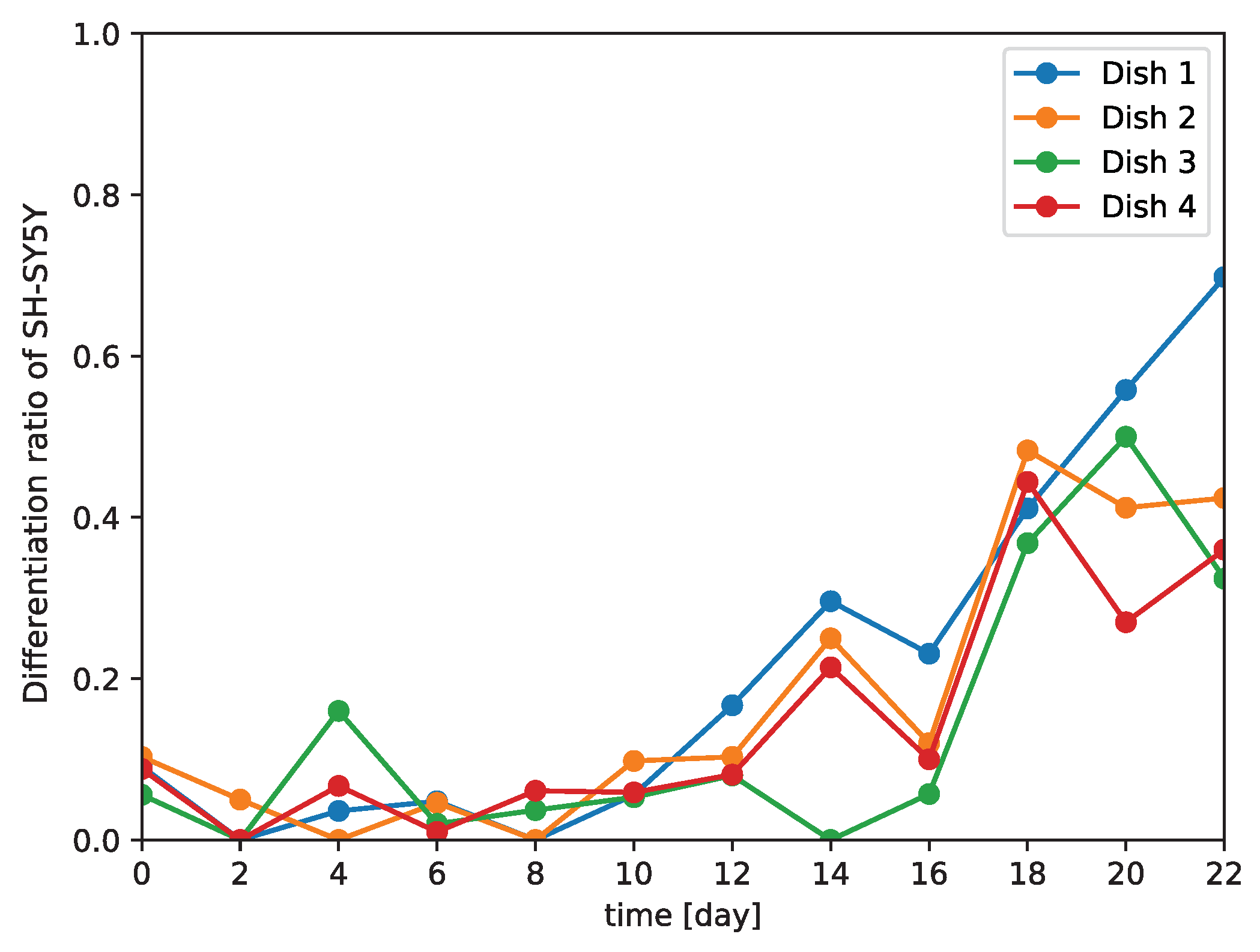
Because our model is a non-invasive means of distinguishing between differentiated and undifferentiated SH-SY5Y cells, we examined the differentiation of SH-SY5Y cells over time (
Figure 6). We observed that the number of differentiated cells began to increase at 10 days after the induction of differentiation. A previous study demonstrated that 90% of SH-SY5Y cells stopped proliferating at five or three days after the addition of all-trans retinoic acid or brain-derived neurotrophic factor, respectively, with most of the cells arrested in the G1 phase; it was speculated that these arrested cells gradually began to differentiate from that time point on [
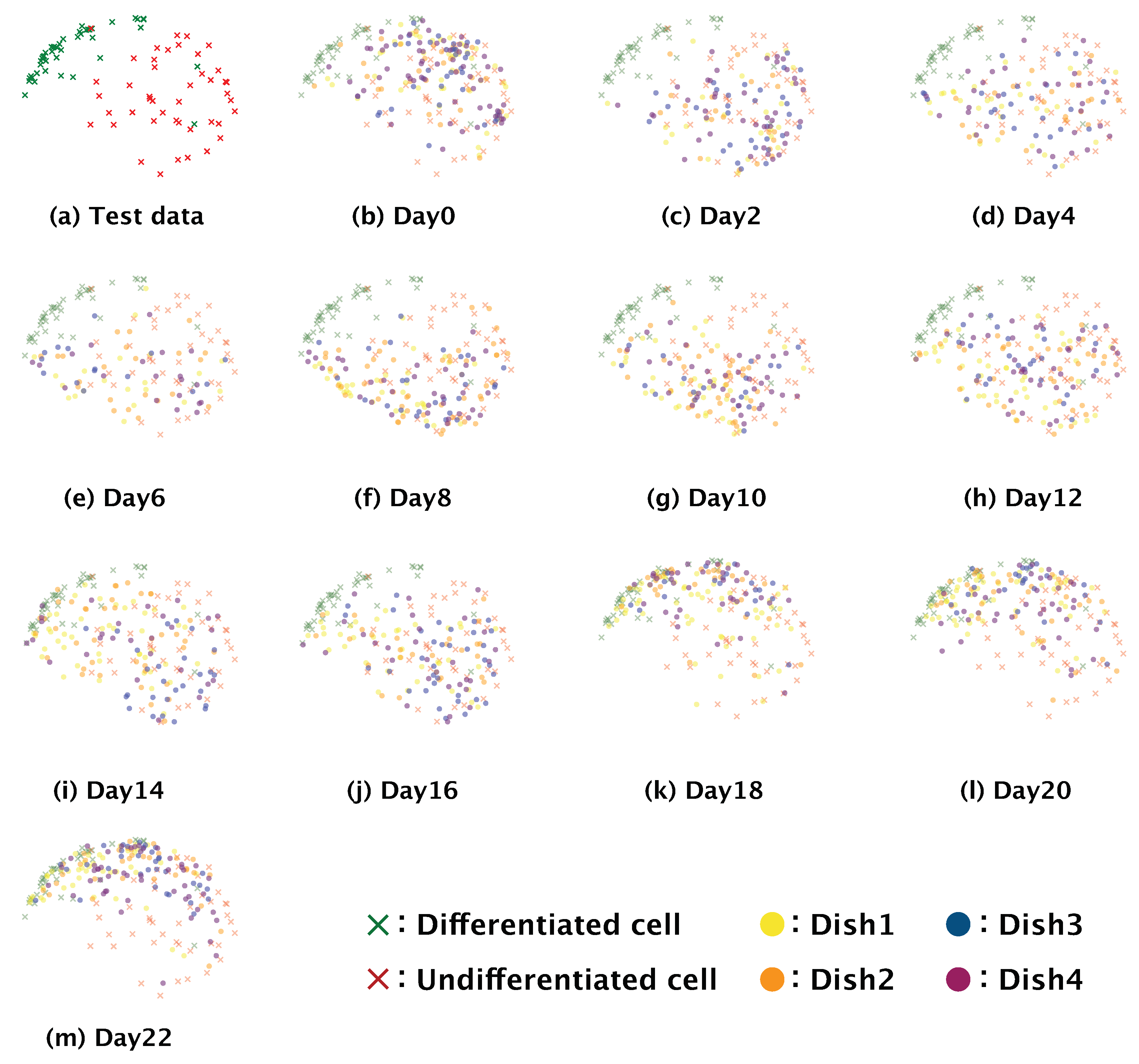
18]. We hypothesize that the increase in differentiation we observed at 10 days after the induction of differentiation could be related to this phenomenon. The gradual differentiation of SH-SY5Y cells after day 10 was also confirmed by the distributions of the feature maps output from the fully connected layer in the two-dimensional space using t-SNE; the distributions of the feature maps for days two to eight (
Figure 7b–f) showed a greater ratio of undifferentiated cells, whereas those for day 10 onwards showed a greater ratio of differentiated cells (
Figure 7g–m). These results support that our model could correctly identify the start of and gradual progression of differentiation in SH-SY5Y cells. Our data also showed that the differentiation ratio fluctuated over time depending on the subculture (
Figure 6). This implies that differentiation proceeds at different rates in different subcultures, and so generalizations about the rate of differentiation of SH-SY5Y cells cannot be made.
A number of effective network architectures exist for a learning dataset of photomicrographs in a time-series in order to acquire a differentiation ratio over time (
Figure 6). These include long short term memory (LSTM) and recurrent neural network (RNN). Previous research has demonstrated that a learning model consisting of CNN and LSTM can detect cells in mitosis from phase-contrast photomicrographs in time-series [
33]. Another study created a learning model using CNN and RNN that was highly accurate in distinguishing differentiated hematopoietic stem cells from progenitor cells using time-series bright-field photomicrographs [
34]. These learning models were known to be effective for the analysis of time-series data, however they were found to be too complex to determine the most significant morphological features that informed differentiation classification. The key purpose of the current study was to identify the critical cellular morphological features that would facilitate highly accurate classification of differentiated versus undifferentiated cells. Therefore, learning models such as LSTM and RNN were not adopted in this study. A need to formalize the methodology of recognising critical cellular morphological features has been identified, and further work in this regard is required to enable differentiation classification by LSTM or RNN.
In the clinical setting, it is important to use only differentiated cells to transplant into patients. Therefore, our non-invasive image-based approach could be useful for quickly and accurately confirming the differentiation status of cells for transplantation. A limitation of the present study is that we only used a single neuronal marker (synaptophysin) to determine differentiation status by immunostaining. However, there are several other neuronal markers that we could have used, such as dopamine transporter and tyrosine hydroxylase. In the clinic, the use of multiple markers may be necessary to ensure patient safety and future studies are needed to address this issue.
Research into deep learning is progressing rapidly; therefore, a method that outperforms our algorithm in terms of accuracy will surely be proposed in the future. Even so, we believe that it is important to show how classification by feature analysis can be accomplished by using approaches such as t-SNE, GBP, and DTD for the further understanding of neural networks.

 ,
, 


