Optimized Refraction Travel Time Tomography

Abstract

In seismic refraction exploration, travel time tomography is the most widely used method in engineering and environmental geophysical exploration. In this paper, we mainly optimize the travel time tomography of refraction. First, with respect to the forward algorithm, we introduce a new travel time calculation method to improve the accuracy and efficiency of forward calculation. Based on the fast marching method (FMM), we introduce an improved forward calculation method called the multi-stencil fast marching method (MSFM). In the process of inversion, we propose a dynamic prior model composite constraint (DPMCC) method based on the T0 difference method from the idea of multi-scale inversion. Meanwhile, we use the prior information to improve the accuracy of inversion. Furthermore, we use the dynamic regularization factor selection method to make the inversion solution more stable and reliable. Finally, we test and analyze the synthetic data and the measured data to verify the effectiveness of the optimized travel time tomography algorithm.

1. Introduction

In the near-surface seismic exploration, the refraction exploration has been widely used due to its simplicity and high efficiency. The refracted wave exploration is mainly based on the basic theory that the velocity of the underlying stratum is higher than that of the overlying stratum. By recording the wave’s arrival time, the physical parameters such as the thickness and velocity of the subterranean stratum structure can be estimated. The refracted wave exploration method first appeared in the 1930s and was developed for computer automated interpretation in the 1970s [1]. At present, the engineering refracted wave method is commonly used to detect the thickness of the cover layer [2], study the undulation of the bedrock surface [3], identify the hidden fault, measure the depth of the diving surface, and detect underground cavities and tunnels [4]. Rucker pointed out that the seismic refracted wave method can provide the near-surface geological information for engineering geological applications [5]. In an actual survey, Wang applied a set of engineering seismic refracted wave exploration methods to explore dam diseases, which achieved good results [6].

Tomography was first used in the medical field. It was subsequently introduced into the field of seismic exploration. In the 1970s, Aki et al. first used the seismic first arrival tomography method to invert the deep crust structure of the Earth [7]. This method was then widely used in the study of deep structure imaging of the Earth [8,9,10,11,12,13,14,15,16]. Seismic tomography is also used in the field of engineering and exploration geophysics. Due to its dependence on ray density, cross-well tomography research has also achieved good results [17,18,19,20].

Surface tomography is mainly used to invert the near-surface velocity structure and provide an initial model for the more accurate waveform inversion method [21,22,23]. Ellefsen compared the effectiveness of phase waveform inversion and travel time tomography [24]. Li et al. introduced the first arrival wave travel tomography method based on the double square root function Equation [25]. Jordi et al. introduced wide-angle tomography methods at different scales [26]. Zelt et al. solved the model non-uniqueness problem by using the traditional minimum structure regularization technique and proved the superiority of frequency-dependent tomography (FDTT) [27].

In the forward modeling of refracting tomography, the traditional ray method is used to solve the travel time along the ray direction and then interpolate that information to obtain the travel time of each node of the underground section, but this method cannot adapt to complex underground structures [28,29,30]. Vidale proposed a method of approximating the eikonal equation by using the finite difference method [31,32]. The core idea of this method is to calculate the travel time of each node by tracing the front of the wave. After subsequent research and development, there are several kinds of travel time calculations and ray tracing methods based on high frequency approximation, such as the fast scan method (FSM) [33] and the fast marching method (FMM) [34,35].

In the process of refraction tomography inversion, regularization is usually used to overcome the instability of the inversion solution [36,37]. Fomel used the regularization method to smooth the model and obtain good results [38]. Liu et al. introduced prior information into the inversion process as well as internal constraints on the model [39]. Refraction travel time tomography utilizes the travel time information of the seismic wavefield without being affected by the characteristics of its source and detector. At the same time, the computational efficiency of refraction travel time tomography is much higher than that of the full waveform inversion method. Based on its mature theory and high efficiency, this method is widely used to establish the near-surface and deep velocity models.

Herein, in this paper, the refraction tomography method is optimized to improve the accuracy of inversion. Firstly, the T0 difference method was chosen for the prior constrained modeling for tomography. Then, a forward modeling method based on FMM is introduced which is called Multistencil fast marching method (MSFM). The accuracy and efficiency between FMM and MSFM are then compared and analyzed. Next, a composite constrained inversion method based on T0 difference method is proposed. Furthermore, we use dynamic regularization factors in inversion. We use the synthetic data for trial calculation and analysis, which results verify the effectiveness of the optimized travel time tomography algorithm. Finally, the refracted wave data of highway tunnel portal are processed, and two layers of velocity interface are found out from the results. The tunnel entrance is located at the speed interface. This problem should be considered in construction to prevent possible geological hazards at the entrance. At the same time, the practicability of the algorithm is proven, which can solve actual geological problems.

2. Methods

The technical route of this paper mainly includes the following five contents:

• First, T0 difference method is used to calculate the prior model.
• MSFM is used as forward calculation method instead of FMM.
• Inversion method.
• In the process of inversion, the combination of the smallest disturbance constraint and the smoothest constraint is used.
• Dynamic selection of regularization factor.

Therefore, the following section separately introduces the above contents.

2.1. T0 Difference Method

The T0 difference method was proposed by Hagedorn et al. [40] in 1959. It defines two time values: $t_{+}$ and $t_{-}$.

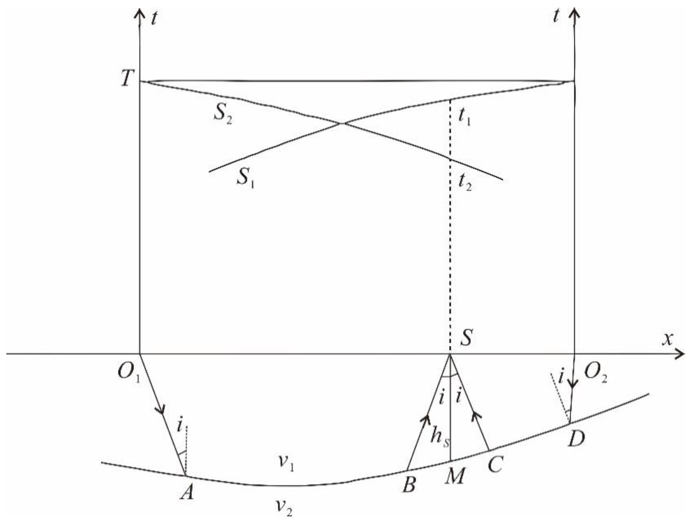
As shown in Figure 1, $i$ is the incident angle and the three ray paths are $O_{1}ABS$, $O_{2}DCS$, $O_{1}AD{O}_2$, respectively. $t_{+}$ and $t_{-}$ are expressed as:

$$t_{+}=t_{O_{1}ABS}+t_{O_{2}DCS}-t_{O_{1}AD{O}_2}$$

(1)

$$t_{-}=t_{O_{1}ABS}-t_{O_{2}DCS}+t_{O_{1}AD{O}_2}$$

(2)

We remove the same part of the ray path, $t_{+}$ can be expressed as:

$$t_{+}=t_{BS}+t_{CS}-t_{BC}$$

(3)

The interface depth of point $S$ is $h_S$, the velocity of the upper layer is $v_1$, the refractive layer velocity is $v_2$, $t_{+}$ and $h_S$ can be expressed as:

$$t_{+}=\frac{2h_s(1-{\sin }^{2}i)}{v_1\cos i}=\frac{2h_s\cos i}{v_1}$$

(4)

$$h_S=\frac{v_1}{2\cos i}{t}_{+}$$

(5)

According to Snell’s theorem, we can get the following formula:

$$h_S=\frac{v_1{v}_2}{2\sqrt{(v_2+v_1)(v_2-v_1)}}{t}_{+}$$

(6)

where $t_1$ represents the travel time of the path $O_{1}ABS$, $t_2$ represents the travel time of the path $O_{2}DCS$, $T$ represents the travel time of the path $O_{1}AD{O}_2$, then

$$t_{-}=t_1-t_2+T$$

(7)

Therefore,

$$\frac{\Delta t_{-}}{\Delta x}=\frac{\Delta t_1}{\Delta x}-\frac{\Delta t_2}{\Delta x}$$

(8)

Therefore, the apparent velocity of refraction accepted in the forward direction and the apparent velocity of refraction accepted in the reverse direction can be expressed as:

$$V_{-}^{*}=-\frac{\Delta t_2}{\Delta x}$$

(9)

$$V_{+}^{*}=\frac{\Delta t_1}{\Delta x}$$

(10)

From the apparent velocity theorem of refraction wave, Formula (8) can be obtained as follows:

$$\frac{\Delta t_{-}}{\Delta x}=\frac{2}{v_2}$$

(11)

The normal depth of refraction interface of Formula (6) can be calculated by calculating $v_2$.

Two Layer Undulating Interface Model

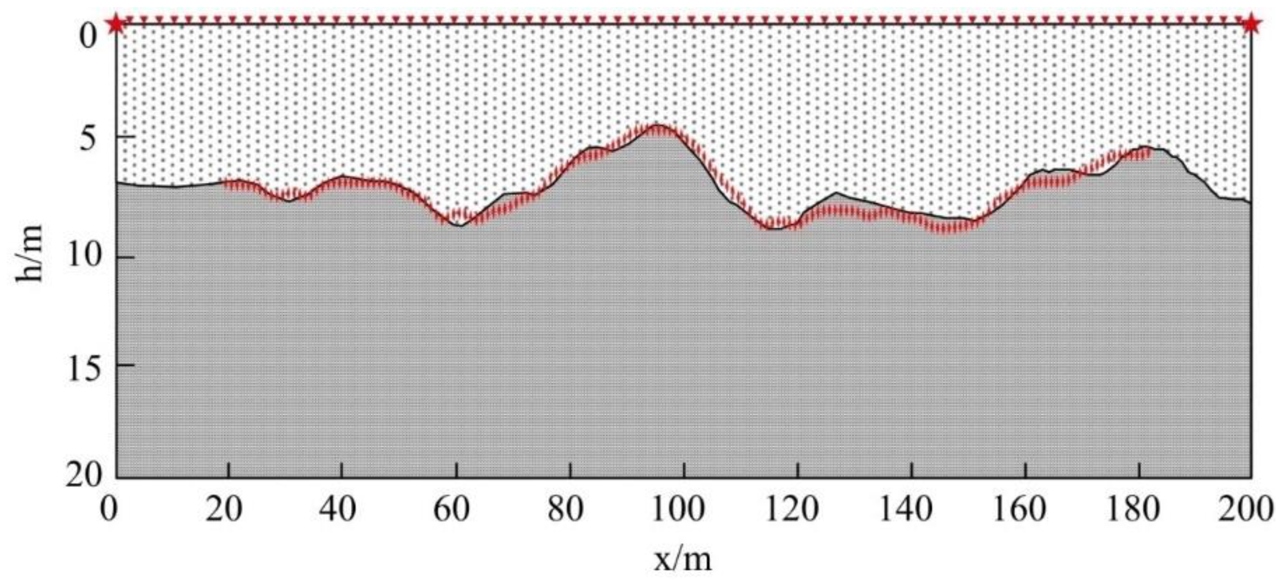
As shown in Figure 2, there are two layers of random undulating interface model. The model parameters are as follows: 200 m in the transverse direction, 20 m in the longitudinal direction, the interface depth varies from 5 m to 10 m. The velocity of the model is 1000 m/s for the first layer, the velocity of the model is 3000 m/s for the second layer. The red star shaped mark is the shot point, the red triangle mark is the detection point, the shot detection distance is 2 m, group interval is 2 m, 100 geophones.

The red prismatic points are calculated results, which are basically consistent with the random interface fluctuation of the model. The calculated velocity is 1126.9 m/s for the first layer and 2992.9 m/s for the second layer, which has a small error with the original model. Therefore, the results of T0 difference method are very accurate. Therefore, we will use T0 difference method as a prior constraint of refraction travel time tomography.

2.2. Multistencil Fast Marching Method

In order to improve the accuracy of the eikonal equation in the Cartesian domain, this paper introduces a Multistencil fast marching method (MSFM) based on FMM [41].

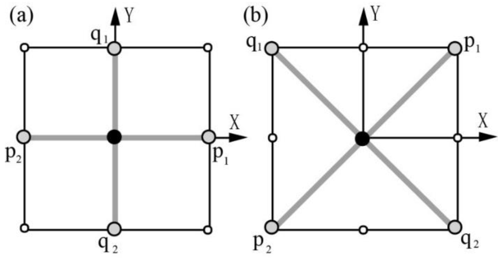
Figure 3 shows two templates used by the MSFM, where template 1 is used by the FMM, covering the neighboring points in the direction of the coordinate axis. Template 2 is generated by the coordinate transformation of the FMM template, covering the adjacent points in the diagonal direction. Let ${\overrightarrow{r}}_1={[r_{11},r_{12}]}^T$ and ${\overrightarrow{r}}_2={[r_{21},r_{22}]}^T$ denote the unit vectors along $\overline{p_2{p}_1}$ and $\overline{q_2{q}_1}$ directions, respectively. U₁ and U₂ represent the travel time directional derivatives along ${\overrightarrow{r}}_1$ and ${\overrightarrow{r}}_2$, respectively. Then, U₁ and U₂ can be expressed as

$$U_1={\overrightarrow{r}}_1\cdot \nabla T(x,y)=r_{11}{T}_x+r_{12}{T}_y$$

(12)

$$U_2={\overrightarrow{r}}_2\cdot \nabla T(x,y)=r_{21}{T}_x+r_{22}{T}_y$$

(13)

where $T_x=\frac{\partial T}{\partial x}$ and $T_y=\frac{\partial T}{\partial y}$ represent the partial derivatives of T to x and y, respectively. Therefore, Formulas (12) and (13) can be written in the form of matrix multiplication:

$$\left[\begin{array}{l}{U}_1\\ U_2\end{array}\right]=\left[\begin{array}{l}\begin{array}{cc}{r}_{11}& r_{12}\end{array}\\ \begin{array}{cc}{r}_{21}& r_{22}\end{array}\end{array}\right]\left[\begin{array}{l}{T}_x\\ T_y\end{array}\right]$$

(14)

Assuming that $\Delta x=\Delta y=h$, then the angle between ${\overrightarrow{r}}_1$ and ${\overrightarrow{r}}_2$ is 90°, the following formula can thus be obtained:

$$U_1^2+U_2^2=S^2(x,y)$$

(15)

For Templates 1 and 2, when the first-order finite difference forms are selected, Formula (15) can be expressed as Formulas (16) and (17):

$$\max {\left(\frac{T_{i,j}-T_1}{h},0\right)}^2+\max {\left(\frac{T_{i,j}-T_2}{h},0\right)}^2=S_{i,j}^2$$

(16)

$$\max {\left(\frac{T_{i,j}-T_1}{\sqrt{2}h},0\right)}^2+\max {\left(\frac{T_{i,j}-T_2}{\sqrt{2}h},0\right)}^2=S_{i,j}^2$$

(17)

where $T_1=\min \left(T_{i-1,j},T_{i+1,j}\right)$ and $T_2=\min \left(T_{i,j-1},T_{i,j+1}\right)$.

For Templates 1 and 2, when the second-order finite difference forms are selected, Formula (15) can be expressed as Formulas (18) and (19):

$$\max {\left(\frac{3}{2h}(T_{i,j}-T_1),0\right)}^2+\max {\left(\frac{3}{2h}(T_{i,j}-T_2),0\right)}^2=S_{i,j}^2$$

(18)

$$\max {\left(\frac{3}{2\sqrt{2}h}(T_{i,j}-T_1),0\right)}^2+\max {\left(\frac{3}{2\sqrt{2}h}(T_{i,j}-T_2),0\right)}^2=S_{i,j}^2$$

(19)

where $T_1=\min \left(\frac{4T_{i-1,j}-T_{i-2,j}}{3},\frac{4T_{i+1,j}-T_{i+2,j}}{3}\right)$ and $T_2=\min \left(\frac{4T_{i,j-1}-T_{i,j-2}}{3},\frac{4T_{i,j+1}-T_{i,j+2}}{3}\right)$.

Numerical simulation comparison between MSFM and FMM

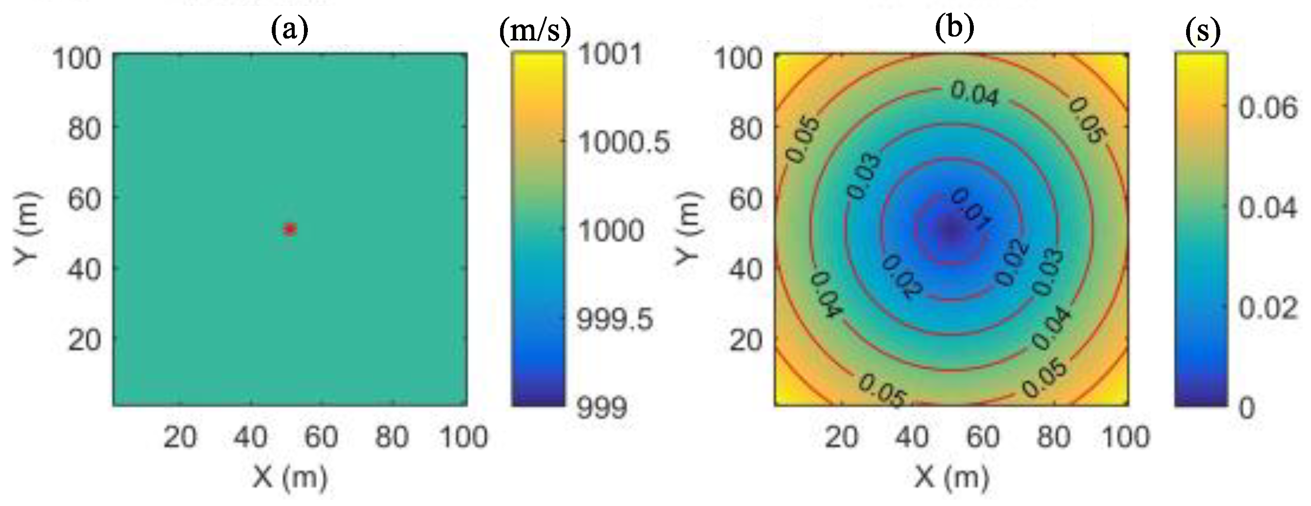
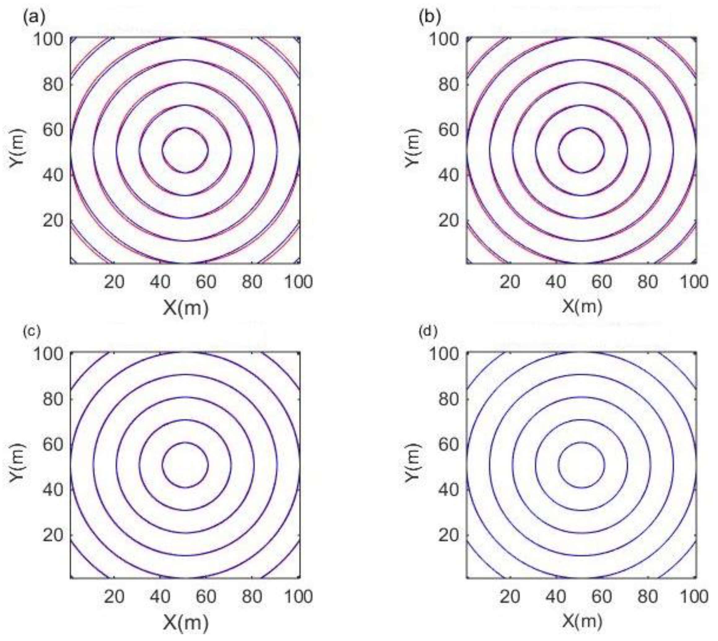
The homogeneous model is shown in Figure 4. The number of grids is 100 × 100. The vertical and horizontal grid spacing is 10 m, and the source point position is (51). The theoretical value $T_a$ of the travel time at each grid node is

$$T_a=\sqrt{{\left(x-x_0\right)}^2+{\left(y-y_0\right)}^2}$$

(20)

where $\left(x_0,y_0\right)$ is the coordinate of the source, and Figure 4b is the theoretical travel time contour of the homogeneous model.

Figure 5 shows a comparison between the theoretical travel time and the calculated travel time of FMM and MSFM. The red line represents the theoretical travel time and the blue line represents the calculated travel time. Figure 5a,c shows the first-order and second-order computational and theoretical travel time contours of the FMM algorithm, respectively. Figure 5b,d shows the first-order and second-order computational and theoretical travel time contours of the MSFM algorithm, respectively.

It can be seen from the graph that when the two algorithms offer the same first-order approximation or the same second-order approximation, the difference between the calculated value and the theoretical value of MSFM is smaller than that of FMM. In the case of the second-order approximation, the difference between the calculated value and the theoretical value of the two algorithms is obviously smaller than that of the first-order approximation. Among them, the travel time calculation value of the second-order MSFM almost coincides with its theoretical value, which shows that its calculation accuracy is the highest.

In order to compare the computational accuracy and efficiency of the two algorithms, two mesh spacings and three error indices are used to test the first-order and second-order of FMM and MSFM, respectively. The error indexes are as follows:

$$L_1=\frac{1}{n}{\displaystyle {\sum }_{i=1}^n\left|T-T_a\right|}$$

(21)

$$L_2=\frac{1}{n}{{\displaystyle {\sum }_{i=1}^n\left|T-T_a\right|}}^2$$

(22)

$$L_{\max }=\max \left(\left|T-T_a\right|\right)$$

(23)

where $T_a$ is the theoretical travel time, $T$ is the computational travel time, and $n$ is the total number of grid nodes.

Table 1. Computational accuracy and efficiency of FMM and MSFM.

Grids			100 × 100
Method/Error	L1	L2	Lmax	Time/seconds
FMM1	0.746	0.697	1.315	1.011
MSFM1	0.607	0.446	0.973	1.164
FMM2	0.197	0.042	0.329	1.054
MSFM2	0.040	0.003	0.188	1.288
Grids			500 × 500
Method/Error	L1	L2	Lmax	Time/seconds
FMM1	1.055	1.538	2.062	24.428
MSFM1	0.915	1.116	1.657	29.334
FMM2	0.175	0.035	0.329	26.674
MSFM2	0.049	0.004	0.188	32.638

lists the error and time-consuming data of the 2 m and 10 m grid spacing, the first-order FMM (FMM1), the second-order FMM (FMM2), the first-order MSFM (MSFM1), and the second-order MSFM (MSFM2). The data in the analysis table (Table 1) show that: From the perspective of calculation accuracy, the three kinds of errors in FMM and MSFM are very small, indicating a very high calculation accuracy. By observing the table data vertically, we can see that the error fluctuation of FMM and MSFM is small, demonstrating that both methods are relatively stable.

When the table data are observed longitudinally, it can be seen that FMM1 > MSFM1 > FMM2 > MSFM2. The error of the second-order difference format is smaller than that of the first-order difference format, which fully verifies that the MSFM algorithm has higher calculation accuracy.

From the perspective of computational efficiency, there are two main parts: the time-consuming calculation and the time-consuming operation. The MSFM algorithm requires two templates, while the FMM algorithm only needs to use one template for calculation. In theory, the MSFM algorithm should consume twice as much time as the FMM algorithm. However, the operations for inserting and removing the two algorithms in the narrow band are the same. Table 1 shows that the time-consuming ratio of the MSFM over FMM increases as the number of grids increases, which further verifies that the MSFM algorithm has higher computational efficiency.

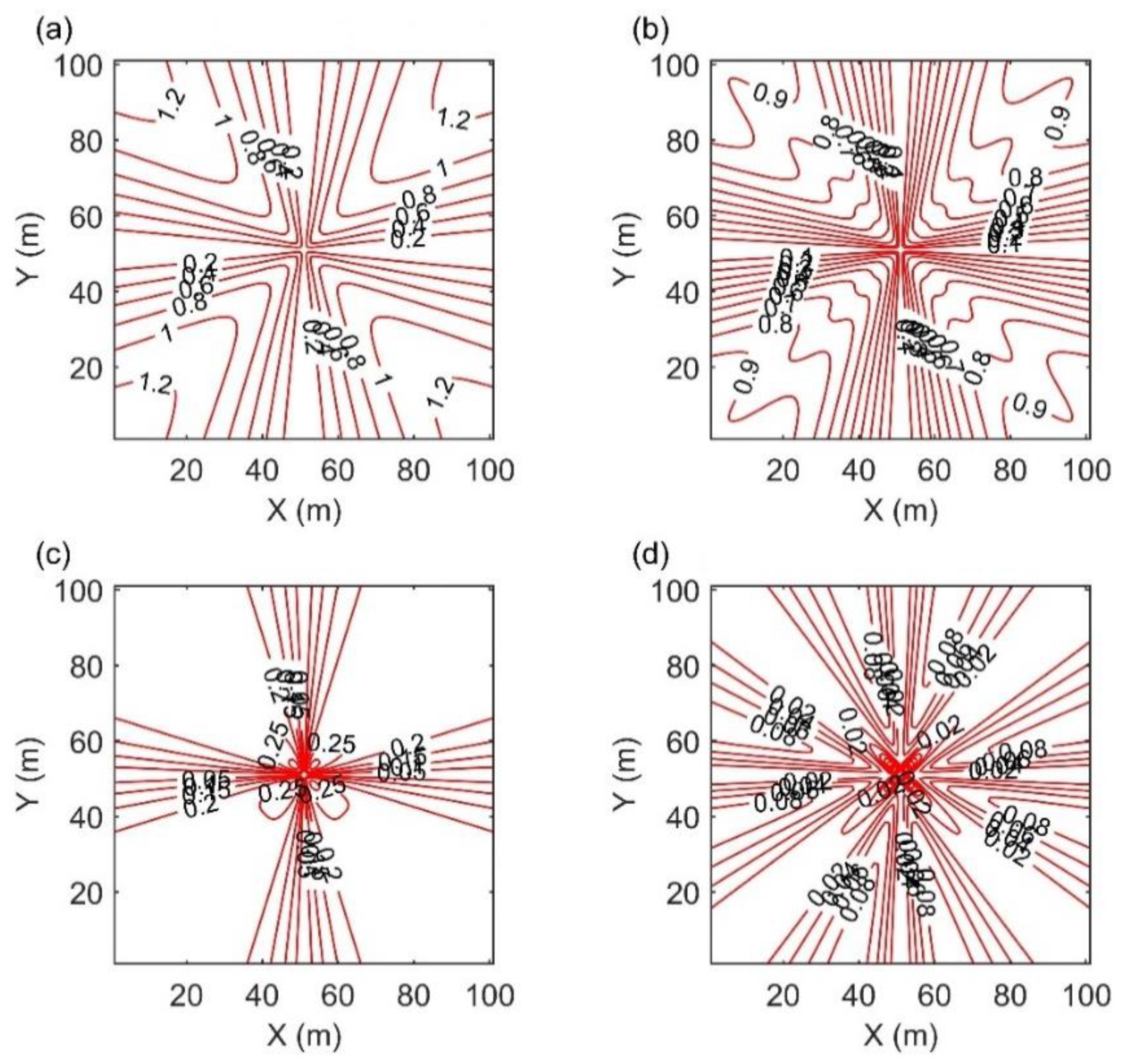
As can be seen from Figure 6, although the second-order format FMM improves calculation accuracy, the diagonal direction region error rapidly increases. The MSFM method improves the error of the FMM algorithm and improves its adaptability to complex models.

2.3. Inversion Methods

The theoretical basis of travel time tomography is the Radon transform. Assuming that $v(x,y)$ is a continuous velocity field, the travel time can be expressed as

$$t={\displaystyle \underset{L}{\int }s\left(x,y\right)dL}$$

(24)

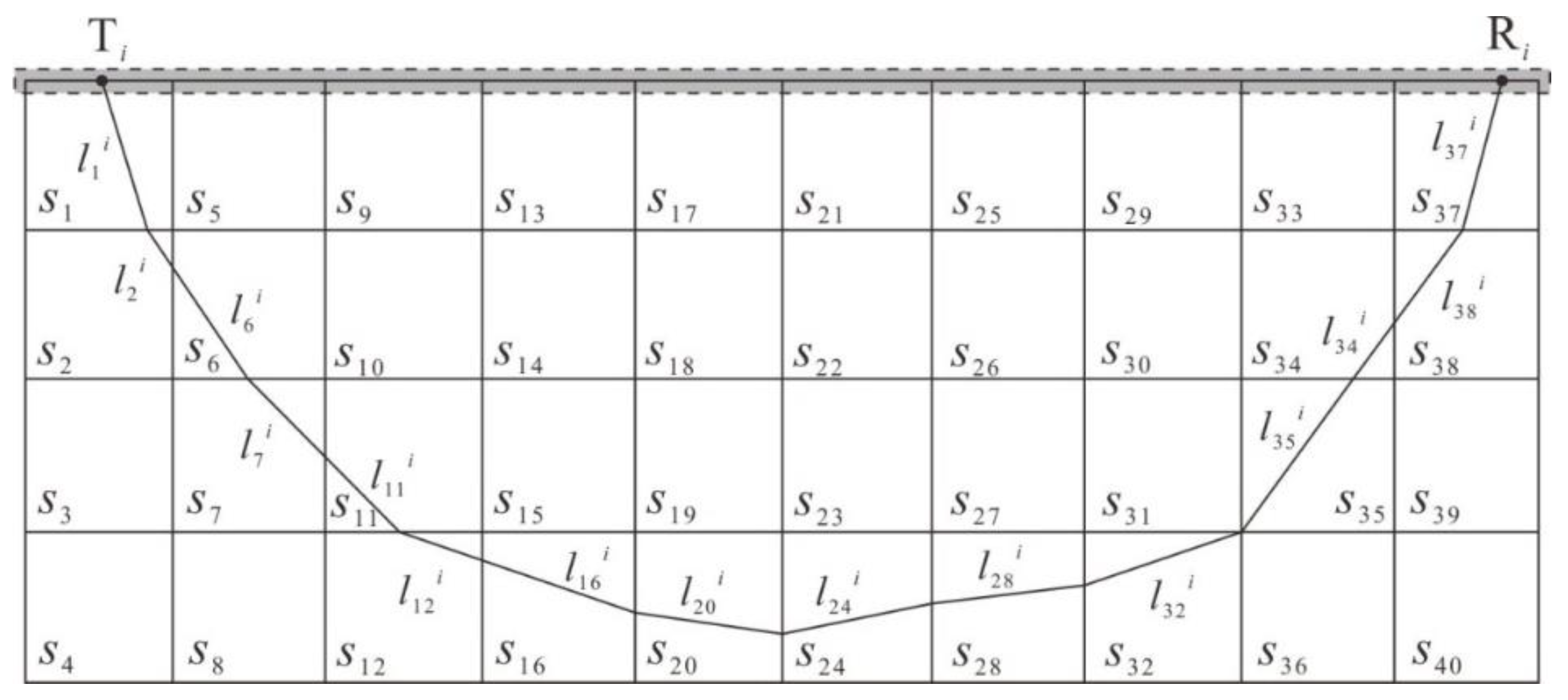
where $t$ is travel time, $s(x,y)=\frac{1}{v(x,y)}$ is the slowness field, and the integral path $L$ is the ray path from the source point to the receiving point. The first step in solving this problem is to discretize the slow field. In this way, Formula (25) can be obtained:

$$t_i={\displaystyle \sum _j{l}_j^i}{S}_j$$

(25)

where $i$ is the ith ray, $j$ is the jth discrete slowness grid, and $l$ is the length of the ray segment in each slowness grid. $l_j^i$ is the distance traveled by the ith ray in the jth grid, as shown in Figure 7.

Therefore, we can transform the nonlinear problem of travel time tomography into a linear problem. When there are $M$ rays passing through the region to be inverted, Equation (25) becomes a linear system of $M$ equations:

$$\left[\begin{array}{l}{t}_1\\ t_2\\ t_3\\ \dots \\ t_M\end{array}\right]=\left[\begin{array}{cccc}{L}_{10}& L_{11}& \dots \dots & L_{1N}\\ L_{20}& L_{21}& \dots \dots & L_{2N}\\ L_{30}& L_{31}& \dots \dots & L_{3N}\\ \begin{array}{l}\dots \\ L_{M0}\end{array}& \begin{array}{l}\dots \\ L_{M1}\end{array}& \begin{array}{l}\dots \dots \\ \dots \dots \end{array}& \begin{array}{l}\dots \\ L_{MN}\end{array}\end{array}\right]\left[\begin{array}{l}{s}_0\\ s_1\\ s_2\\ \dots \\ s_N\end{array}\right]$$

(26)

where $t_i(i=1,2,\dots ,M)$ is the travel time vector, $s_i(i=1,2,\dots ,N)$ is the slowness vector, and the distance matrix $L_{M\times N}$ is generally a large sparse matrix.

Then the Tikhonov regularization function [42] is introduced to transform the inversion problem into the minimum value problem for solving the following objective functions:

$$\mathsf{\Phi }(s)={\mathsf{\Phi }}_d(s)+{\lambda }^2{\mathsf{\Phi }}_m(s)$$

(27)

where ${\mathsf{\Phi }}_d(s)$ and ${\mathsf{\Phi }}_m(s)$ are the objective functions in the data space and the model space, respectively. λ is the regularization factor, which is used to adjust the weight between the data space ${\mathsf{\Phi }}_d(s)$ and the model space ${\mathsf{\Phi }}_m(s)$.

In the travel time tomography inversion of refracted waves, ${\mathsf{\Phi }}_d(s)$ can be expressed as follows:

$${\mathsf{\Phi }}_d(s)={\Vert W_d\left[t-d(s)\right]\Vert }^2=\frac{1}{2}{\displaystyle \sum _{i,j}^{N_d}\left[t_i-d_i(s)\right]}{W}_{ij}^d\left[t_j-d_j(s)\right]$$

(28)

Further, ${\mathsf{\Phi }}_m(s)$ can be expressed as follows:

$${\mathsf{\Phi }}_m(s)={\Vert W_m\left[s-s^0\right]\Vert }^2=\frac{1}{2}{\displaystyle \sum _{i,j}^{N_m}\left[s_i-s_i{}^0\right]}{W}_{ij}^m\left[s_j-s_j{}^0\right]$$

(29)

where $W_d$ and $W_m$ are the data weighting matrix and the model weighting matrix, respectively. $t$ and $d(s)$ are the observation travel time data and the calculation travel time data, respectively.

2.4. Combination of the Smallest Disturbance Constraint and the Smoothest Constraint

In order to reduce ill-posed and inversion multi-solution problems, we introduce the Tikhonov function with a priori information to solve the continuous medium inversion problem. The Tikhonov regularization function can be written as follows:

$$\mathsf{\Phi }(s)={\Vert W_d\left[t-d(s)\right]\Vert }^2+{\lambda }^2{\Vert W_m\left[s-s^0\right]\Vert }^2$$

(30)

Before inversion, three parameters need to be determined, the data weighting matrix $W_d$, the model weighting matrix $W_m$, and the regularization factor $\lambda$.

Generally, $W_d$ selects the $M\times M$-order unit matrix. In refraction travel time tomography, the observed travel time data are uniformly weighted.

The selection of $W_m$ is different. The commonly used regularization constraints can be divided into the following four types:

• Smallest model constraints: $W_m={\Vert m\Vert }^2$;
• Flattest constraints: $W_m={\Vert m^{\prime }\Vert }^2$, where $m^{\prime }$ is the first derivative of the model space;
• Smoothest constraints: $W_m={\Vert m^{″}\Vert }^2$, where $m^{″}$ is the second derivative of the model space;
• Smallest perturbation constraints: $W_m={\Vert m-\tilde{m}\Vert }^2$, where $\tilde{m}$ is a priori reference model;

In this paper, the results of the t0 difference method are used as an a priori slowness model for presumptive information. However, because of the limitations of the t0 difference method, we will adopt the composite constraint method, which combines the smallest perturbation constraints and the smoothest constraints. This method not only guarantees the uniqueness and rationality of the solution but also guarantees the stability and convergence of the solution.

2.5. Dynamic Selection of Regularization Factor

The regularization factor $\lambda$ determines the relative weight relationship between the data space and the model space in the objective function. When $\lambda$ trends toward zero, the fitting degree of the data is better, but the model is rougher. When $\lambda$ trends toward infinity, the fitting degree of the data is worse, but the model is smoother.

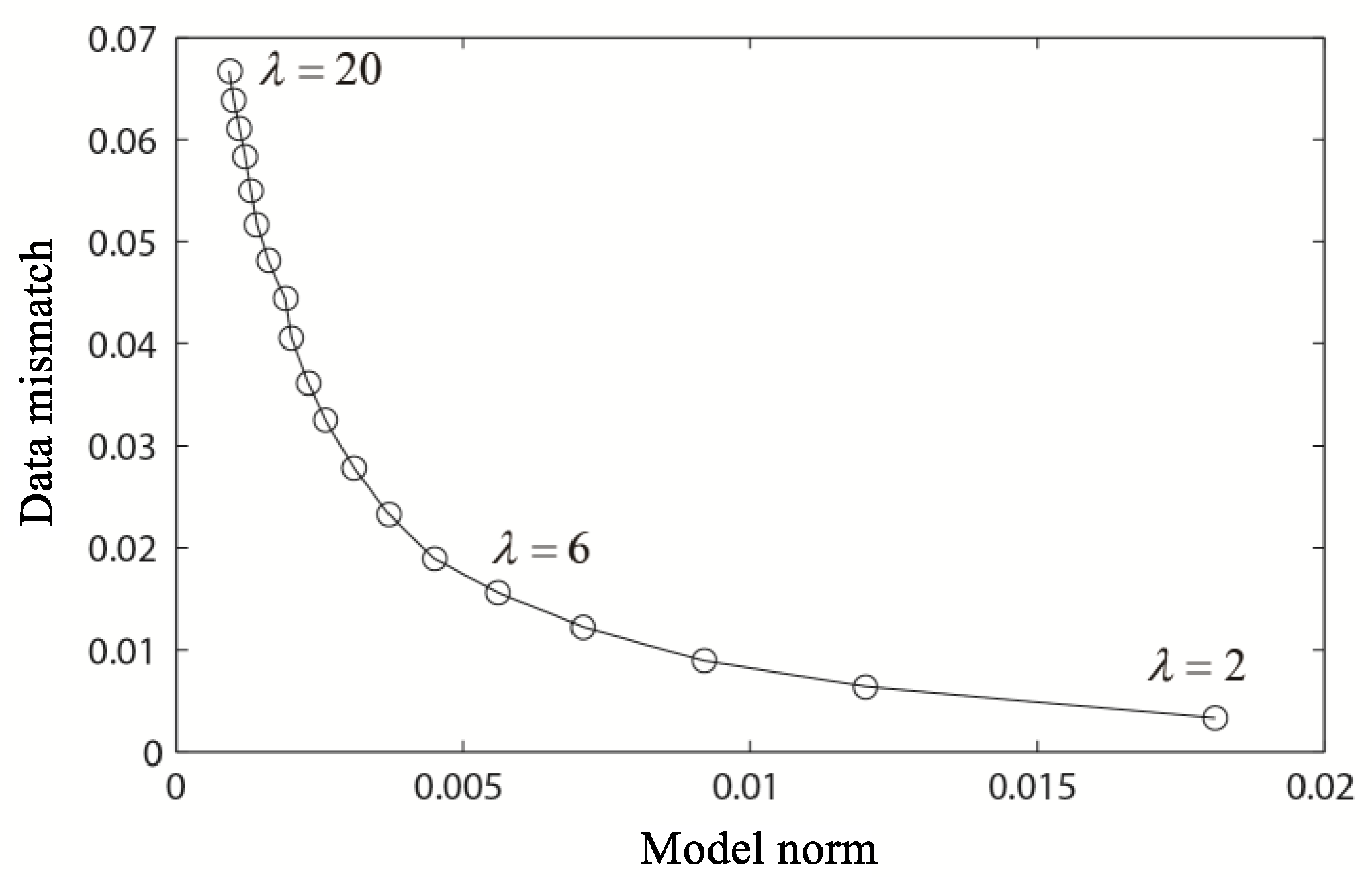
The method of selecting regularization factors is usually L-curve method, as shown in Figure 8.

This curve represents the relationship between data fitness and model fitness with different regularization factors. It requires many experiments to select $\lambda$ [14]. Generally, the regularization factor at the maximum curvature of the L-shaped curve is the optimal regularization factor [37]. As shown in Figure 8, $\lambda =6$ is the optimum solution.

Because the process of selecting the most regularization factors needs a large number of calculation experiments, this paper proposes an improved method for selecting regularization factors.

The value of the regularization factor represents the weight relationship between the degree of data fitting and the degree of model fitting. In order to improve the degree of data fitting and model fitting, we need to adjust the value of the regularization factor in the iterative process. According to the above reasons, this paper designs a method to select dynamic regularization factors.

In the iterative process, the large-scale shape of the model is outlined by using a larger regularization factor, and the inversion result is smoother at this time. Then the regularization factor is continuously reduced to accurately describe the disturbance of the small-scale slowness model, and the inversion result will be closer to the real model. This method not only ensures the convergence and stability of the inversion results, but also improves the fitting degree of the data.

Assuming that there is a simple linear relationship in the fitting difference between the data and the model and regularization factor λ, we can select the next λ according to the variation of the fitting difference of each iteration inversion. λ decreases with the decrease of data fitting difference. So, regularization factor λ can be selected dynamically.

3. Fault Model Inversion

We will select a representative and geologically reasonable near surface velocity model to test the feasibility and reliability of the improved travel time tomographic inversion algorithm proposed in this paper. The synthetic data is a three-layer fault model. The selection of algorithms and parameters are as follows:

• The maximum signal-to-noise ratio method is used for the first arrival travel time extraction.
• A second-order MSFM method with the highest accuracy is used for the forward travel time calculation.
• Selecting the unit matrix as the data weighting matrix.
• The weighted matrix of the model chooses a composite constraint matrix, which combines the second-order differential Laplacian with the prior information model obtained by the t0 difference method.
• The dynamic change of regularization factor selection with the iteration process.
• Sparse linear equations and least square problems (LSQRs) with the highest efficiency and stability for solving a large sparse matrix.
• The number of iterations is 10.

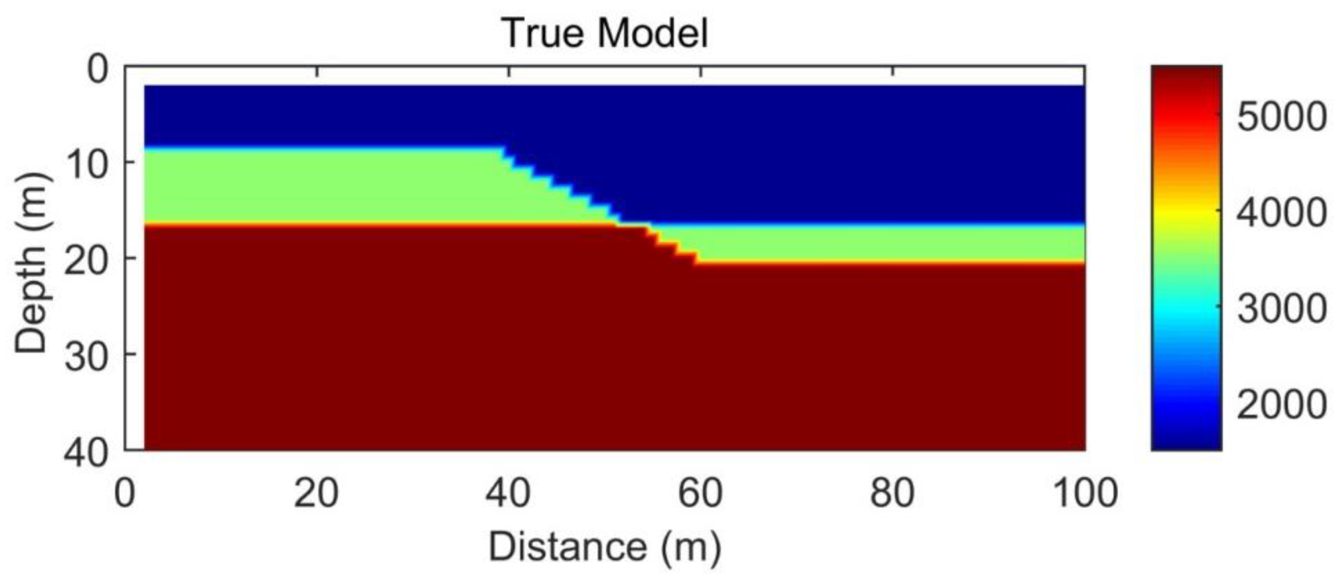
The fault model is shown in Figure 9. The lateral distance is 100 m, and the vertical depth is 40 m. There is a steep inclined reverse fault interface between 40 m and 60 m. The interface depth of the first refractive layer increases from 8 m to 16 m, and the interface depth of the second refractive layer increases from 16 m to 20 m. The first layer has a speed of 1500 m/s, the second layer has a speed of 3500 m/s, and the third layer has a speed of 5500 m/s. The size of the grid is 1 m. The observation system refers to shooting and receiving conditions on the surface. The offset distance is 4 m, the shot spacing is 2 m, and the trace spacing is 1 meter. A total of 49 seismic sources and 97 receivers are used.

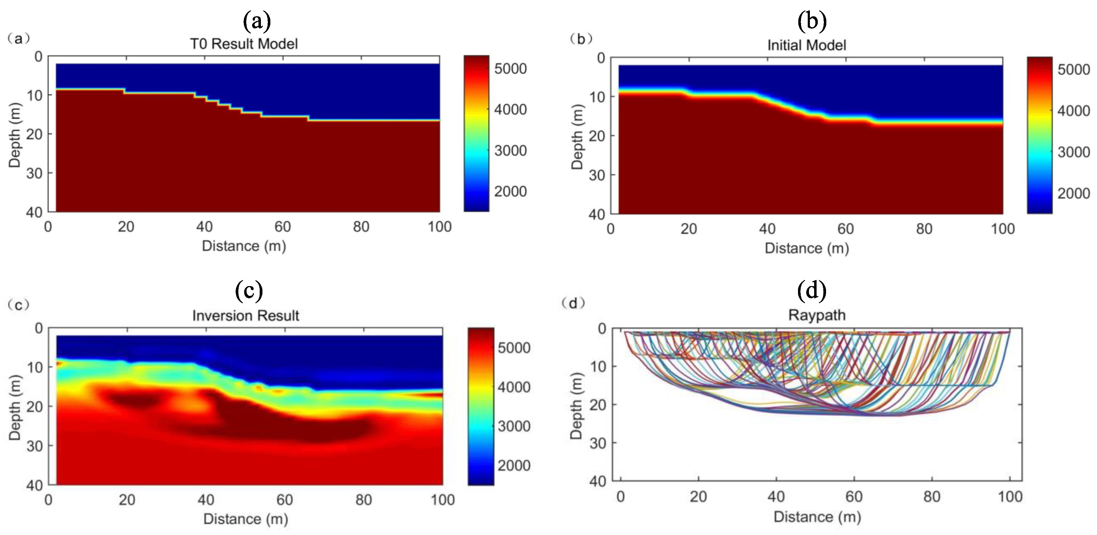
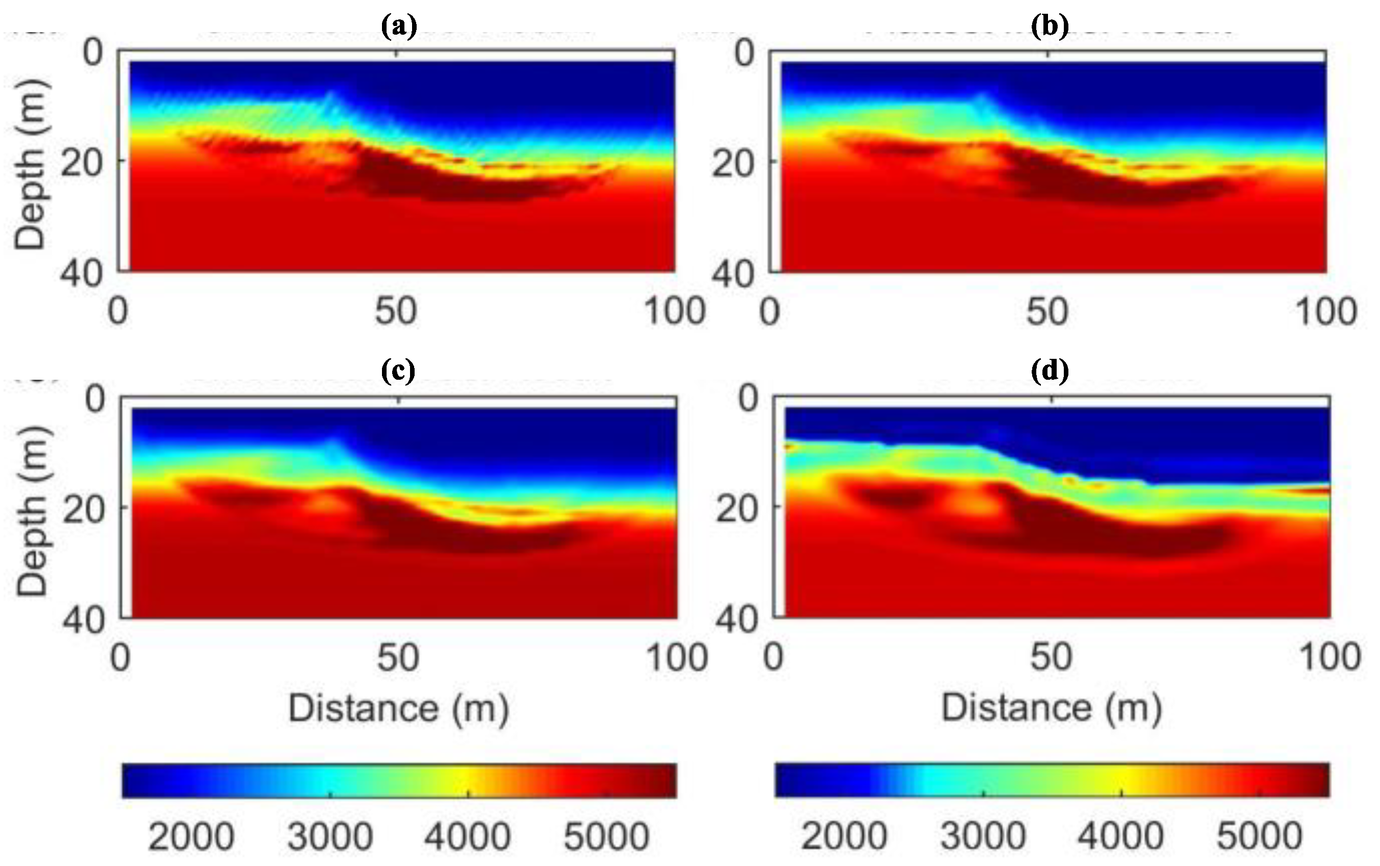
Figure 10a is a preliminary interpretation result of the t0 difference method for a real model. In order to avoid the local extremum in the inversion process, Figure 10b is obtained by an inverse distance gradient weighted interpolation of the interval velocity on the interface of the velocity mutation from the t0 difference method. Then, the model is used as an a priori model in the inversion process. Figure 10c is the inversion result. 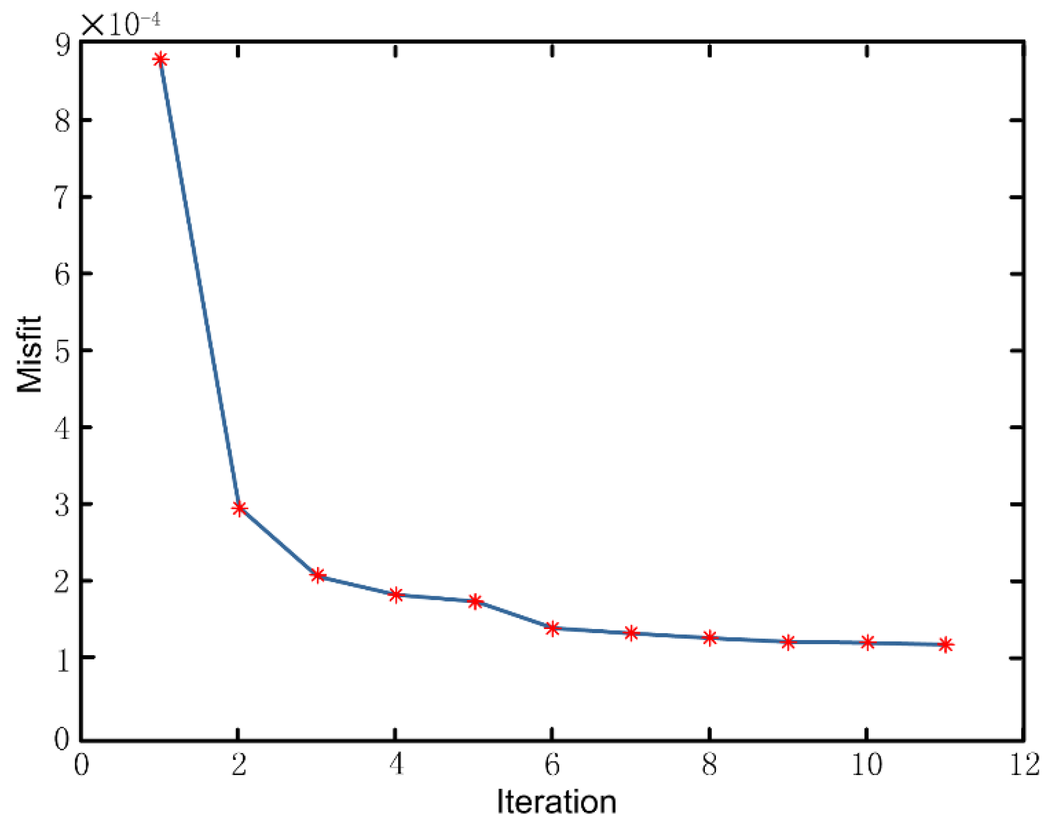Figure 10d is the corresponding ray path and Figure 11 is the fitting curve of the inversion iteration error. The error curve is used to evaluate the applicability of the model.

From the inversion results, the layered morphology fitting is very accurate, and the velocity values of each layer are also consistent with those of the real model. Errors mainly occur at the interface of the fault location, and the inversion results show a smooth effect. Steep faults become gentle, which is one of the characteristics of refraction travel time tomography. In addition, the uncertainty of the depth and velocity of the stratum interface increases towards the edge of the model, which is caused by insufficient ray coverage at the edge of the model. From the ray path, the ray tends to gather at the high-speed area and basically glide along the high-speed interface. It can be seen that the depth of the three-layer interface depicted is more accurate. From the error fitting curve, after 10 iterations, the root mean square error converges quickly and drops to a very small level, which shows that the data fitting is very good. In general, the three-layer fault structure has been reconstructed well, which verifies the effectiveness and reliability of the algorithm.

4. Inversion Effect Analysis

We next verify the reliability and effectiveness of the algorithm proposed in this paper and then discuss the differences before and after optimization. This study mainly analyzes the inversion effect from the forward travel time calculation method and the constraint method in the iterative inversion process.

4.1. Effect of Forward Travel Time Algorithms

We present two forward travel time calculation methods, FMM and MSFM. In this section, we will compare the inversion effects of these two algorithms in a fault model. In order to control the variables, we set the default constraint method as the dynamic prior model composite constraints (DPMCC) and selected an efficient and stable LSQRs algorithm for linear inversion. Both methods use the t0 difference method to obtain the priori model. The offset distance is 4 m, the shot spacing is 2 m, and the trace spacing is 1 meter. A total of 49 seismic sources and 97 receivers are used.

Figure 12a is the inversion result of the FMM algorithm, and Figure 12b is the inversion result of the MSFM algorithm. We can see from the figure that when FMM is used as the forward travel time calculation method, there are more false anomalies in the reconstructed velocity field, which are mainly concentrated near the fault.

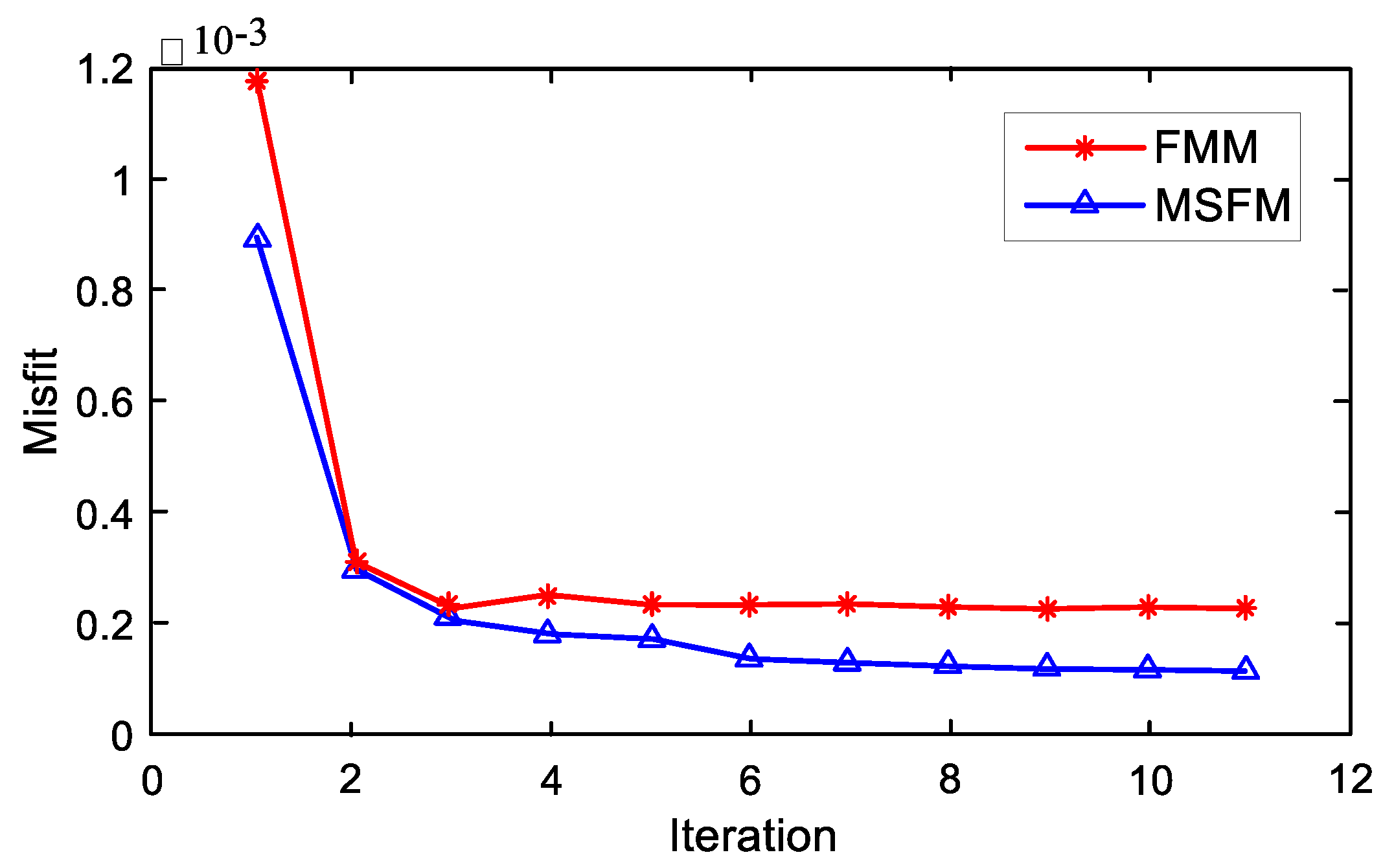
As shown in Figure 13, the effect of MSFM is better than that of FMM when the number of iterations is the same. In summary, the MSFM proposed in this paper is a better choice for tomography forward calculations.

4.2. Effect of the Constraint Method

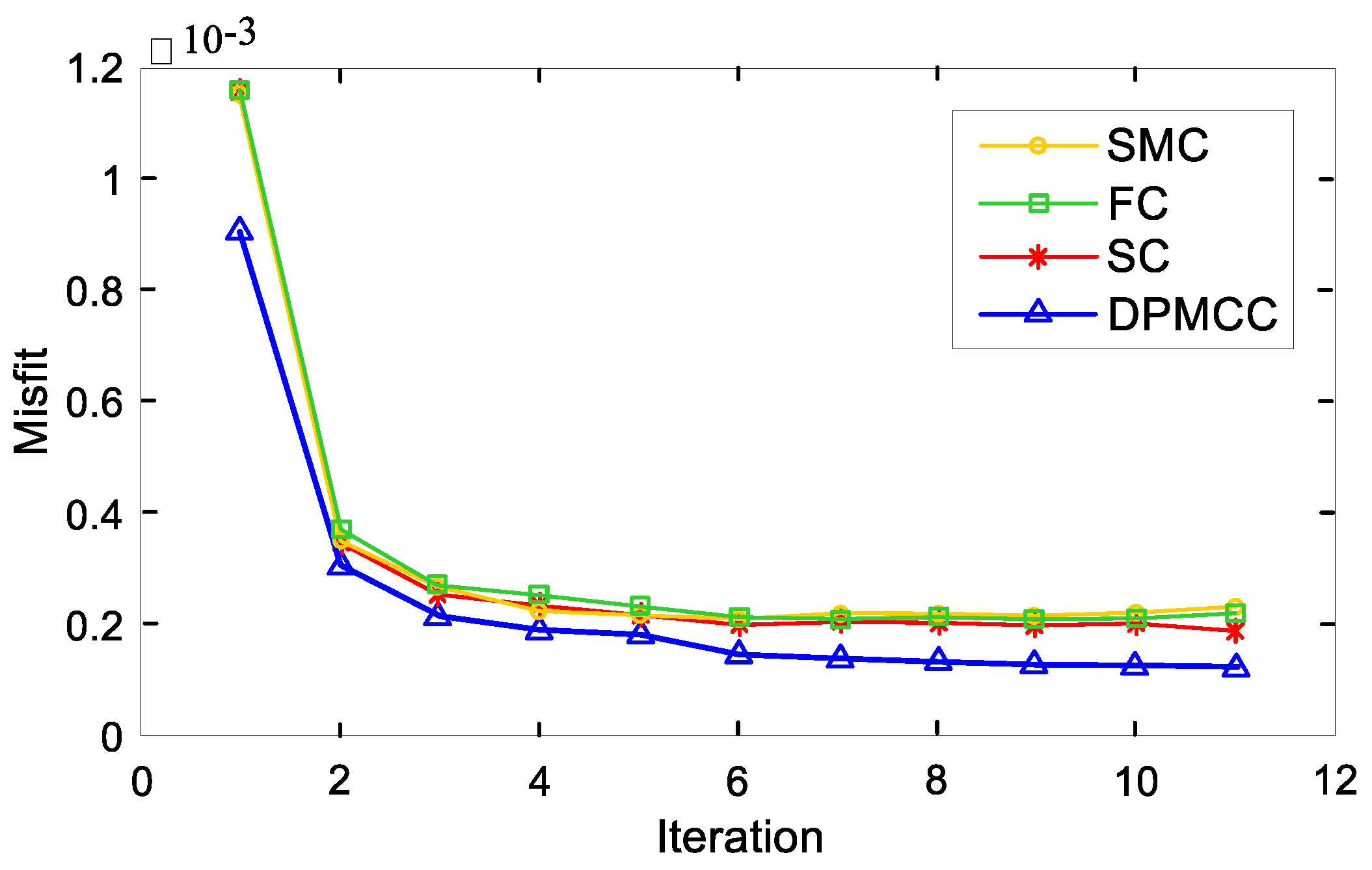
Four inversion regularization constraints are presented: smallest model constraints (SMC), flattest constraints (FC), smoothest constraints (SC), and dynamic prior model composite constraint (DPMCC). The dynamic prior model composite constraint use the t0 difference method to obtain the a priori model. The parameters of the four methods are the same. Offset distance is 4 m, shot spacing is 2 m. Trace spacing is 1 meter. A total of 49 seismic sources and 97 receivers are used.

In this section, we will compare the constraints of these four constraints in the travel time tomography inversion of the fault model. In order to control the variables, we set the default forward travel time method as MSFM, with its higher accuracy and efficiency. The LSQRs algorithm was chosen for solving a large sparse matrix.

As is shown in Figure 14a, there are many false anomalies and the boundaries of the layers are not clear enough. Figure 14b,c are both in better smoothness than that of Figure 14a. The inversion result of the algorithm we proposed is shown in Figure 14d. It can be seen that the interface of the layer is most clearly depicted, and there are few false anomalies. The inversion speed is closer to the real value, so its stability and convergence are the best.

As shown in Figure 15, when the number of iterations is the same, the constraint method proposed in this paper has the best effect. Therefore, DPMCC is a more effective method for inversion calculation.

5. Results

The refraction exploration data collected in this paper are from the highway tunnel exploration project, which is located in Northeast China. The purpose of this project is to determine the weak weathering interface at the entrance of the tunnel and reduce the potential risk of the exit as the entrance of the tunnel. The geological composition of the area is as follows: the surface layer is quaternary system, the lower part is bedrock, and the bedrock is not exposed in the area. The inclination of the ground is about 15°. Data acquisition was carried out using the seismic refraction method and an S-Land seismograph produced in the United States. Field measurement was carried out by hammering the source, which met the requirement of an interchange time difference less than 5 milliseconds. The length of the measuring line was about 240 m, the sampling rate was 0.5 milliseconds, the sampling time was 512 milliseconds, and the source spacing was 60 m with 5 sources; each source had 24 seismic receivers, and the trace spacing was 10 m.

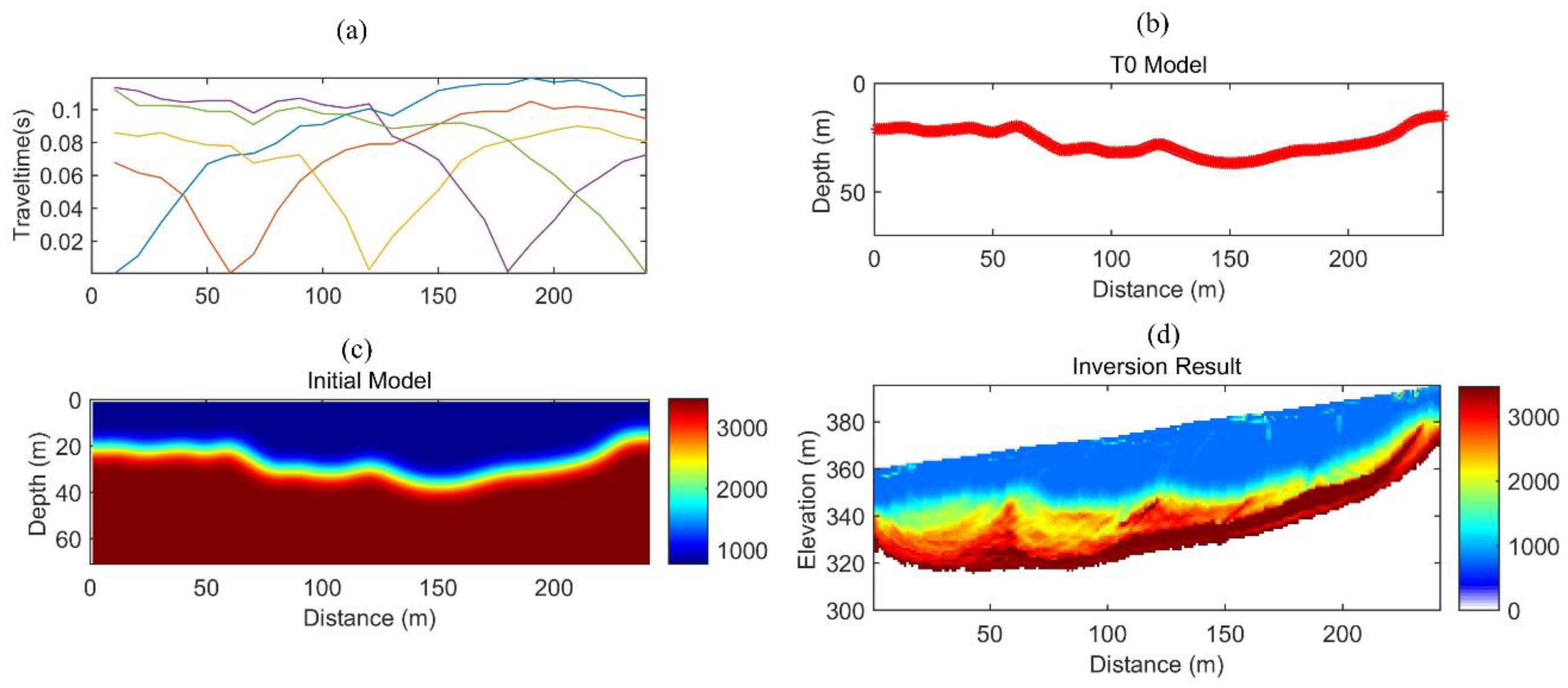
In the first step, we picked up the first arrival wave, as shown in Figure 16a. According to the far-shot travel time data, the t0 difference method is used for preliminary interpretation, and the basic formation interface results are obtained, as shown in Figure 16b. Then, the inverse distance gradient weighted interpolation of the velocity interface between the layers is carried out, and the model of Figure 16c is obtained. Finally, after the inversion calculation, the elevation data is introduced to get the results, as shown in Figure 16d.

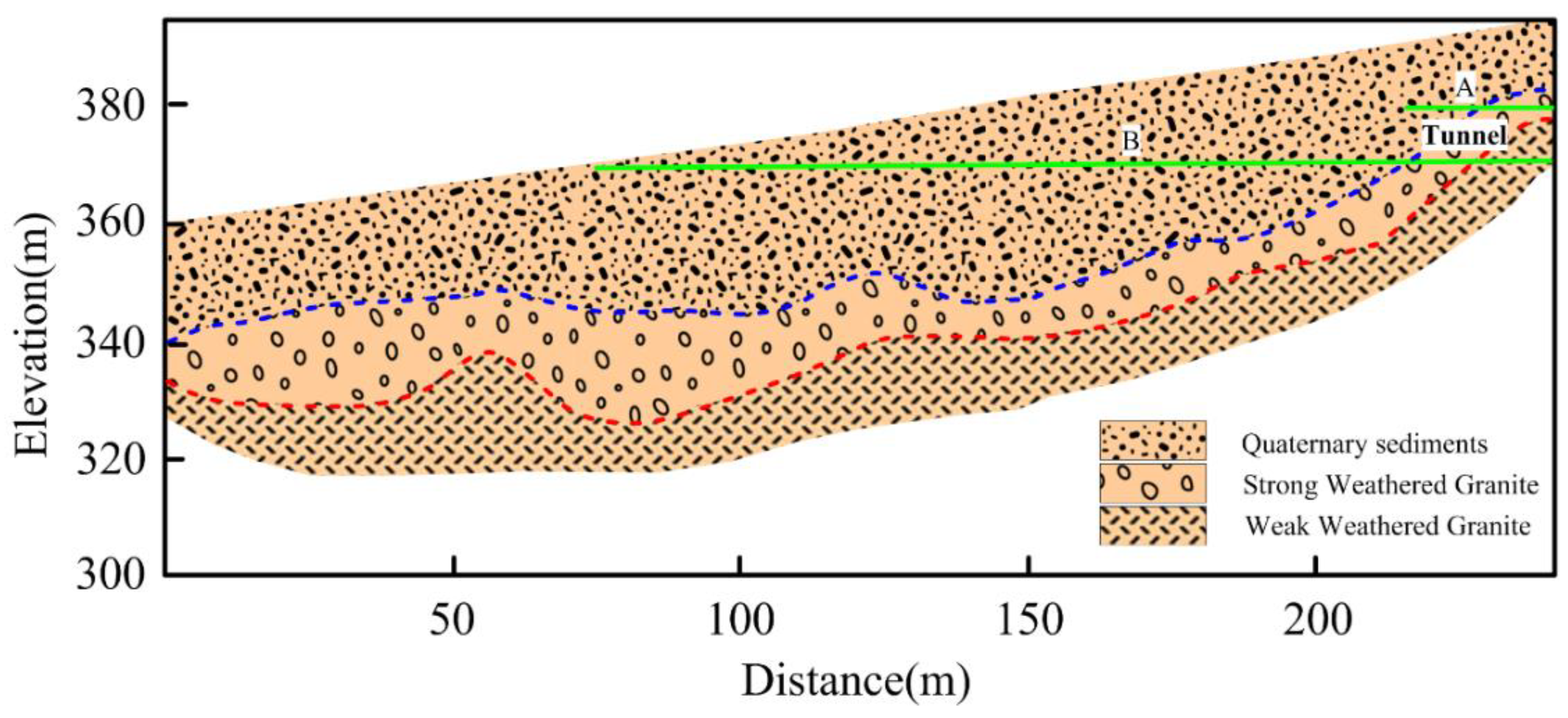
The elevation line and geological interpretation map of the tunnel are shown in Figure 17. The green line represents the upper and lower interfaces of the tunnel. According to the inversion results and geological data, the velocity range of the first layer, which is quaternary sediment, is 400–600 m/s. The low velocity layer is very obvious. Generally, the P-wave velocity of quaternary sediments is generally between 200–800 m/s. The depth of quaternary sediments is about 20–25 m. The velocity interface of the second layer, which is supposed to be strong weathered Granite, is about 1000–2500 m/s, and the lowest layer, which is supposed to be weak weathered Granite, is greater than 3000 m/s. The change rate of P-wave velocity of strong weathered granite is relatively large. The P-wave velocity of weak weathered granite is relatively high. In conclusion, according to the inversion results, the stratigraphic structure can be effectively divided.

The entrance of the tunnel in 230 m in the horizontal direction. It can be seen from Figure 15 that the top of the entrance is near the interface between the quaternary sediments and strong weathered granite. Therefore, attention should be paid to the construction in those areas. The types of lithology have guiding significance for tunnel excavation. According to the actual situation, it is a better choice for tunnel excavation to avoid a low-speed zone of strong weathering and select a hard and complete high-speed zone of rock. Thus, this method has guiding significance for tunnel engineering, can reduce the blindness of construction, and has the potential to improve the safety and reliability of tunnel engineering. The exploration of the seismic refraction method is limited by the site conditions, and the geological situation of the whole tunnel can be understood through very little exploration work. This method is fast and accurate, and is the first choice of shallow geological investigation work such as highway route investigation and hidden danger detection.

6. Conclusions

Refraction travel time tomography is not affected by the characteristics of the source and receiver, and its computational efficiency is much higher than the full waveform inversion method. Therefore, refraction travel time tomography is widely used in practical production and application. In this paper, the traditional travel time tomography method is optimized. First, we use MSFM instead of FMM as a forward algorithm. In the process of inversion calculation, dynamic selection of regularization factor and a constraint method based on a combination of the minimum perturbation constraints and smoothest constraints for the t0 difference method are proposed. By testing the synthetic data model, we proved the effectiveness and reliability of the improved travel time tomography method proposed in this paper. Through these efforts, we have come to some conclusions.

The t0 difference method was selected for the model test. This method can accurately calculate the depth of the layer interface and the average velocity of each layer. It can be used as a prior constraint in the inversion process of refraction travel time tomography.

The forward simulation shows that MSFM is superior to FMM in calculation accuracy, calculation efficiency, and adaptability to complex models. In the inversion, when FMM is used as a forward travel time calculation method, the reconstructed inversion results have more false anomalies, and FMM’s convergence speed and error are not as good as those of MSFM. Therefore, MSFM should be selected as the forward algorithm for refraction travel time tomography.

Because refraction travel time tomography is a mixed problem, regularization is needed to reduce the multiplicity of inversion solutions and improve the stability of these solutions. After synthesizing the advantages and disadvantages of several constraint methods, a composite constraint combines the minimum disturbance constraint and the smoothest constraint is proposed. By comparing the inversion results, it is found that the algorithm proposed in this paper has the least false anomalies and the best inversion effect. In the selection of regularization factors, this paper proposes a dynamic regularization factor method. In the iterative process, the large regularization factor is firstly used to outline the large-scale shape of the model, and then the regularization factor is continuously reduced to describe the disturbance of the small-scale slowness model.

Finally, the algorithm proposed in this paper was applied to the measured data. The refraction exploration data collected in this paper were taken from the highway tunnel exploration project, which is located in Northeast China. The depth of the bedrock can be inferred from the inversion results and is of guiding significance in tunnel excavation. According to the actual situation, it is a better choice for tunnel excavation to avoid highly weathered low-speed zones and instead select hard and complete rock high-speed zones. This could reduce the blindness of the construction and improve the safety and reliability of tunnel engineering. At the same time, we proved that the algorithm proposed in this paper is very practical.