1. Introduction
According to the Korean National Police Agency and the National Highway Traffic Safety Administration (NHTSA), the increase of vehicles on roads is accompanied by a proportional increase in traffic accidents caused by careless driving [
1,
2]. Several research and development projects are being conducted on functions such as advanced driver assistance systems (ADAS) around the world to improve drivers’ safety and convenience [
3]. The autonomous emergency braking (AEB) system is one such representative system. An AEB system analyzes the collision risk with the preceding vehicle and prevents or avoids a head-on collision, which can occur due to the driver’s carelessness, by operating the automatic control function at a dangerous moment [
4].
The existing AEB systems usually detect collision risks using obstacle detection sensors, such as cameras, light detection and ranging (LiDAR), and radio detecting and ranging (RADAR). As these sensors have limitations, many researchers have attempted to integrate multi-sensor data fusion technology with vehicle-to-vehicle (V2V) communication [
5]. In addition, existing AEB systems only cover limited road environments, such as curves with constant curvatures. The relative distance and the parameters of the AEB algorithm were calculated by the arc length of a certain sector based on the curvature and the angle between the two vehicles [
6,
7,
8]. Since the existing AEB systems do not consider the geometrical shape of winding roads, the relative distance is not very accurate.
Another study analyzed road alignments using a road section segmentation method. Straight sections account for approximately 34% and curve sections account for approximately 65% of all the roads in South Korea. Additionally, approximately 62% of the curve sections are reversed curves consisting of multiple curved radius and directions [
9]. Thus, the geometrical complexity of curves should be considered for the application of AEB systems to usual environments.
This study aims to improve the performance of an AEB system on curve roads. To achieve this aim, this study adopts V2V communication technology to overcome sensor limitations, such as blind spots. It also applies a curvilinear coordinate conversion, which is used for route planning of autonomous driving vehicle, to consider the geometrical complexity of curves [
10,
11]. Moreover, this study shows the effectiveness of the proposed AEB system in various curves in comparison with existing collision avoidance systems.
The remaining part of this paper proceeds as follows.
Section 2 explains the AEB system based on the curvilinear coordinate system. In
Section 3, a method for transforming the positions of the host and target vehicles is explained. Based on the curvilinear coordinate conversion, this method calculates the time-to-collision (TTC) required by the AEB system to perceive hazards. In
Section 4, a simulation is conducted for a curve with a constant curvature and a reversed curve, using the results of
Section 2 and
Section 3. Finally, the conclusions of this study are presented in
Section 5.
2. Curvilinear Coordinate Conversion
Most AEB system algorithms determine a collision risk by assuming a scenario for straight roads or a curve with a constant curvature. The relative distance is calculated by the arc length of a certain sector based on the curvature and the angle between the two vehicles [
6,
7,
8]. However, if the assumptions do not hold, the error is large in existing AEB systems. Accordingly, road alignment information is necessary to accurately determine the risk.
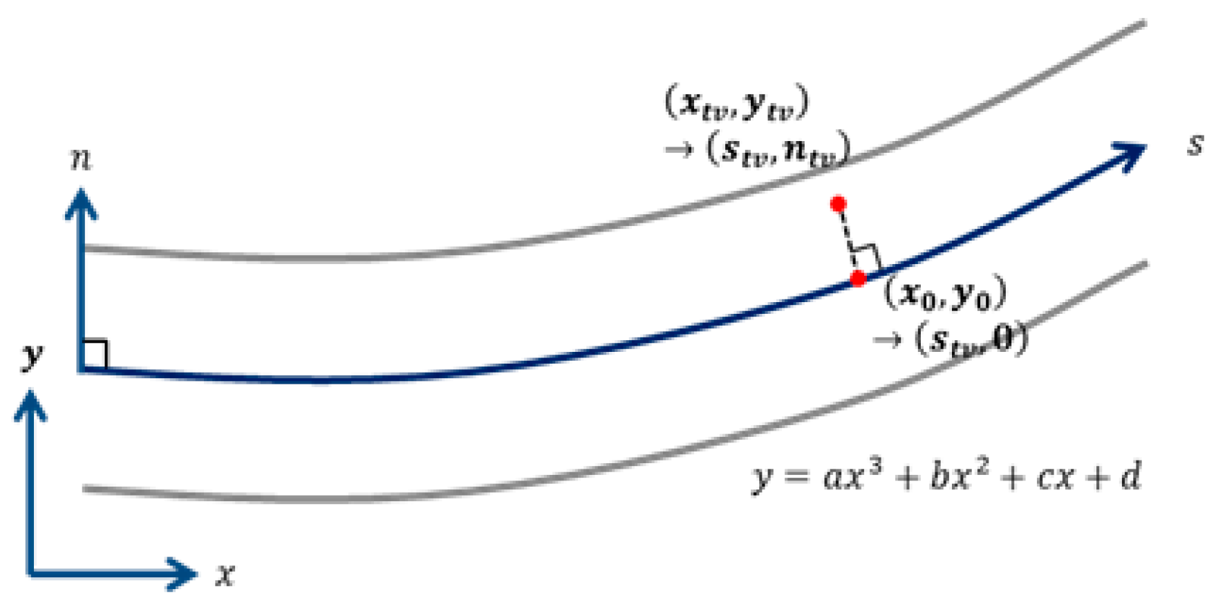
As the position and velocity data of the target vehicle are mostly obtained from sensors, they are expressed by a Cartesian coordinate system. However, it is difficult to calculate the relative distance reflecting geometric elements from the sensor information based on the Cartesian coordinate system. Thus, the curvilinear coordinate conversion is applied to solve this problem. Curvilinear coordinates express a transverse distance from a curved line by n and a longitudinal distance along a curved line by s. The curvilinear coordinate system enables a geometrical complexity to be expressed in an orthogonal coordinate system with orthogonality. Thus, the problem of estimating vehicle movement can be easily solved and the relative distance between vehicles, which includes geometric information, can be derived [
10,
11,
12].
Generally, a camera sensor provides road information through a third-degree polynomial in Equation (1). Therefore, it is assumed that road information is known by the third-degree polynomial.
As shown in
Figure 1, the position information of the target vehicle can be identified in the orthogonal coordinate system through a sensor. The curvilinear coordinate conversion consists of three main steps: finding the closest point to an equation of a curve, calculating a vertical distance n, and calculating an arc length s.
2.1. Finding the Closest Point to an Equation of a Curve
The essence of curvilinear coordinate conversion is to find the point on the curved road model closest to the vehicle. In this paper, this point is called the nearest point. That is, as shown in
Figure 1, the closest point
is the point where the vehicle and the curved road model meet vertically.
The closest point
is derived by using the distance D(x) between the target point
and the curve model. D(x) is calculated using Equation (2).
When D(x) has the lowest value, the vehicle and the curve road model are closest. The point where the derivative of D (x) is zero is calculated by Equation (3). At this time, D (x) has a maximum value or minimum value. In this paper, due to the geometrical characteristics of the road, there is always one minimum value, and the closest point
is calculated.
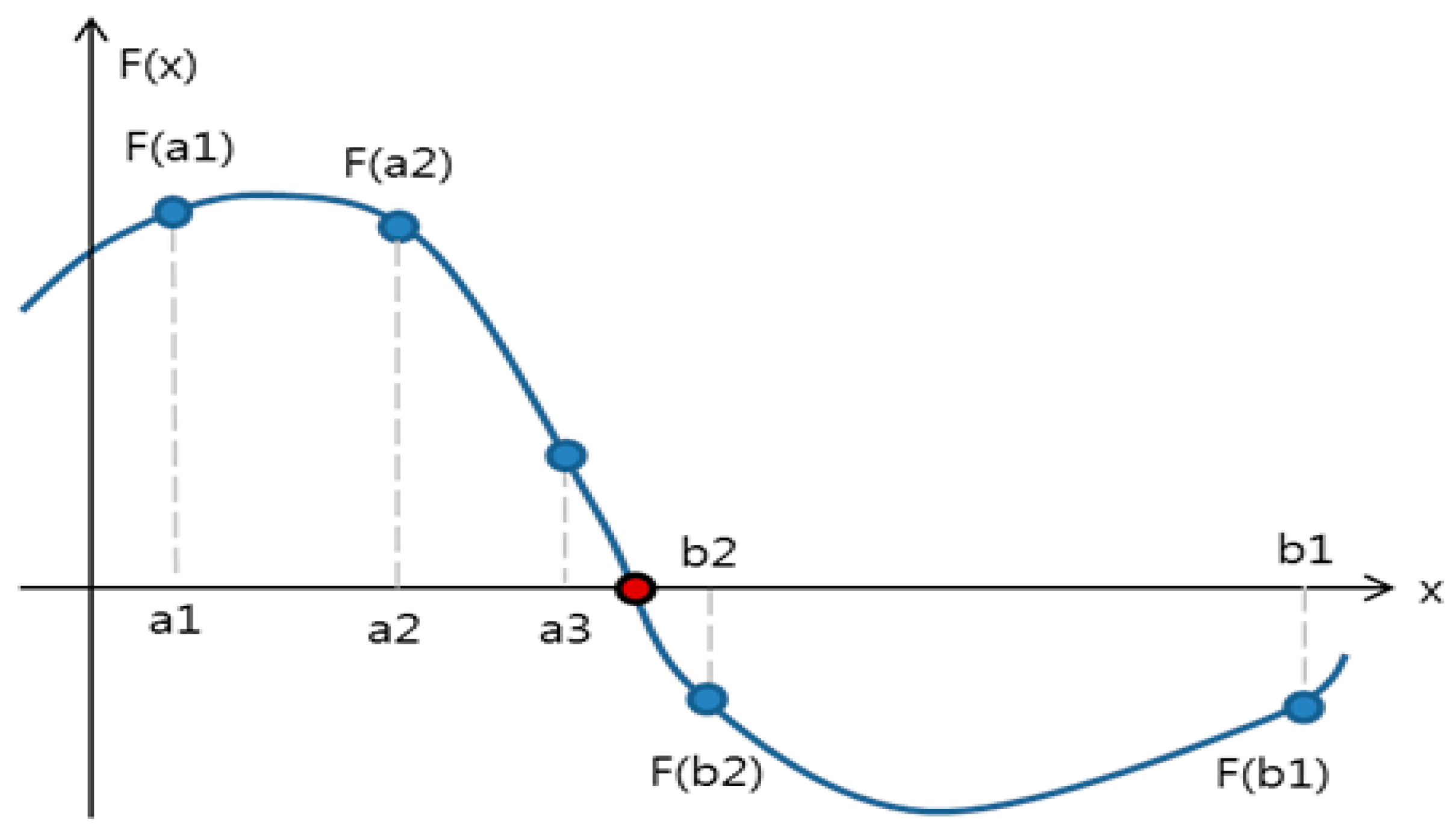
To find the root of Equation (3), existing studies employed various algorithms, such as the bisection method, the secant method, and Newton’s method. This study used the bisection method, which is the most representative algorithm, to obtain the solution. The bisection method is based on the intermediate value theorem, which states that the root can only be definitely found if an approximate position is given. The algorithm is simple, since iteration is utilized. As an approximate position of the root can be obtained from the global positioning system (GPS) data of the target vehicle, the bisection method can find the root quickly and accurately [
13].
Figure 2 and
Table 1 present the root-finding algorithm concept and pseudo code of the bisection method.
2.2. Calculation of Vertical Distance n
The vertical distance n is the distance between the closest point
and the target point
. As shown in Equation (4), n is calculated as the distance between a point and a line.
The vertical distance n is used to identify the lane of a vehicle. According to the Road Design Code of the Korean Ministry of Land, Transport, and Maritime Affairs, the minimum width of a lane should be 3.00 m for a speed limit of 60 km/h [
14]. Thus, as shown in Equation (5), if the vertical distance n is 1.50 m and below (i.e., does not exceed half of the minimum width), the target vehicle is running in the same lane. Otherwise, it can be judged to be running in a different lane.
This determines whether the AEB system operates or not.
2.3. Calculation of arc Length s
The arc length s is the distance from the initial position
to the closest point
[
15]. In Equation (6), it is used to calculate the relative distance between the host vehicle and the target vehicle.
3. AEB System Model
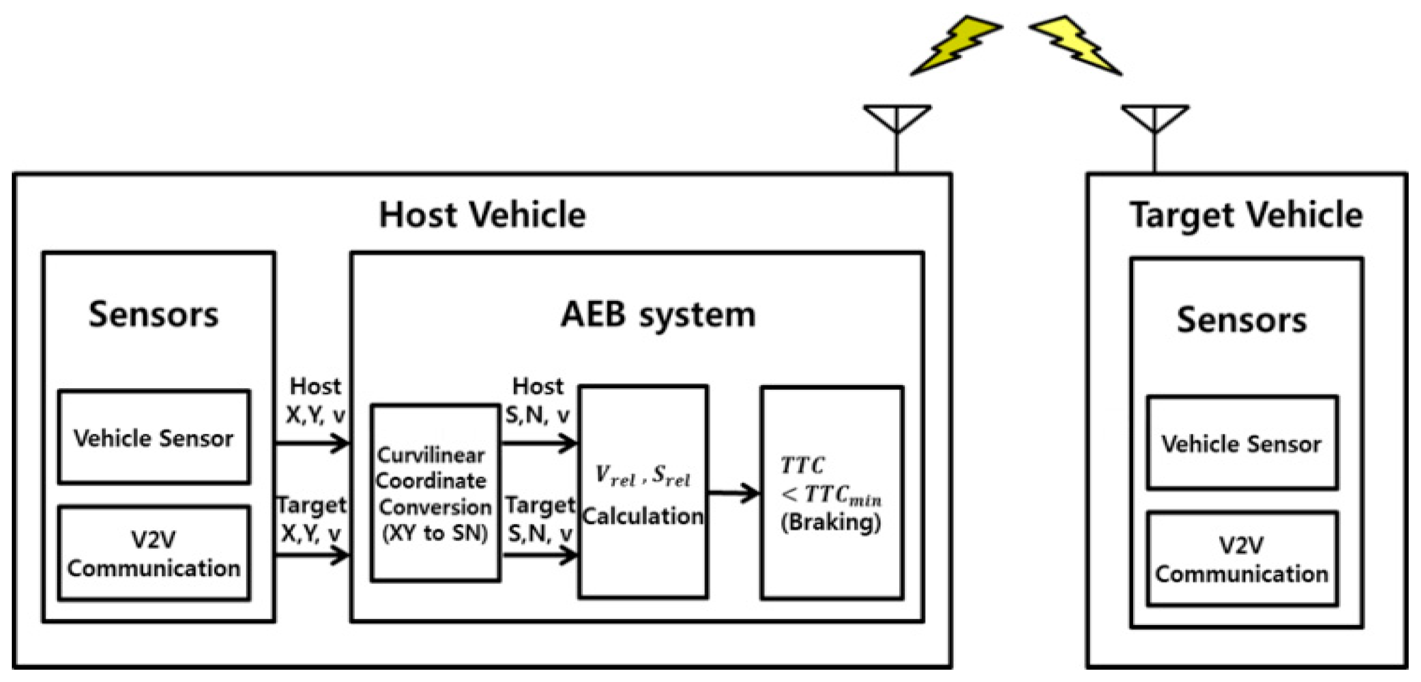
Figure 3 shows the overall configuration of the proposed AEB system based on the curvilinear coordinate system. This system consists of two main parts. The first part conveys data from velocity sensors and GPS sensors, which are installed in each vehicle, through V2V communication. The second part derives a relative distance between the host and target vehicles by converting the data of these vehicles to the curvilinear coordinate system and calculating TTC using the relative distance. Thus, a collision risk is calculated by reflecting the geometric road information.
The communication unit measures the velocity and acceleration of the host vehicle through in-vehicle sensors and the absolute position and azimuth angle of the host vehicle through the differential global positioning system (DGPS). In addition, the data of the target vehicle, including the absolute position, velocity, and acceleration, are obtained through V2V communication.
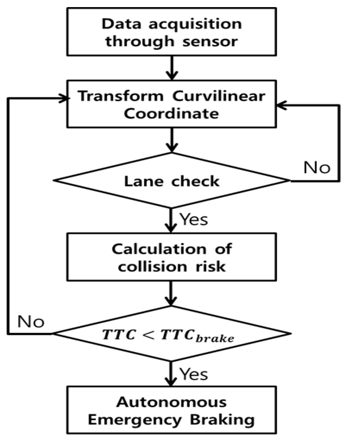
Figure 4 is a flow diagram of the risk determination algorithm for the proposed AEB system. The AEB system automatically engages the braking system based on a collision risk, which is calculated from the relative velocity and relative distance. The velocity and position data of the target vehicle are used to derive the relative velocity and distance [
4]. As the risk of a head-on collision needs to be considered for the operation of the AEB system, TTC was used as the risk indicator. Furthermore, V2V communication-based data was used to calculate TTC. Meanwhile, if the information of the target vehicle is obtained through V2V communication, the challenges related to limited sensing range and blind spots peculiar to sensors, including camera, RADAR, and LiDAR, can be solved.
The brake engagement time is determined by comparing TTC, which is the collision risk with the target vehicle, and
, which is the minimum brake engagement time for avoiding a collision. In other words, as expressed in Equation (7), the brake application time is considered to be the period when TTC becomes lower than
. At this time, the braking system is applied in the host vehicle.
The parameters of TTC and
for determining brake engagement time can be obtained using Equations (8) and (9). As the host vehicle is considered to be moving at a uniform speed until it is stopped by the braking system, the collision risk can be defined by using the formula of a uniformly accelerated motion [
16]. The minimum collision distance according to deceleration can be calculated using Equation (10). In Equation (9),
can be calculated using the velocity obtained from the minimum collision distance and V2V communication [
17].
As expressed in Equation (11), the relative distance
is calculated using the radius of a curve (R) and the angle between two vehicles (θ) in the existing paper [
6,
8].
The relative distance can only be accurately calculated using Equation (11) when the curvature is constant. Therefore, the arc length and vertical distance are needed to incorporate geometric factors of the curve. In this study, the arc length (s) and vertical distance (n) of the curve, including geometric elements of the curve, are derived from
Section 2. As shown in Equation (12), the relative distance is calculated as the distance formula between two points in the curvilinear coordinate system.
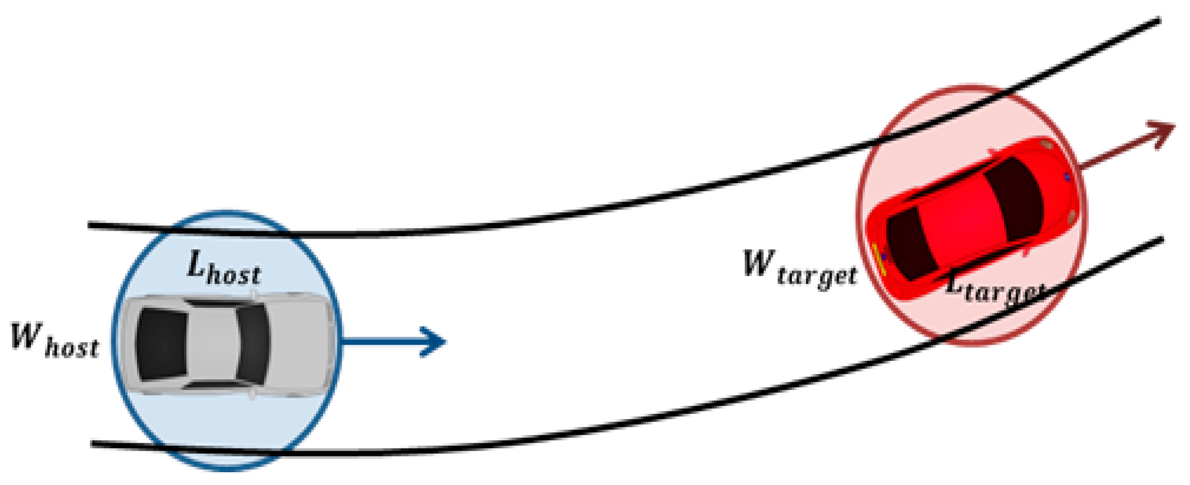
In addition, the positions corresponding to the gravity centers of each vehicle are obtained from the GPS sensors installed in each vehicle. Thus, the relative distance
to the target vehicle should reflect the size of the vehicle. As illustrated in
Figure 5, Equation (13) is derived by assuming vehicles to be circles [
6].
where s is the arc length, n is the vertical distance, L is the overall length of a vehicle, and W is the overall width of a vehicle.
The performance of the proposed AEB system was analyzed using the Mercedes Benz’s PRE-SAFE. It is a system intended to bridge the gap between primary safety, which aims to prevent a car from being involved in an accident, and secondary safety, which is the protection provided during a collision. At speeds above 30km/h, PRE-SAFE monitors the dynamic state of the vehicle (speed, rotation, etc.) and the driver’s inputs to steering, accelerator and brake, to determine whether or not emergency action is being taken.
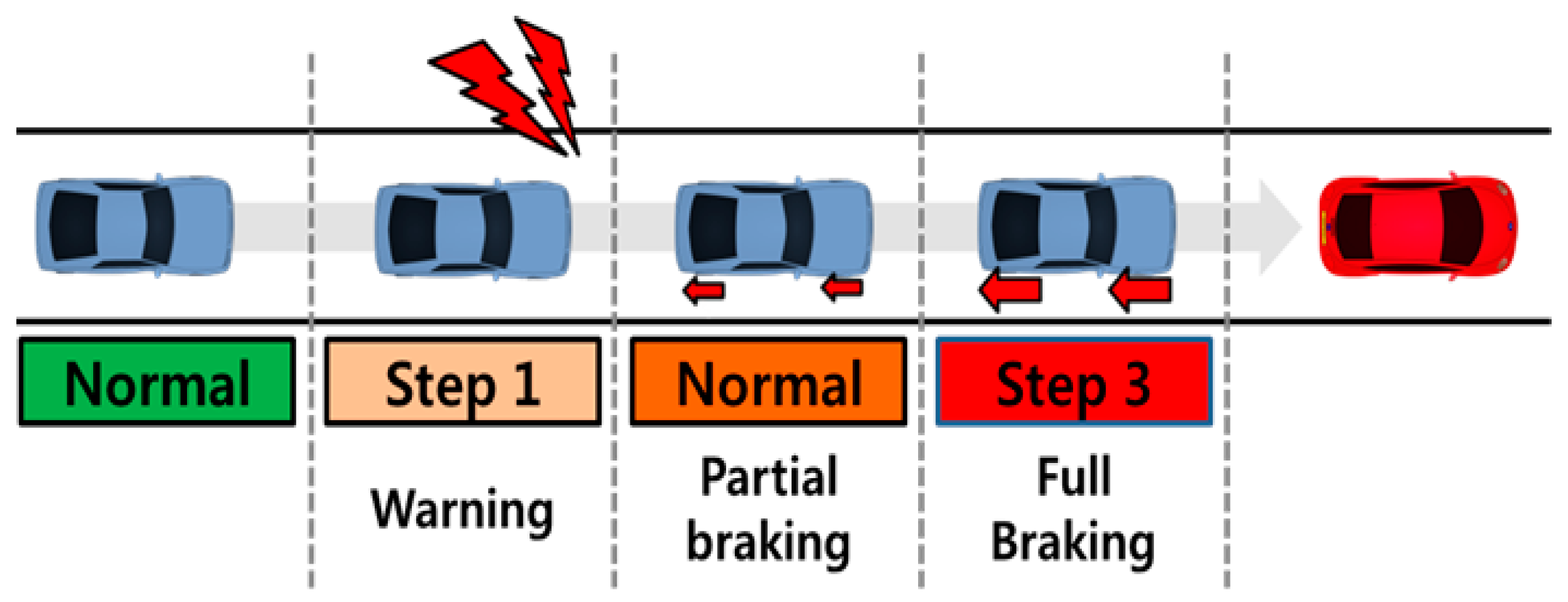
Figure 6 and
Table 2 present the detailed controls of the PRE-SAFE brake system that generates braking power based on TTC conditions. The PRE-SAFE brake strategy of Mercedes Benz consists of three steps. In step 1, TTC is 2.6 s and below, and a warning is issued to remind the driver of a dangerous situation. In step 2, TTC is 1.6 s and below, and partial braking is applied. In step 3, TTC is 0.6 s and below, and full braking is applied.
4. Simulation Scenarios and Results
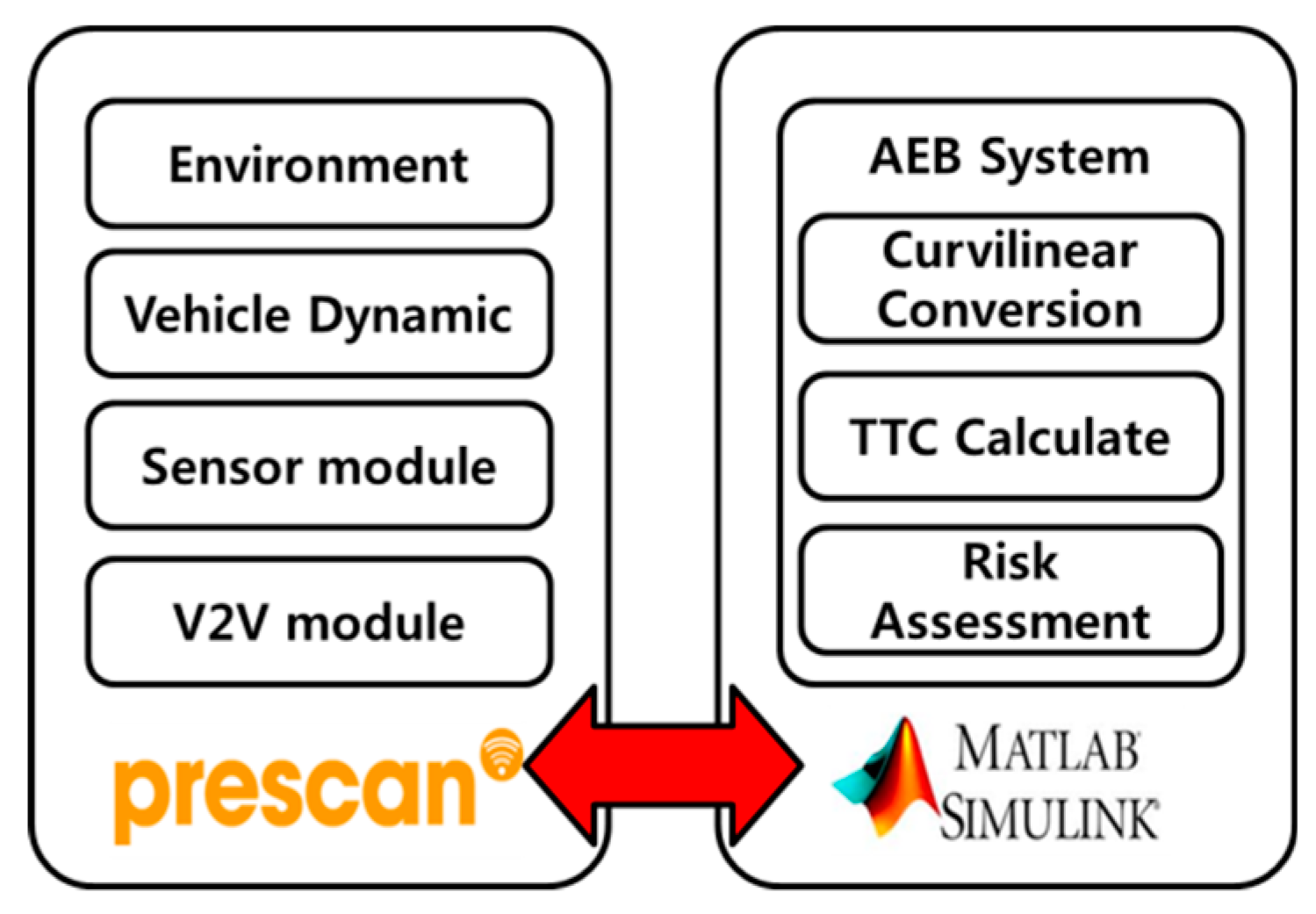
Figure 7 illustrates the simulated system configuration. PreScan was used to represent the basic environments of V2V communication and driving, while MATLAB/Simulink was used to implement the curvilinear coordinate conversion and risk judgment of the AEB system. The whole system was configured by linking PreScan and MATLAB/Simulink.
4.1. Simulation Scenarios
Two test scenarios were used to compare the performance differences between the proposed algorithms.
Figure 8 shows the simulation scenarios adopted in this study. First, the scenario for the conventional algorithm, which is a curve with a constant curvature, was used to compare the performance. Second, a scenario for a reversed curve was added. Based on a previous study that analyzed road alignments using a road section segmentation method, reversed curves consisting of different radii and directions accounted for approximately 70% of all curves, and approximately 62% of accidents occurred on reversed curves [
9]. This indicated that the AEB system had to be verified for reversed curves apart in addition to simple curves for practical applications.
In
Table 3, the driving scenarios and velocities of vehicles were set by referring to the AEB testing procedure of European New Car Assessment Programme (EuroNCAP) [
18]. The EuroNCAP is a European car safety performance assessment programme based in Leuven. On a curve, the host approaches the target vehicle at 60 km/h, while the target vehicle is stationary. Meanwhile, the AEB system operates through V2V communication.
The shapes of each road were determined based on the Road Design Code of the Ministry of Land, Transport, and Maritime Affairs. Each parameter was set by applying a minimum plane curve radius of 140 m and a minimum plane arc length of 70 m [
14].
4.2. Simulation Results
A curve with a constant curvature and a reversed curve were simulated to examine the performance of the curvilinear coordinate-based AEB system. The simulation results of the conventional AEB system and the proposed AEB system were compared for curves.
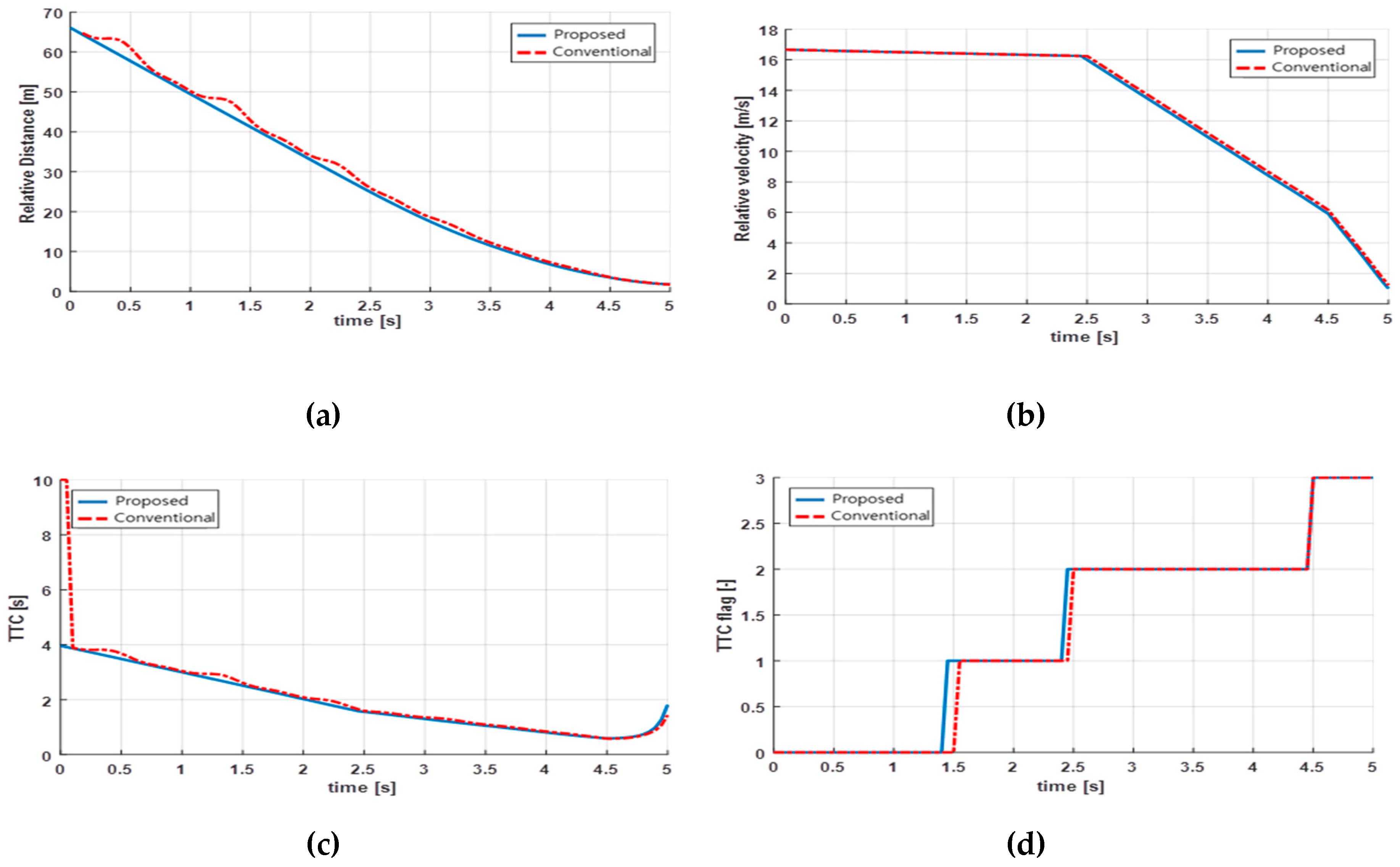
Figure 9 compares the performances of the AEB systems on a curve with constant curvature. As the conventional AEB system always assumed a constant curvature, it was expected that both the AEB systems would exhibit similar performances.
As the host vehicle initially moved at an even velocity and was slowed down by TTC, it initially exhibited a uniform motion, followed by a uniformly accelerated motion. Accordingly, the relative distance between the two vehicles decreased at a constant rate, and the gradient showed a gradual changed only during deceleration. In
Figure 9a, as previously expected, the conventional AEB system and the proposed AEB system exhibited a constant decrease in velocity, and the gradient had a gradual change when the TTC flag operated at partial and full braking. In addition, the proposed AEB system and conventional AEB system had similar relative distances, with initial relative distances of 64.3 m and 64.7 m, respectively, and ultimate relative distances of 1.8 m and 1.7 m, respectively. The relative velocities and times for TTC and TTC flag indicated that the AEB systems operated at similar points. Finally, comparing the results of the four parameters, both AEB systems yielded similar performances on a constant curvature.
The proposed AEB system and the conventional AEB system had initial relative distances of 99.9 m and 91.9 m, respectively, and ultimate relative distances of 1.12 m and 0.02 m, respectively. Since each vehicle had the same initial position, the initial relative distance needed to be similarly estimated. However, the difference between the initial relative distances of the two AEB systems is about 10 m.
The proposed AEB system on the curve road is the same as the AEB system on straight roads through the transformation of the curvature coordinate system. Therefore, in the proposed AEB system, the relative distance decreases slowly and constantly, whereas in the existing AEB system, there is a section in which the phase distance changes rapidly. This indicates that the proposed AEB system accurately derived the relative distance irrespective of the alignment of the curve road, and performed appropriate braking accordingly. On the other hand, when the relative distance increased sharply at the point where the road changed direction (4.8s), the relative distance affected the operating timing of the partial braking and full braking in the existing AEB system. Therefore, because the final relative distance is too close, the existing AEB system does not seem to be able to avoid the collision in Scenario 2.
5. Discussion
This study examined the improvement of the performance of a curvilinear coordinate-based AEB system. The proposed AEB system derived collision risks for each road environment by using the position and velocity information of the host and target vehicles, which were obtained through V2V communication. In addition, as the proposed AEB system calculated relative distances by converting the information of the host and target vehicles from an orthogonal coordinate to a curvilinear coordinate, the geometrical complexity of roads could be considered when determining the actuation time of the AEB system.
To verify the proposed AEB system, a simulation was conducted by linking MATLAB/Simulink and PreScan. Furthermore, the effectiveness of the proposed algorithm was analyzed by comparing the simulation results between the proposed AEB system and the conventional AEB system for a curve with constant curvature and a reversed curve.
The conventional and proposed AEB systems produced the following simulation results. Both AEB systems showed similar performance for a curve with constant curvature. However, for a reversed curve, the conventional AEB system, which did not reflect the geometric factors of the curve, could not accurately estimate the relative distance, a necessary parameter for deriving a collision risk. Accordingly, the conventional AEB system was delayed in actuating the braking, such that the final result was close to a collision. On the other hand, the proposed AEB system generated an average relative distance of 1 m. Thus, the proposed AEB system had a better performance than the conventional AEB system.
This study proposed a curvilinear coordinate-based AEB system that considered various curvatures. The results revealed that the proposed AEB system could be effective in various driving environments. Finally, since this system can be applicable to road environments other than curves, it will contribute to advancing AEB technology.


