Urban Air Quality Analysis and Forecast Based on Intelligent Algorithm with Parameter Optimization and Decision Rules

Featured Application

Air pollution has become an unavoidable reality in today’s world. With the rapid development of various industries and motorized transportation, large amounts of harmful substances such as soot, sulfur dioxides, nitrogen oxides, carbon monoxides, and hydrocarbons are released into the atmosphere, lasting a long time and in concentrations exceeding tolerable environmental limits. In this study, we investigated an intelligent algorithm that had the functions of parameter optimization and decision rules, which we applied to Beijing air quality data to analyze and forecast urban air quality.

Abstract

Air pollution has an ongoing devastating impact on the planet, damaging ecosystems, depleting natural resources, and endangering human health. This paper proposes a new intelligent algorithm that includes parameter optimization and decision rules to forecast and analyze of urban air quality. Through analysis of 24-h daily air quality data provided by the Beijing Air Quality Monitoring Station, simulated annealing (SA) and a decision tree (DT) emerge as the key factors. We prove that in the investigated algorithm, SA and DT can be used to make decision rules and achieve better accuracy for classification. We find that SA can be used to adjust the best parameter settings for the DT. Simulation results show that the accuracy of the proposed algorithm for classification is far better than other existing approaches.

1. Introduction

With the global trend and people’s attention, how to monitor the air quality scientifically and effectively and how to further prevent and control air pollution has become a hot topic. The problem of air pollution is very complex, which is characterized by multi pollution coexistence, multi-scale correlation, and multi process evolution. In order to solve this complex problem, it is particularly important to strengthen the construction of air quality monitoring and air quality management information. Only effective prediction, analysis, and research on air quality can effectively improve air quality. How to effectively use the real-time monitoring data of each city’s automatic air monitoring station, mine its internal information, use the monitoring data to build a bridge for analyzing the pollution problem [1], effective improvement of air quality, improvement of people’s living environment to maintain people’s health is an urgent problem to be solved.

The air quality index (AQI) is calculated by monitoring the concentration of fine particulate matter (PM_2.5), inhalable particulate matter (PM₁₀), sulfur dioxide (SO₂), nitrogen dioxide (NO₂₎, ozone (O₃), and carbon monoxide (CO). In recent years, due to the increasing consumption of various energy resources and the increase of cumulative emissions, the problem of air pollution has seriously increased. More and more attention has been paid to the study of air pollution. In order to better adapt to the global trend and create a good air environment, using data mining technology to establish air quality analysis, the forecast model has become an important topic [2,3,4,5,6,7,8,9].

Collecting AQI data is key for monitoring pollution problems. To solve the AQI problem, various approaches have been used for data mining, including artificial neural network (ANN), genetic algorithm (GA), decision tree (DT), random forest (RF), and support vector machine (SVM) [10,11,12,13,14,15,16,17,18,19,20]. Each method has a single basic point of view and provides a general performance analysis of air quality indicators, but it is difficult to distinguish the best method. Recent studies have proposed various intelligent systems, and the results seem applicable [21,22,23,24,25,26]. However, these investigated methods have an important shortcoming: they cannot simultaneously provide parameter optimization for an algorithm as well as decision rules. For AQI evaluation, decision rules can be updated according to datasets in the evaluation process and can be used to predict new evaluation results. For that we would aim to investigate an algorithm based on the characteristics of AQI decision rule establishment and parameter optimization. Then the urban air quality forecast and analysis can be based on an intelligent algorithm with parameter optimization and decision rules. We therefore propose an intelligent algorithm that combines DT and simulated annealing (SA), in which DT generates decision rules and SA converges to a global optimum, and the parameters of DT are determined by SA. The rules extracted in this paper could be used to analyze collected information, then forecast a new AQI. In what follows, we review the decision tree in Section 2, introduce the proposed algorithm in Section 3, and analyze the simulation results and discussions in Section 4. Finally, we draw the conclusion.

2. A Brief Description of the Decision Tree Algorithm

In our previous work [27,28], we applied the DT algorithm in anomaly intrusion detection and found it to have excellent classification performance. The DT has the advantages of intuitive expression and convenient operation and is widely used in research [29,30,31,32,33,34,35,36]. It consists of a root node, a child node, and a leaf node. After the structure is established, the required data are tested, starting from the root node. Depending on the different data attributes, the sub-node selects a property and moves to another sub-node recursively until the leaf is reached. Nodes and leaf nodes are the classifications for data prediction. When a DT is constructed, the attribute with the highest information gain rate is the split attribute of the current node. With recursive calculation, the information gain rate of the calculated attributes becomes smaller and smaller, and in the latest stage, the attribute with relatively large information gain rate will be selected as the splitting attribute, and the DT uses the Gini coefficient minimization criterion to perform feature selection to generate a binary tree [29,30]. The Gini coefficient minimization criterion is calculated as follows:

$$Gini\left(p\right)={\displaystyle \sum _{k=1}^k}{p}_k\left(1-p_k\right)=1-{\displaystyle \sum _{k=1}^k}{p}_k^2$$

(1)

$p_k$ indicates the probability that the selected sample belongs to the k class; the probability that the sample is split is $\left(1-p_k\right)$. For a given sample set $D$, the Gini index is:

$$Gini\left(D\right)=1-{\displaystyle \sum _{k=1}^k}{\frac{\left|{\complement }_k\right|}{\left|D\right|}}^2$$

(2)

Here, ${\complement }_k$ is the sample belonging to the $k^{th}$ class in $D$, and $k$ is the number of classes. If the sample set $D$ is divided into two parts $D_1$ and $D_2$ according to whether a feature A takes a certain value a, namely:

$$D_1=\left\{\left(\left(x,y\right)\in D|A\left(x\right)\right)=a\right\},D_2=D-D_1$$

(3)

then under the condition of feature $A$, the Gini index of set $D$ is defined as:

$$Gini\left(D,A\right)=\frac{\left|D_1\right|}{\left|D\right|}Gini\left(D_1\right)+\frac{\left|D_2\right|}{\left|D\right|}Gini\left(D_2\right)$$

(4)

The Gini index Gini $\left(D\right)$ represents the uncertainty value of the set $D$, and the Gini index Gini (D, A) represents the uncertainty value of the set $D$ after $A=a$ partitioning. The larger the Gini index value, the greater the uncertainty result of the sample set. When using the DT algorithm, the two parameters of minimum case ($M$) and the pruning confidence factor ($CF$) will have different combinations when facing different problems or cases [29]. In this paper, the SA algorithm is used to adjust and determine the best combination of these two parameters and the best solution of the problem.

3. The Proposed Algorithm

This paper proposes an algorithm for urban air quality forecast and analysis that is based on an intelligent algorithm with parameter optimization and decision rules. In the study, in order to verify the performance of the proposed algorithm, we use Beijing air quality data in CSV (Comma-Separated Values) format [37]. A partial original data is shown in

Table 1. Partial original data for the the Beijing dataset.

Date	Hour	Type	Dongcheng	Tiantan	Guanyuan	Yungang
20180101	0	Fine particulate matter (PM2.5)	77	60	65	52
20180101	0	PM2.5_24h
20180101	0	Inhalable particulate matter (PM10)	139	86	139	97
20180101	0	PM10_24h
20180101	0	Air quality index (AQI)	103	81	95	74
20180101	1	PM2.5	71	60	56	66
20180101	1	PM2.5_24h
20180101	1	PM10	125	98	109	121
20180101	1	PM10_24h
20180101	1	AQI	95	81	80	89
20180101	2	PM2.5	42	63	37	37
20180101	2	PM2.5_24h
20180101	2	PM10	78	93	73	77
20180101	2	PM10_24h
20180101	2	AQI	64	85	62	64
20180101	3	PM2.5	38	39	35	34
20180101	3	PM2.5_24h
20180101	3	PM10	67	61	72	63
20180101	3	PM10_24h
20180101	3	AQI	59	56	61	57
20180101	4	PM2.5	33	27	38	36
20180101	4	PM2.5_24h
20180101	4	PM10	65	50	78	67
20180101	4	PM10_24h

. The seven different features are listed in

Table 2. The seven features of air quality applied to the Beijing dataset.

PM2.5	Particles in the atmosphere with a diameter less than or equal to 2.5 μm, also known as particulate matter, have an important effect on air quality and human health.
PM10	Particulate matter in the atmosphere with a diameter of 10 μm or less is known as fly ash. This can enter the lungs, and it has an important impact on air quality and human health.
SO2	Sulfur dioxide is one of the main atmospheric pollutants. When sulfur dioxide is dissolved in water, sulfurous acid is formed, the main component of acid rain.
NO2	Nitrogen dioxide comes mainly from high-temperature combustion processes, such as vehicle exhaust and boiler exhaust emissions. It’s another cause of acid rain, which reduces atmospheric visibility and contributes to the acidification and eutrophication of surface water.
O3	The increasing concentration of ozone in the troposphere has a detrimental effect on human health and plants. Ozone has a stimulating effect on the eyes and respiratory organs and at above-normal levels negatively affects lung function.
CO	Carbon monoxide easily combines with hemoglobin to form carboxyhemoglobin, which prevents hemoglobin from carrying oxygen and causes tissue suffocation and death. Carbon monoxide has toxic effects on all body tissue cells, especially the cerebral cortex.
AQI	As the AQI increases, air quality worsens and pollution becomes more serious.

[38]. As shown in Table 2, these pollutants cause poor air quality, affect human living environment and harm human health. The real-time historical data of AQI from 1 January 2017 to 6 October 2018 in the District of Dongcheng, Beijing, 11270 AQI instances with seven different features were collected.

Table 3. Partial AQI data for the District of Dongcheng.

PM2.5	PM10	SO2	NO2	O3	CO	AQI
77	139	13	93	3	2	103
71	125	12	83	3	1.8	95
42	78	7	66	2	1.4	64
38	67	7	67	2	1.3	59
33	65	6	65	2	1.1	58
23	51	6	58	3	1	51
22	39	4	49	8	0.9	39
16	34	4	43	13	0.8	34
18	34	5	47	10	0.9	34
12	33	4	34	24	0.8	33
15	34	5	26	33	0.8	34
13	29	4	25	38	0.9	29
12	19	4	17	47	0.7	19
12	16	6	18	50	0.7	17
19	30	9	25	47	0.9	30
23	39	10	27	43	1	39
30	51	10	39	35	1.2	51
47	77	15	62	18	1.7	65
64	110	30	83	3	2.8	86
72	138	40	81	2	3.1	96
66	142	39	73	4	2.7	96
67	126	23	61	8	2	90
67	126	18	64	5	1.8	90
38	70	8	40	20	1	60

presents partial data for the resulting AQI.

According to Environmental Air Quality Standards GB 3095-2012, discrete AQI data are classified according to pollution levels one (excellent) through six (serious). The corresponding relationship between AQI and air quality level is shown in

Table 4. Relationship between AQI and air quality level.

No.	AQI	Air Quality Level
1	0–50	Level 1: Excellent
2	51~100	Level 2: Good
3	101~50	Level 3: Light pollution
4	151~200	Level 4: Medium pollution
5	201~250	Level 5: Heavy pollution
6	251~300	Level 6: Serious pollution

.

Table 5. Partial data for air quality level.

PM2.5	PM10	SO2	NO2	O3	CO	Level
77	139	13	93	3	2	3
71	125	12	83	3	1.8	2
42	78	7	66	2	1.4	2
38	67	7	67	2	1.3	2
33	65	6	65	2	1.1	2
23	51	6	58	3	1	2
22	39	4	49	8	0.9	1
16	34	4	43	13	0.8	1
18	34	5	47	10	0.9	1
12	33	4	34	24	0.8	1
15	34	5	26	33	0.8	1
13	29	4	25	38	0.9	1
12	19	4	17	47	0.7	1
12	16	6	18	50	0.7	1
19	30	9	25	47	0.9	1
23	39	10	27	43	1	1
30	51	10	39	35	1.2	2
47	77	15	62	18	1.7	2
64	110	30	83	3	2.8	2
72	138	40	81	2	3.1	2
66	142	39	73	4	2.7	2
67	126	23	61	8	2	2
67	126	18	64	5	1.8	2
38	70	8	40	20	1	2

presents partial data for air quality level.

Metropolis introduced SA and proposed an importance sampling method—i.e., accepting new states with probability—called the Metropolis criterion [39]. This is the basic idea of SA algorithms. Kirkpatrick et al. first proposed the simulated annealing algorithms in 1983 [40,41]. SA makes the optimal solution asymptotically convergent and is widely used to solve optimization problems. In recent years, with the rapid increase of information, there has been a huge amount of data (big data) which is larger than the traditional data. Under such a large amount of AQI data, how to find useful data from it has become an important issue. DT is based on the tree structure, presenting the data rules, enabling analysts to understand the implicit knowledge of the data and interpret it, which is widely used in various fields [30,31,32]. However, before establishing the decision tree model, it is necessary to set its relevant parameters, which will affect the result. Under different parameter combinations, if the parameter values are not adjusted properly, the classification result will be poor. Because parameters minimum case (M) and the pruning confidence factor ($CF$) of the DT will be different due to different problems, it is very time-consuming to manually adjust them.

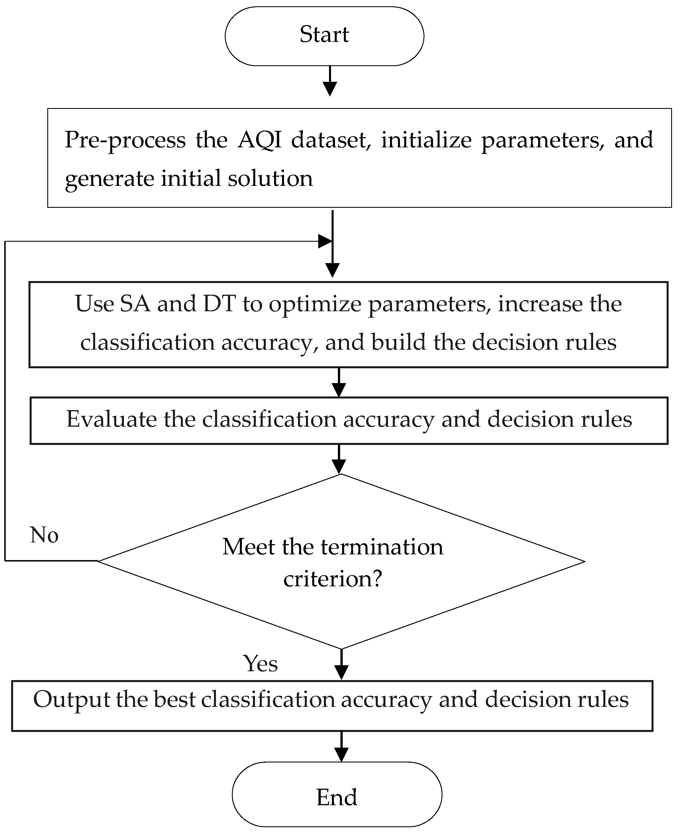
Therefore, this paper proposes an intelligent algorithm combining DT and SA, and studies an algorithm based on AQI decision rule establishment and parameter optimization. Then, based on the intelligent algorithm of parameter optimization and decision rules, the urban air quality is predicted and analyzed. This study combines the advantages of DT and SA. DT generates decision rules, SA converges to the global optimum, and the parameters minimum case (M) and the pruning confidence factor ($CF$) of the DT determined by SA. The rules extracted in this paper can be used to analyze the collected information and then forecast a new AQI.

Figure 1 shows a flow chart of the proposed algorithm; the AQI dataset is pre-processed as training and testing data, then initial values for the parameters are proposed; after that, the initial solution can be generated randomly. The proposed algorithm begins with four parameters, namely $I_{gen},T_0,T_f,\mathrm{and}\lambda$, where $I_{gen}$ denotes the number of generations, $T_0$ represents the initial temperature, $T_f$ represents the final temperature that stops the proposed algorithm if the current temperature is lower than $T_f$, and $\lambda$ is the coefficient controlling the cooling rate,, respectively. The current temperature $T$ is set to be the same as $T_0$. The solution is represented as seven features followed with two variables $M$, and $CF$ as shown in

Table 6. A representation of the solution.

Feature#1

Feature#2

Feature#3

Feature#4

Feature#5

Feature#6

Feature#7

M

CF

. An initial solution $\mathsf{\alpha }$ is randomly generated according to the representation of solution in Table 6. For each generation, the next solution $\beta$ is generated from $\mathsf{\alpha }$ by randomly swapping these seven features and randomly generating these values of four variables in the current solution. T is decreased after running $I_{gen}$ generations, according to a formula $T\leftarrow \lambda T$, where 0 < $\lambda$ < 1. Let $obj\left(\alpha \right)$ denotes the testing accuracy of $\mathsf{\alpha }$, and $\Delta$ denote the difference between $obj\left(\alpha \right)$ and $obj\left(\beta \right)$; that is $\Delta =obj\left(\alpha \right)-obj\left(\beta \right)$. The probability of replacing $\alpha$ with $\beta$, where $\alpha$ is the current solution and $\beta$ is the next solution, given that $\Delta$ > 0, is $e^{-\Delta /T}$. This is accomplished by generating a random number $r$ ∈ [0,1] and replacing the solution with $\beta$ if <$e^{-\Delta /T}$. Meanwhile, if $\Delta$ ≤ 0, the probability of replacing $\alpha$ with $\beta$ is one. In the proposed algorithm, SA and DT are performed to optimize parameters ($M$ and $CF$) to increase the testing accuracy for selected features and build the decision rules. The proposed algorithm is repeated until $T$ is lower than $T_f$. Thereafter, the best testing accuracy, and decision rules are reported.

The proposed approach uses the accuracy based on the confusion matrix, which can test the performance of the classification method. The confusion matrix is shown as

Table 7. The confusion matrix.

Actual Predicted	Actual Positive	Active Negative
Predicted Positive	TP (True Positive)	FP (False Positive)
Predicted Negative	FN (False Negative)	TN (True Negative)

.

TP, FP, FN, and TN represent true positive class, false positive class, false negative class, and true negative class, respectively. The predicted value is a positive example, which is recorded as P (positive). The predicted value is a negative example, which is recorded as N (negative). When the predicted value is the same as or opposite to the actual value, they are recorded as T (true) or F (false), respectively. Four results of defining of examples in the dataset after model classification are: TP: predicted positive class or actually positive class; FP: predicted positive class or actually negative class; TN: predicted negative class or actually negative class; FN: predicted negative class or actually positive class. The classification accuracy calculation formula is as follows:

Classification accuracy = (TP + TN)/(TP + FN + FP + TN) × 100%

(5)

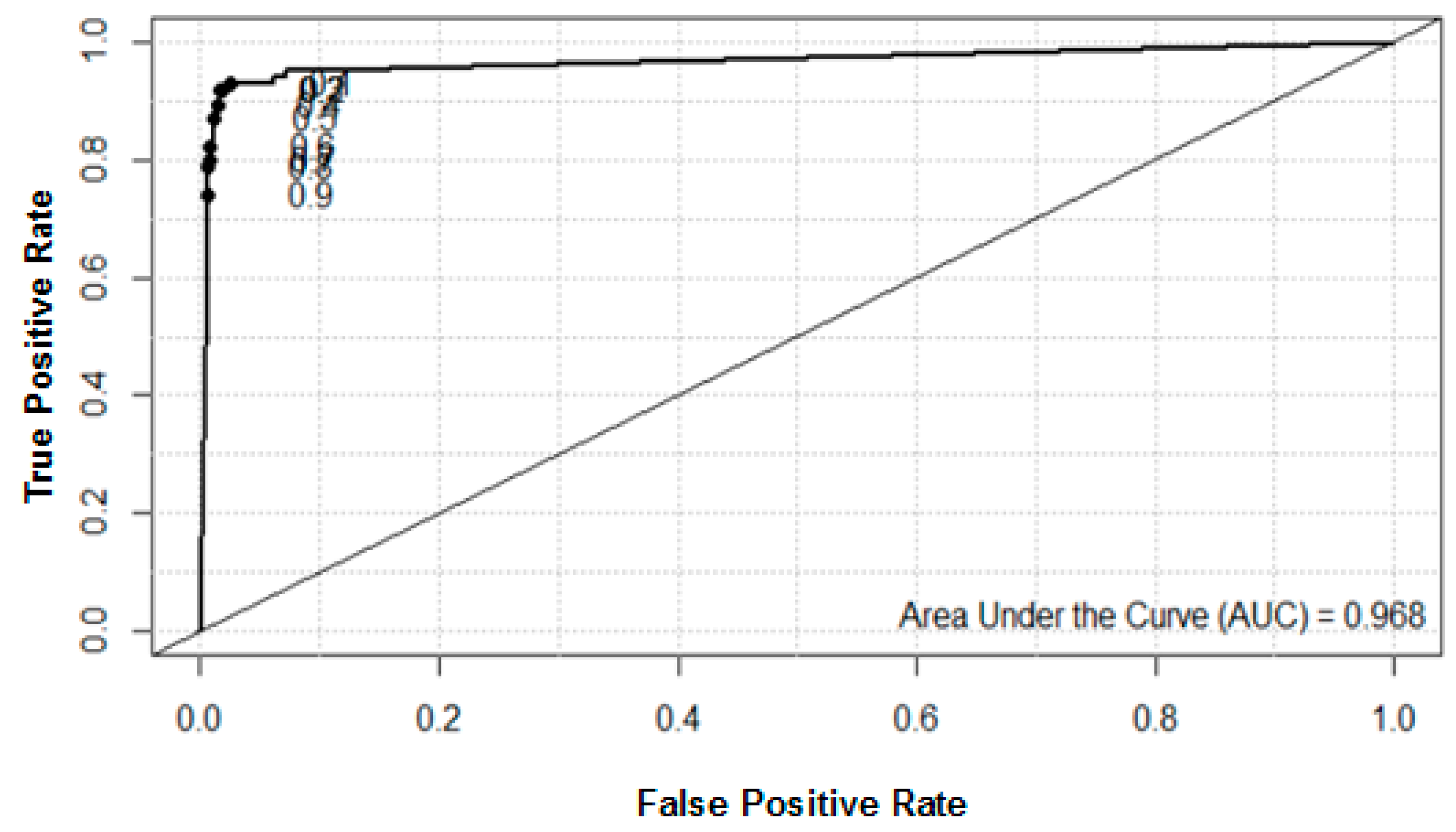
The receiver operating characteristic curve (ROC curve) and area under the curve (AUC) can test the performance of classification results. Because ROC curve has a good characteristic, when the distribution of positive and negative samples in the test set is changed, ROC curve can be still unchanged. Class imbalance often occurs in the actual data set, that is, there are many more negative samples than positive samples (or vice versa), and the distribution of positive and negative samples in the test data may change with time. The area under ROC curve is calculated as the evaluation method of imbalanced data. It can comprehensively describe the performance of classifier under different decision thresholds. AUC calculation formula is as follows:

$$\mathrm{AUC}=\frac{1+\left(\frac{\mathrm{TP}}{\mathrm{FP}+\mathrm{FN}}\right)-\left(\frac{\mathrm{FP}}{\mathrm{TN}+\mathrm{FP}}\right)}{2}$$

(6)

4. Simulation Results and Discussions

This study adopts 10-fold cross-validation to evaluate results. The data was divided into 10 portions. Nine portions of data were retrieved as training data and the other one was used for testing data. To verify its performance, the proposed algorithm was used with the RF and SVM approaches, and the simulation results were compared. The SVM is a learning system that uses a hypothesis space of linear function in a high-dimensional feature space. The RF is an ensemble learning method for classification that constructs multiple decision trees at training time, and outputs the class that depends on the majority of the classes. The SA parameters were set to the number of generations $I_{gen}$ = 5000, the initial temperature $T_0$ = 100, the final temperature $T_f$ = 0.01, and the cooling rate λ = 0.95 [42]. The search range of the DT parameter named $M$ was changed from 2 to 100 and that of $CF$ was changed from 0.01 to 0.5.

4.1. Comparative Analysis of Classification Accuracy with Proposed Algorithm and Other Methods

The simulation results in

Table 8. Comparison of classification accuracy using different approaches.

	Decision Tree (DT)	Random Forest (RF)	Support Vector Machine (SVM)	The Proposed Algorithm
Classification accuracy	95.34	98.81	99.14%	99.92%

show the classification accuracy of the proposed algorithm and other approaches using training data. From Table 8, it can be found that the proposed algorithm has a classification accuracy of 99.92%, which is better than other approaches such as decision tree (DT), random forest (RF), and support vector machine (SVM). As can be seen from Table 8, the classification accuracy of the only DT is 95.34%, and the classification accuracy of the proposed algorithm is 99.92%, which means that the SA algorithm has an additive effect on DT, and the parameters can be adjusted to improve its accuracy. Because SA has the advantage of jumping out of local optimum according to probability, it can effectively prevent the search process from falling into a local optimum. This paper proposes an intelligent algorithm SA added to DT. Using the advantages of SA, the $M$ and $CF$ in DT can be effectively determined.

4.2. Analysis of Decision Rules Obtained from the Proposed Algorithm

The obtained decision rules have a total of eight DT rules, which are shown in

Table 9. Decision rules obtained from the proposed algorithm.

No.	Rules
1	When PM2.5 < 49.5 and PM10 < 35.5, the air quality rating is 1. It means, data required to start the test from the root node PM2.5 < 49.5. According to different data attributes, it moves to the sub node PM10 < 35.5, finally reaches the leaf node of the air quality level 1.
2	When PM2.5 < 49.5 and PM10 ≥ 35.5, the air quality rating is 2. It means, data required to start the test from the root node PM2.5 < 49.5. According to different data attributes, it moves to the sub node PM10 ≥ 35.5, finally reaches the leaf node of the air quality level 2.
3	When PM2.5 ≥ 49.5, PM10 < 74.5 and PM2.5 < 150.5, the air quality rating is 2. It means, data required to start the test from the root node PM2.5 ≥ 49.5. According to different data attributes, it moves to the sub node PM10 < 74.5, then recursively moves to another sub node PM2.5 < 150.5, finally reaches the leaf node of the air quality level 2.
4	When PM2.5 ≥ 49.5, PM10 < 74.5 and PM10 ≥ 150.5, the air quality rating is 3. It means, data required to start the test from the root node PM2.5 ≥ 49.5. According to different data attributes, it moves to the sub node PM10 < 74.5, then recursively moves to another sub node PM2.5 ≥ 150.5, finally reaches the leaf node of the air quality level 3.
5	When PM2.5 ≥ 49.5, PM10 ≥ 74.5 and PM10 < 114.5, the air quality evaluation level is 3. It means, data required to start the test from the root node PM2.5 ≥ 49.5. According to different data attributes, it moves to the sub node PM10 ≥ 74.5, then recursively moves to another sub node PM10 < 114.5, finally reaches the leaf node of the air quality level 3.
6	When PM2.5 ≥ 49.5, PM10 ≥ 74.5 and PM10 ≥ 114.5, further judging that when PM10 < 149.5, the air quality evaluation level is 4. It means, data required to start the test from the root node PM2.5 ≥ 49.5. According to different data attributes, it moves to the sub node PM10 ≥ 74.5, then recursively moves to another sub node PM10 ≥ 114.5, then recursively moves to another sub node PM10 < 149.5, finally reaches the leaf node of the air quality level 4.
7	When PM2.5 ≥ 49.5, PM10 ≥ 74.5 and PM10 ≥ 114.5, it is further judged that when PM10 ≥ 149.5 and PM10 < 249.5, the air quality rating is 5. It means, data required to start the test from the root node PM2.5 ≥ 49.5. According to different data attributes, it moves to the sub node PM10 ≥ 74.5, then recursively moves to another sub node PM10 ≥ 114.5, then recursively moves to another sub node PM10 ≥ 149.5, then recursively moves to another sub node PM10 < 249.5, finally reaches the leaf node of the air quality 5.
8	When PM2.5 ≥ 49.5, PM10 ≥ 74.5 and PM10 ≥ 114.5, it is further judged that when PM10 ≥ 149.5 and PM10 ≥ 249.5, the air quality rating is 6. It means, data required to start the test from the root node PM2.5 ≥ 49.5. According to different data attributes, it moves to the sub node PM10 ≥ 74.5, then recursively moves to another sub node PM10 ≥ 114.5, then recursively moves to another sub node PM10 ≥ 149.5, then recursively moves to another sub node PM10 ≥ 249.5, finally reaches the leaf node of the air quality 6.

. PM_2.5 and PM₁₀ are the main factors that will affect air quality. The DT is divided by PM_2.5 as the root node, indicating that PM_2.5 is the most important indicator that will affect air quality level.

4.3. Analysis of Factors Influencing Air Quality

To illustrate the extent of the air quality influence factor,

Table 10. Increased node purity (IncNodePurity) values for the air quality influence factor.

Influence Factor	IncNodePurity
PM2.5	3041.97839
PM10	2734.23447
SO2	193.65775
NO2	142.87993
O3	60.44758
CO	159.37930

presents the results of using the values of influence factors from IncNodePurity (increased node purity) for air quality. IncNodePurity is an evaluation method that can use the non-negative sum of residuals to find a simulated value. This value can elucidate the extent to which the various important factors affect air quality. An influence factors diagram is shown in Figure 2. Table 10 and Figure 2 indicate the influence factors to be PM_2.5 > PM₁₀ > SO₂ > CO > NO₂ > O₃. It can also be seen that the value of the IncNodePurity of PM_2.5 is the largest, which suggests that PM_2.5 has the greatest impact on air quality.

4.4. Air Quality Data Set Analysis of ROC and AUC

In our implementation, the area under the receiver operating characteristic (ROC) curve is the area under the curve (AUC), which is used to evaluate the performance of the proposed approach. The value of AUC varies from 0 to 1, with larger values being better. In Figure 3, the value of AUC for the air quality data set is 0.968, demonstrating that the proposed algorithm performs well.

5. Conclusions

This paper has proposed urban air quality analysis and a forecast based on an intelligent algorithm with parameter optimization and decision rules. The proposed algorithm was applied to test the AQI using Beijing’s dataset. SA and DT were used to achieve the best classification accuracy and classify air quality by the obtained decision rules, and they were shown to be efficient for generating decision rules. In addition, parameters minimum case ($M$) and the pruning confidence factor ($CF$) of the DT were calculated and applied automatically. This research provided a prediction model for improving air quality and this model could effectively improve people’s living environment protect people’s health. In our implementation, the training data accuracy classification was 99.92%, the air quality impact factors were sorted as PM_2.5 > PM₁₀ > SO₂ > CO > NO₂ > O₃, and the AUC value for the air quality data set was 0.968. From the simulation results, we determined that the performance of the proposed algorithm is better than that of other current approaches.

Further research will focus on the following aspects: (1) using a simulated annealing algorithm for other data mining technologies (such as support vector machines, neural networks, etc.) to find the best parameters and improve the accuracy of the method; (2) improving the algorithm or combining the advantages of other algorithms to conduct data mining and compare the results.

References

1. Wang, Y.C.; Chen, G.W. Efficient Data Gathering and Estimation for Metropolitan Air Quality Monitoring by Using Vehicular Sensor Networks. IEEE Trans. Veh. Technol. 2017, 66, 7234–7248. [Google Scholar] [CrossRef]
2. Yang, Y.Z.; Zheng, Z.J.; Bian, K.G.; Song, L.Y.; Han, Z. Real-Time Profiling of Fine-Grained Air Quality Index Distribution Using UAV Sensing. IEEE Internet Things J. 2018, 5, 186–198. [Google Scholar] [CrossRef]
3. Mei, S.K.; Li, H.; Fan, J.; Zhu, X.J.; Dyer, C.R. Inferring air pollution by sniffing social media. In Proceedings of the 2014 IEEE/ACM International Conference on Advances in Social Networks Analysis and Mining, Beijing, China, 17–20 August 2014; pp. 534–539. [Google Scholar]
4. Margan, B.; Hakimpour, F.; Saber, M. Linked data geo-statistical analysis of air pollution in urban areas. In Proceedings of the 2018 4th International Conference on Web Research (ICWR), Tehran, Iran, 25–26 April 2018; pp. 86–91. [Google Scholar]
5. Wang, L.P.; Chen, J. Socio-economic influential factors of haze Pollution in China: Empirical study by eba model using spatial panel data. Acta Sci. Circumstantiae 2016, 36, 3833–3839. [Google Scholar]
6. Qin, Y.C.; Xie, Z.X.; Li, Y. Review of research on the impacts of atmospheric pollution on the health of residents. Environ. Sci. 2019, 40, 1512–1520. [Google Scholar]
7. Liu, W.Q.; Chen, Z.Y.; Liu, J.G. Atmospheric stereoscopic monitoring technology and development trend in China. Environ. Monit. China 2018, 34, 1–9. [Google Scholar]
8. Liu, W.Q.; Liu, J.G.; Xie, P.H. Spatio-temporal monitoring system and its application in regional complex air pollution study. J. Atmos. Environ. Opt. 2009, 4, 243–255. [Google Scholar]
9. Marcazzan, G.M.; Vaccaro, S.; Valli, G. Characterisation of PM10 and PM2.5 particulate matter in the ambient air of Milan (Italy). Atmos. Environ. 2001, 35, 4639–4650. [Google Scholar] [CrossRef]
10. Aggarwal, A.; Choudhary, T.; Kumar, P. A fuzzy interface system for determining Air Quality Index. In Proceedings of the 2017 International Conference on Infocom Technologies and Unmanned Systems, Dubai, UAE, 18–20 December 2017; pp. 786–790. [Google Scholar]
11. Kamalm, M.M.; Jailani, R.; Shauri, R.L.A. Prediction of Ambient Air Quality Based on Neural Network Technique. In Proceedings of the 2006 4th Student Conference on Research and Development, Selangor, Malaysia, 27–28 June 2006; pp. 115–119. [Google Scholar]
12. Xue, H.X.; Bai, Y.P.; Hu, H.; Xu, T.; Liang, H. A Novel Hybrid Model Based on TVIW-PSO-GSA Algorithm and Support Vector Machine for Classification Problems. IEEE Access 2019, 7, 27789–27801. [Google Scholar] [CrossRef]
13. Mu, B.; Li, S.; Yuan, S.J. An improved effective approach for urban air quality forecast. In Proceedings of the 2017 13th International Conference on Natural Computation, Fuzzy Systems and Knowledge Discovery (ICNC-FSKD), Guilin, China, 29–31 July 2017. [Google Scholar]
14. Wang, W.; Shen, W.G.; Chen, B.; Zhu, R.; Sun, Y.X. Air Quality Index Forecasting Based on SVM and Moments. In Proceedings of the 2018 5th International Conference on Systems and Informatics (ICSAI), Nanjing, China, 10–12 November 2018; pp. 851–855. [Google Scholar]
15. Dai, H. Research on SVM improved algorithm for large data classification. In Proceedings of the IEEE 3rd International Conference on Big Data Analysis (ICBDA), Shanghai, China, 9–12 March 2018; pp. 181–185. [Google Scholar]
16. Vardoulakis, S.; Fisher, B.; Pericleous, K. Modelling air quality in street canyons: A review. Atmos. Environ. 2003, 37, 155–182. [Google Scholar] [CrossRef] [Green Version]
17. Lu, J.N.; Hu, H.P.; Bai, Y.P. Radial Basis Function Neural Network Based on an Improved Exponential Decreasing Inertia Weight-Particle Swarm Optimization Algorithm for AQI Prediction. Abstr. Appl. Anal. 2014. [Google Scholar] [CrossRef] [Green Version]
18. Teologo, A.T.; Dadios, E.P.; Baldovino, R.G.; Neyra, R.Q.; Javel, I.M. Air Quality Index (AQI) Classification using CO and NO2 Pollutants: A Fuzzy-based Approach. In Proceedings of the TENCON 2018—2018 IEEE Region 10 Conference, Jeju, Korea, 28–31 October 2018. [Google Scholar]
19. Shawabkeh, A.; Al-Beqain, F.; Redan, A.; SalemBenzene, M. Air Pollution Monitoring Model using ANN and SVM. In Proceedings of the 2018 Fifth HCT Information Technology Trends (ITT), Dubai, UAE, 28–29 November 2018. [Google Scholar]
20. Altinçöp, H.; Oktay, A.B. Air Pollution Forecasting with Random Forest Time Series Analysis. In Proceedings of the 2018 International Conference on Artificial Intelligence and Data Processing (IDAP), Malatya, Turkey, 28–29 September 2018. [Google Scholar]
21. Gore, R.W.; Deshpande, D.S. An approach for classification of health risks based on air quality levels. In Proceedings of the 2017 1st International Conference on Intelligent Systems and Information Management (ICISIM), Aurangabad, India, 5–6 October 2017; pp. 58–61. [Google Scholar]
22. Feng, J.B. Atmosphere Quality Monitoring and Analysis Based on Intelligent Algorithm. In Proceedings of the 2016 International Conference on Intelligent Transportation, Big Data & Smart City (ICITBS), Changsha, China, 17–18 December 2016. [Google Scholar]
23. Liu, S.R.; Cao, X.Q. Application of Intelligent Information Processing Technology for Air Quality Assessment. In Proceedings of the 2008 Fifth International Conference on Fuzzy Systems and Knowledge Discovery, Jinan, China, 18–20 October 2008. [Google Scholar]
24. Cao, L.T. Environment Air Quality Evaluation System Based on Genetic Arithmetic and BP Neural Network. In Proceedings of the 2008 International Conference on Intelligent Computation Technology and Automation (ICICTA), Changsha, China, 20–22 October 2008. [Google Scholar]
25. Shaban, K.B.; Kadri, A.; Rezk, E. Urban Air Pollution Monitoring System with Forecasting Models. IEEE Sens. J. 2016, 16, 2598–2606. [Google Scholar] [CrossRef]
26. Jiao, Y.; Wang, Z.F.; Zhang, Y. Prediction of Air Quality Index Based on LSTM. In Proceedings of the 2019 IEEE 8th Joint International Information Technology and Artificial Intelligence Conference (ITAIC), Chongqing, China, 24–26 May 2019. [Google Scholar]
27. Lin, S.W.; Ying, K.C.; Lee, C.Y.; Lee, Z.J. An intelligent algorithm with feature selection and decision rules applied to anomaly intrusion detection. Appl. Soft Comput. 2012, 12, 3285–3290. [Google Scholar] [CrossRef]
28. Lee, C.Y.; Lee, Z.J.; Peng, B.Y.; Lin, C.C.; Huang, H. Apply data mining to analyze the rainfall of landslide. MATEC Web Conf. 2017, 169, 01034. [Google Scholar] [CrossRef]
29. Quinlan, J.R. Induction of decision trees. Mach. Learn. 1986, 1, 81–106. [Google Scholar] [CrossRef] [Green Version]
30. Han, S.H.; Lu, S.X. A prediction model for telecom customer lifecycle based-on CART tree. In Proceedings of the 2010 7th International Conference on Service Systems and Service Management, Tokyo, Japan, 28–30 June 2010; pp. 1–4. [Google Scholar]
31. Li, M.A. Application of CART decision tree combined with PCA algorithm in intrusion detection. In Proceedings of the 2017 8th IEEE International Conference on Software Engineering and Service Science (ICSESS), Beijing, China, 24–26 November 2017; pp. 38–41. [Google Scholar]
32. Qi, Y.; Luo, B.F.; Wang, X.D.; Wu, L. Load pattern recognition method based on fuzzy clustering and decision tree. In Proceedings of the 2017 IEEE Conference on Energy Internet and Energy System Integration (EI2), Beijing, China, 26–28 November 2017; pp. 1–5. [Google Scholar]
33. Sabariah, M.T.M.K.; Hanifa, S.T.A.; Sa’adah, M.T.S. Early detection of type II Diabetes Mellitus with random forest and classification and regression tree (CART). In Proceedings of the 2014 International Conference of Advanced Informatics: Concept, Theory and Application (ICAICTA), Bandung, Indonesia, 20–21 August 2014; pp. 238–242. [Google Scholar]
34. Li, Y.H.; Guo, Z.Q.; Yang, J.; Fang, H.; Hu, Y.W. Prediction of ship collision risk based on CART. IET Intell. Transp. Syst. 2018, 12, 1345–1350. [Google Scholar] [CrossRef]
35. Bittencourt, H.R.; Clarke, R.T. Use of classification and regression trees (CART) to classify remotely-sensed digital images. In Proceedings of the 2003 IEEE International Geoscience and Remote Sensing Symposium. Proceedings (IEEE Cat. No.03CH37477), Toulouse, France, 21–25 July 2003; pp. 3751–3753. [Google Scholar]
36. Unkel, S.; Farrington, C.P.; Garthwaitep, H. Statistical methods for the prospective detection of infectious disease outbreaks: A review. J. R. Stat. Soc. Ser. A Stat. Soc. 2012, 175, 49–82. [Google Scholar] [CrossRef] [Green Version]
37. Chinese Meteorological Historical Data. Available online: http://beijingair.sinaapp.com/ (accessed on 31 January 2019).
38. Boulter, P.G.; Borken-Kleefeld, J.; Ntziachristos, L.; Vianna, M. Urban Air Quality in Europe. In Handbook of Environmental Chemistry; Springer: Berlin/Heidelberg, Germany, 2013; Volume 26, pp. 31–54. [Google Scholar]
39. Metropolis, N.; Rosenblush, A.W.; Rosenblush, M.N. Equation of state calculations by fast computing machines. J. Chem. Phys. 1953, 56, 1087–1092. [Google Scholar] [CrossRef] [Green Version]
40. Kirkpatrick, S.; Gelatt, C.D.; Vecchi, J.M.P. Optimization by simulated annealing. Science 1983, 220, 671–680. [Google Scholar] [CrossRef] [PubMed]
41. Osman, I.H. Metastrategy simulated annealing and tabu search algorithms for the vehicle routing problems. Ann. Oper. Res. 1993, 42, 421–451. [Google Scholar] [CrossRef]
42. Lin, S.W.; Lee, Z.J.; Ying, K.C.; Lee, C.Y. Applying hybrid meta-heuristics for capacitated vehicle routing problem. Expert Syst. Appl. 2009, 36, 1505–1512. [Google Scholar] [CrossRef]
Figure 1. A flow chart of the proposed algorithm.
Applsci 09 05445 g001
Figure 2. Air quality influence factor.
Applsci 09 05445 g002
Figure 3. Receiver operating characteristic (ROC) and area under the curve (AUC) for the AQI dataset.
Applsci 09 05445 g003