Prediction Interval Adjustment for Load-Forecasting using Machine Learning

Featured Application

Prediction interval adjustment designed to be used in the Real-Time Electricity Market in Mexico.

Abstract

Electricity load-forecasting is an essential tool for effective power grid operation and energy markets. However, the lack of accuracy on the estimation of the electricity demand may cause an excessive or insufficient supply which can produce instabilities in the power grid or cause load cuts. Hence, probabilistic load-forecasting methods have become more relevant since these allow an understanding of not only load-point forecasts but also the uncertainty associated with it. In this paper, we develop a probabilistic load-forecasting method based on Association Rules and Artificial Neural Networks for Short-Term Load Forecasting (2 h ahead). First, neural networks are used to estimate point-load forecasts and the variance between these and observations. Then, using the latter, a simple prediction interval is calculated. Next, association rules are employed to adjust the prediction intervals by exploiting the confidence and support of the association rules. The main idea is to increase certainty regarding predictions, thus reducing prediction interval width in accordance to the rules found. Results show that the presented methodology provides a closer prediction interval without sacrificing accuracy. Prediction interval quality and effectiveness is measured using Prediction Interval Coverage Probability (PICP) and the Dawid–Sebastiani Score (DSS). PICP and DSS per horizon shows that the Adjusted and Normal prediction intervals are similar. Also, probabilistic and point-forecast Means Absolute Error (MAE) and Root Mean Squared Error (RMSE) metrics are used. Probabilistic MAE indicates that Adjusted prediction intervals fail by less than 2.5 MW along the horizons, which is not significant if we compare it to the 1.3 MW of the Normal prediction interval failure. Also, probabilistic RMSE shows that the probabilistic error tends to be larger than MAE along the horizons, but the maximum difference between Adjusted and Normal probabilistic RMSE is less than 6 MW, which is also not significant.

1. Introduction

Load-forecasting is an important tool for decision-makers that helps them in the creation of policies for planning and operation of the power system [1]. Most of these decisions must be taken based on electric demand forecasts, and the lack of accuracy in the estimations will lead to an inefficient decision-making process [2].

Specifically, the lack of accuracy may cause overestimation or underestimation of electricity demand [3]. The former causes an excessive amount of electricity to be purchased and supplied to the system, which causes power balance disturbances and instabilities in the power grid. The latter, on the other hand, leads to a risky operation of the power system by restraining the production of electricity, which may lead to load cuts directly affecting electricity users.

In particular, short-term demand forecasting is highly difficult due to its requirement of quick response, the amount of information required, as well as its complexity. These models must take into consideration not only the electric consumption pattern of the region but also its regulatory requirements. For instance, the Mexican Electric Market (MEM) establishes that every short-term load forecast method must be capable of estimating 8 periods of 15 min ahead (2 h) [4].

Intending to improve the accuracy of load demand forecast, researchers have developed forecast methods for short-term, mid-term and long-term [5]. Mid-term and long-term load demand forecasting is closely related to planning activities (e.g., power system maintenance tasks and capacity expansion planning), whereas short-term forecasts are employed for the ongoing operation (e.g., everyday unit commitment).

The main characteristic of electricity demand is that it is mostly (if not completely) influenced by human behavior patterns [6]. In this regard, human behavior follows a certain tendency with cycling patterns. This is, we humans do mostly the same things (e.g., the time to wake, the time to go to sleep, job schedule, etc.) on a day-to-day basis around the same time (e.g., wake up early in the morning). For instance, most productive human adults work on a working week basis. Hence, a weekday electricity consumption pattern is not only different from weekend patterns, but also different from holidays patterns (which may fall within the working week). This means that every period of time has different needs in terms of electricity demand forecasting and those needs are also different for each type of day.

Regarding a more technical aspect, electricity load-forecasting can be performed by using only historical measurements or forecast predictors (i.e., future period loads). For instance, load forecasting can be done 1 h ahead in 15 min interval using only load data from the past hour, or to use the predicted 15 min load within the 1 h ahead horizon. In particular, it has been stated that the incorporation of recursive forecast predictors leads to better performance in time series prediction [7]. Furthermore, if for each forecast horizon (i.e., 15 min ahead) a different model is trained, performance deterioration related to more distant forecasting horizons can be avoided (for instance, by using individual forecasting models for every 15 min) [7].

Therefore, an effective load-forecasting model must consider such patterns. In this paper, we investigate a modeling approach based on association rules (association rules are useful to describe a model in terms of cause and effect). The proposed approach aims at predicting electricity demand for two hours ahead in 8 periods of 15 min. The dataset is from a representative load zone of Mexico, which is 15-min load demand measures. The prediction intervals are estimated using Artificial Neural Network models. Then, the prediction intervals are adjusted through association-rule mining algorithms.

2. Literature Review

Unlike other Data Mining (DM) algorithms such as artificial neural network (ANN) or Random Forest (RF), association rules are not so popular regarding time series prediction. One reason is that these types of algorithms are usually associated with the design of expert systems which have fallen into disuse. For instance, in a recent review of DM algorithms applied to electricity time series forecasting [8], from the more than 100 works reviewed only 6 corresponded to algorithms using rule-based prediction. Nevertheless, regarding time series prediction, in [9] they proposed to use an ensemble of forecasting algorithm which is combined using fuzzy rule-based forecasting. The purpose of the latter is to determine the best weights for each forecasting method, such that the dependence between forecasting methods and time series statistical properties is aligned. The fuzzy rules are selected using linguistic association mining given the statistical properties of the time series. Using classical time series point forecasting methods, the proposed ensemble algorithm is tested against individual and the equal-weights ensemble employing the M3 competition time series. They found that the proposed ensemble performs slightly better than the tested algorithms.

In a more recent work [10], a modified a priori-based association-rule mining algorithm based on the Continuous Target Sequential Pattern Discovery (CTSPD) is proposed, it is then used to generate a set of association rules that help in predicting the concentration of air pollutants in New Delhi. In this work, time-dependent features from air pollutants time series are identified first to conform new variables (i.e., frequent sequences), which are then used (in the form of association rules) to predict the concentration of air pollutants. Their results showed that the proposed approach performed better than the India System of Air Quality and Weather Forecasting and Research (SAFAR). Similarly, in [11] authors propose an improved a priori algorithm for temporal data mining of frequent item sets in time series. This improved algorithm is focused on reducing the computational burden of identifying all frequent item sets, by constraining temporal relations. In this sense, this algorithm determines time constraints intervals, which are then used to filter (using the time interval algebra) and mine the corresponding transactions from the database. The method is compared against the classical a priori algorithm, obtaining a better performance regarding the storage and time required to mine rules.

On the other hand, an approach to the analysis of the electricity demand required by home appliances is proposed in [12]. In such work, several unsupervised learning algorithms (among them association rules) are employed in the identification of appliances energy consumption patterns. Using sequential rules, authors found that there exists a heavy interdependence between the usage patterns of home appliances, the time of the use, and the user activities. In the same fashion, a more recent work related to the analysis of smart metering analysis using a Big Data infrastructure is presented in [13]. By employing unsupervised data clustering and frequent pattern mining analysis on energy time series, authors derived accurate relationships between interval-based events and appliance usages. Then, these patterns are exploited by a Bayesian Network to predict the short and long-term energy usage of home appliances. This method is then compared with Support Vector Machines (SVM) and Multi-layer Perceptron (MLP), outperforming both in all tested forecasting horizons.

In general, there are many works focused on the effective estimation of prediction intervals using neural networks [14,15,16,17]. Although the approach developed on this works are optimal, none of them considers the modeling of an adjustment of the prediction interval using a rule-based analysis. Also, some research apply rule-based analysis to create point forecasts; however, the creation or adjustment of the prediction interval is not considered [18,19].

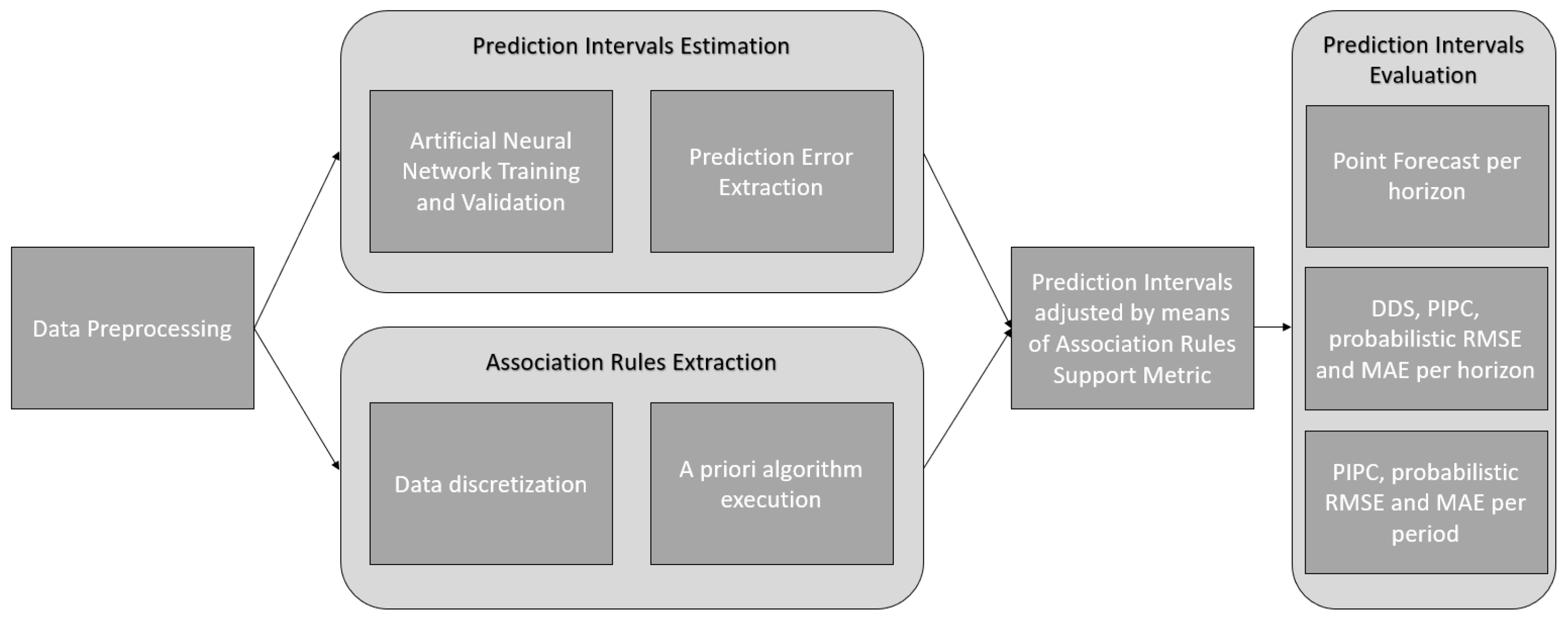
3. Materials and Methods

In this section, all the concepts of the developed methodology are described. First, there is a data preprocessing stage in which the raw data is transformed to be used by machine learning algorithms. Specifically, in this step time series data is transformed into a tabular form in which every element of the table is a segment of the original time series. Also, every element of the table is paired with its correspondent time period. Then, point forecast and prediction interval estimation are performed using artificial neural network (ANN) models. Specifically, the ANN models perform point forecasts in a test database and every error is stored. The stored errors are used to estimate the prediction intervals. At the same time, association-rule mining is performed to extract significant rules by means of the a priori algorithm. Then, the prediction intervals estimated with the Artificial Neural Networks models are adjusted by means of the obtained rules. Finally, the prediction intervals and its adjusted versions are evaluated. In Figure 1, the overarching methodology is shown.

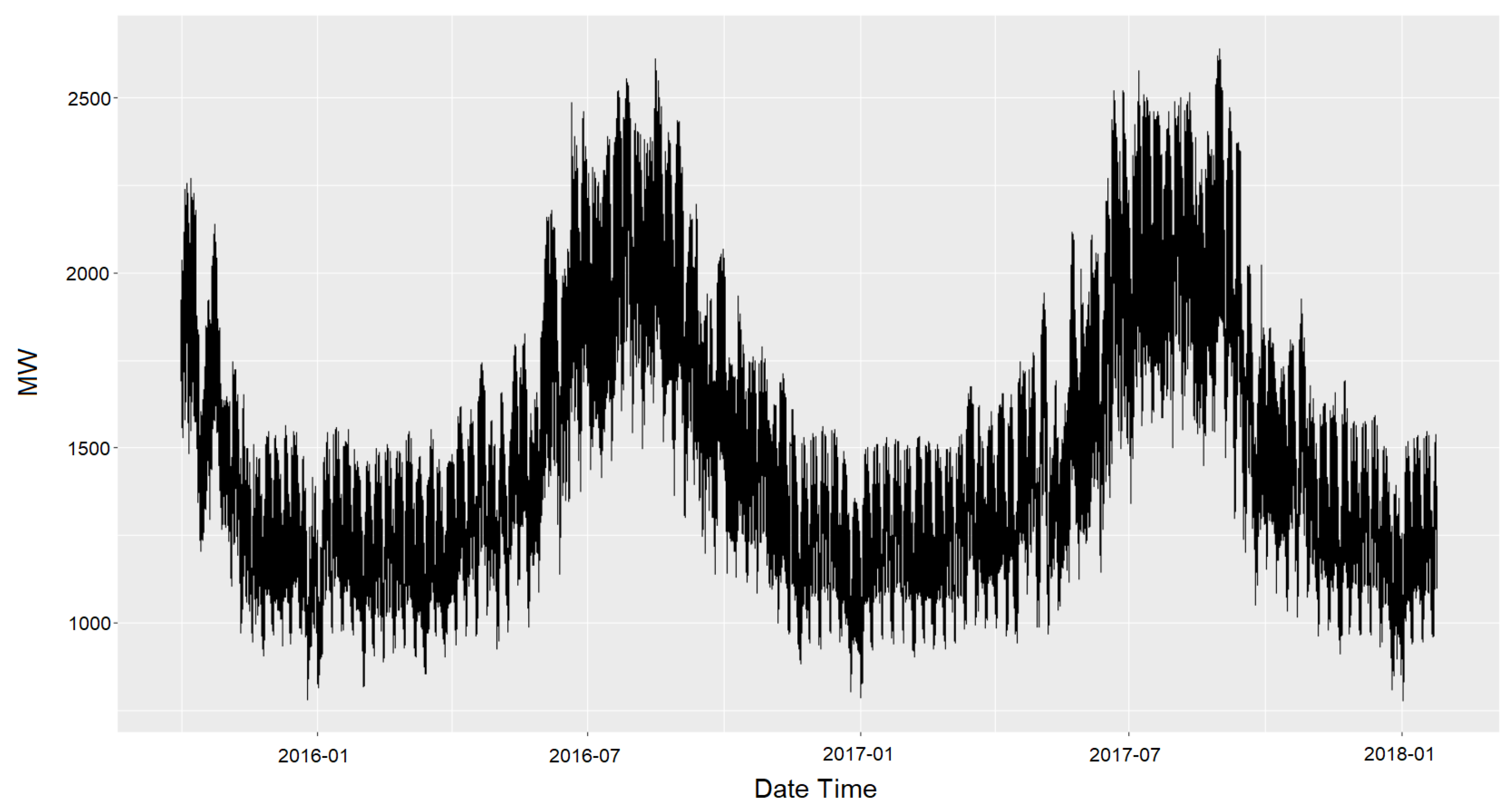
3.1. Data Preprocessing

The data are from a representative location of Mexico. The exact location of the data cannot be revealed due to confidentiality reasons. The data is composed of 15-min immediate measurements of load demand. This means that we have 96 periods of 15 min within a day. Also, that means that by the rules of the Mexican wholesale market, any prediction model bust be capable of predict 8 values in the future in 15 min interval (2 h ahead). In Figure 2, the graph of the complete data is shown.

To understand how the values distributed in the dataset, we use a histogram. In Figure 3, a graph of the histogram of the complete data is shown.

The complete dataset consists of 81,128 measurements from 1 October 2015, to 24 January 2018.

Table 1. Statistical properties of the dataset.

Name	Value
Minimum	779.2 MW
Median	1418.6 MW
Mean	1501.8 MW
Maximum	2641.0 MW

gives a summary of the statistical properties of the data.

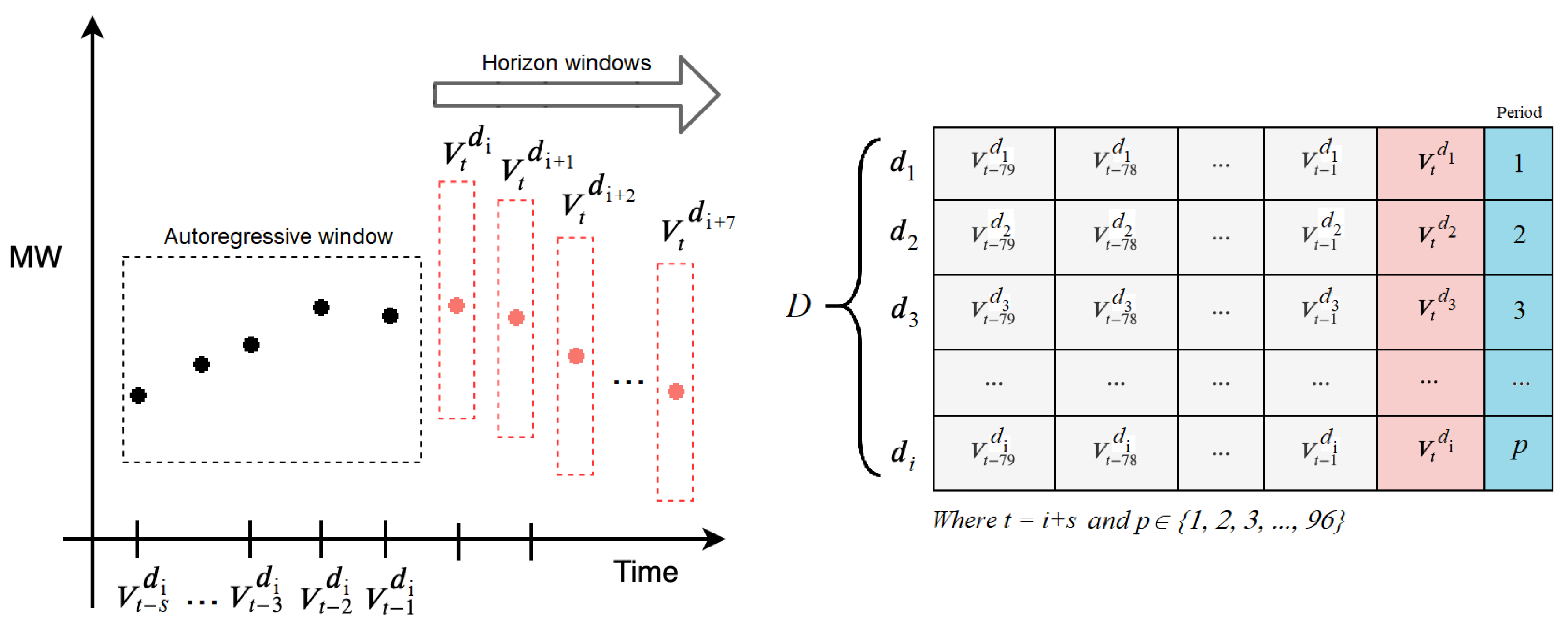
3.1.1. Load Data Embedding

For preprocessing, the time series is ordered in a form of delay embedding. The selected number of periods for the delay embedding is represented by s. For this paper, s is selected by the thumb rule described in [20]. The thumb rule states that for autoregressive models, at least 50 but preferably more than 100 observations should be taken. Based on this thumb rule, we decided to select 10 times the horizons h needed for this problem (8 horizons). Therefore, every example is conformed by vectors of 80 values, in which the last value is considered to be the dependent variable described by the rest of autoregressive values. Thus, for this paper $s=79$. The final objective is to transform the original time series dataset into a table form. To achieve this transformation, the set of delayed time series is constructed as follows:

Let L be set of load measurements:

$$L=\{V_1,V_2,\dots ,V_n\}$$

(1)

where n is the number of observations.

Let D be the set of delayed time series:

$$D=\{d_1,d_2,\dots ,d_m\}$$

(2)

where $m=n-s$ and $d_i$ is defined as follows:

$$d_i=\{V_j\in L|j\in \{t-s,\dots ,t-2,t-1,t\}\}$$

(3)

where $t=i+s$.

In summary, the constructed dataset D contains m delayed time series $d_i(i\in \{1,2,\dots ,m\})$, and every delayed time series $d_i$ contains values of the L dataset in the form of $\{V_{t-s},\dots ,V_{t-2},V_{t-1},V_t\}$ where $t=i+s$. It is important to note that every $d_i$ is distinct because of $t=i+s$, which means that even if every $d_i$ is constructed by $\{V_{t-s},\dots ,V_{t-2},V_{t-1},V_t\}$ values, t is different for every $d_i$. In Figure 4, an example of a d delayed time series is shown.

For every $d_i$, $V_t$ represents the dependent variable and $\{V_{t-s},\dots ,V_{t-2},V_{t-1},V_t\}$ the independent variables. Also, every $d_i$ is paired to its correspondent period $p\in \{1,2,\dots ,96\}$. This pairing allows applying machine learning algorithms in subsets defined by each period. Specifically, in the case of Association Rules, it is necessary to apply a discretization method, albeit the format is essentially the same. In Section 3.3.1, this discretization process is explained. In the next section, the process of prediction interval estimation through artificial neural networks is explained.

3.2. Prediction Interval Estimation

A prediction interval (PI) is the estimation of a range in which a load value will fall with a certain probability [21]. PI estimation is an important part of a forecasting process and it is intended to indicate the expected uncertainty of a point forecast. Also, PIs allows us to offer a set of values in which a future value will fall given a probability, thus, creating a probabilistic forecast result. The following is a general form of a $100(1-\alpha )\%$ confidence prediction interval expression:

$$\widehat{V_t}(p,h)\pm z_{\alpha }\sqrt{Var\left[ϵ\right(p,h\left)\right]}$$

(4)

where $\widehat{V_t}(p,h)$ is the point forecast of the period p in the horizon h, $z_{\alpha }$ is the z-$score$ of an empirical distribution given the probability $100(1-\alpha )\%$ and $ϵ(p,h)$ is the empirical distribution of errors of the forecast method in the period p and horizon h. In Equation (4), the z-$score$ is the parameter that allows us to modify the prediction interval coverage [22]. In Figure 5, an example of how the z-$score$ modifies the prediction interval coverage.

It is worth mentioning that z-$score$ value depends on the $\alpha$ value. Specifically, z-$score=Z\left(100\right(1-\alpha \left)\right)$ where Z is a function that estimates the z-$score$ value.

Prediction interval estimation using Equation (4) requires estimation of a set of prediction errors of a forecast model. In this paper, we use Artificial Neural Networks to generate a prediction model for each period of p.

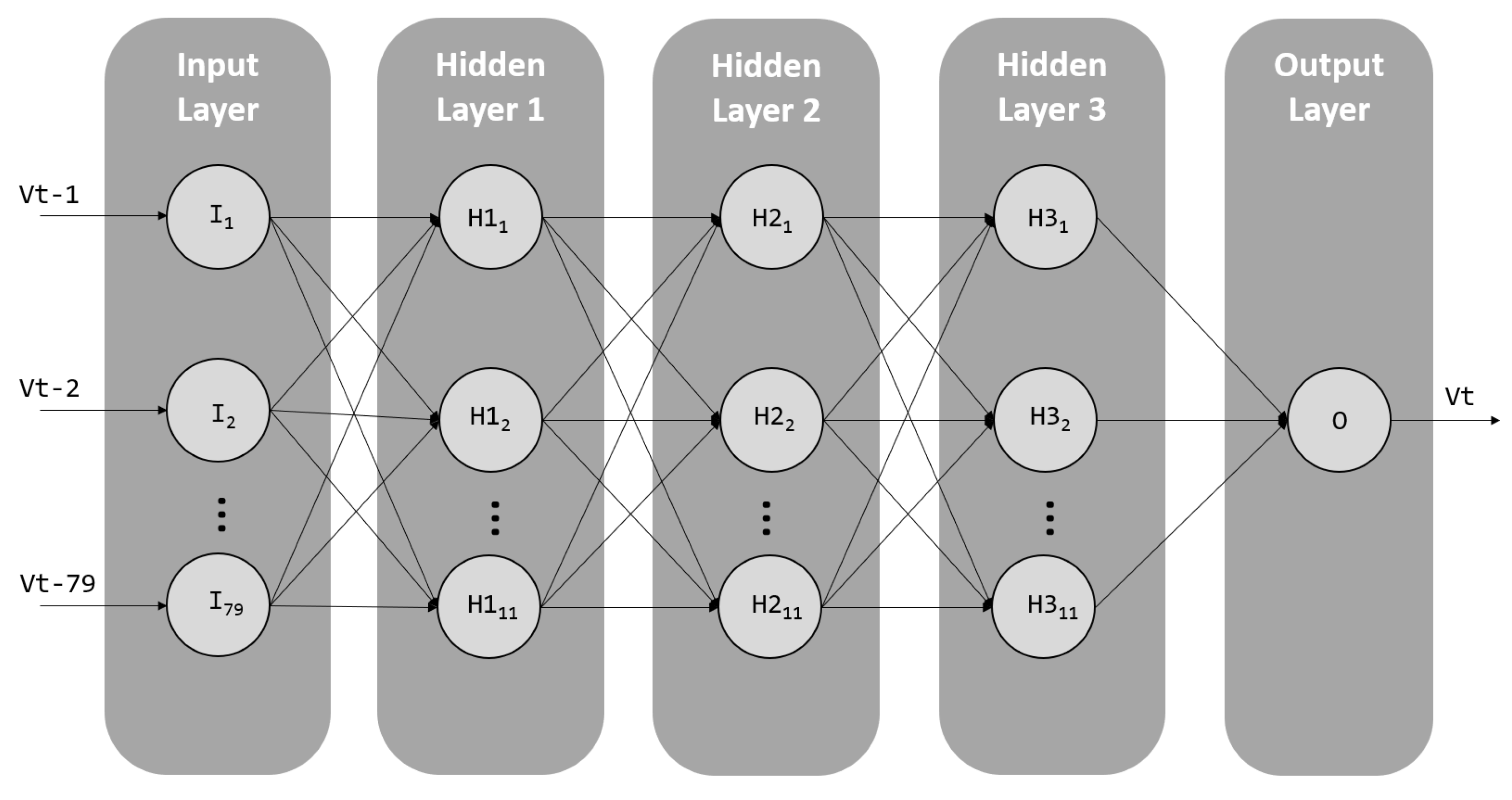
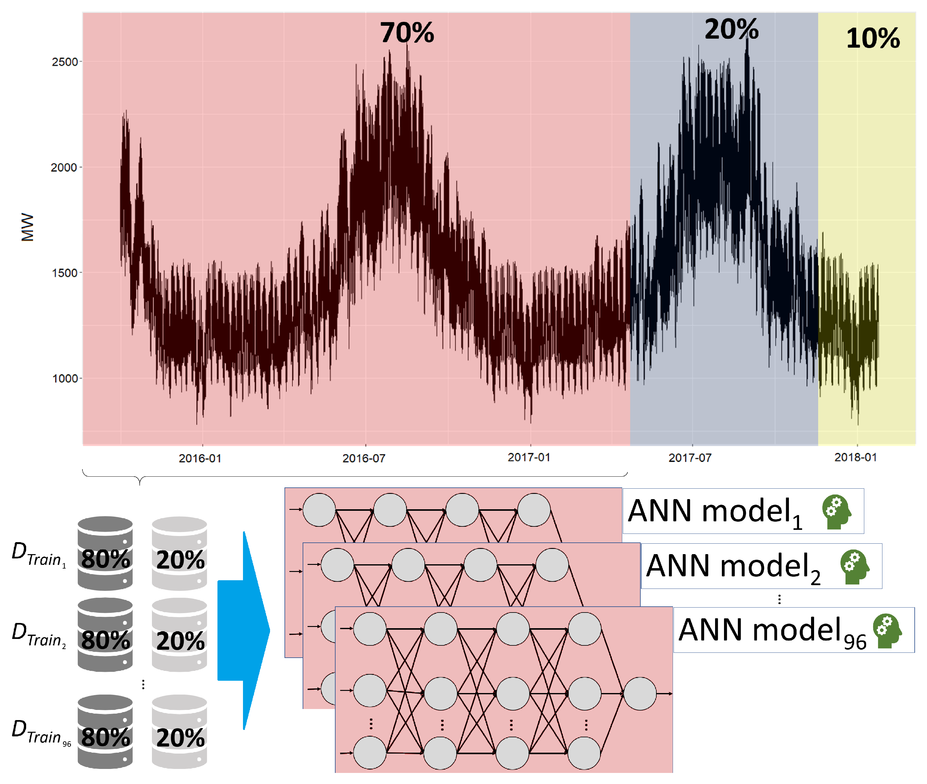
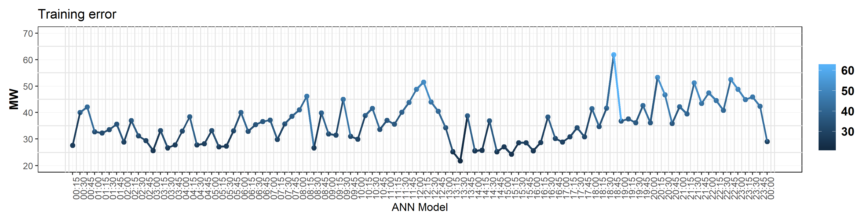
3.2.1. Artificial Neural Network Training and Validation

Artificial Neural Networks (ANN) are models inspired by the central nervous system, which are made of interconnected neurons [23]. One of the most common ANN paradigms for both classification and regression is the Multi-Layer Perceptron (MLP). An MLP artificial neural network is composed of multiple layers of neurons: an input layer, one or more hidden layers, and an output layer. The input layer is responsible for receiving a given input vector and transform it into an output that becomes the input for another layer. A hidden layer transforms the output from the previous layer through a transfer function. Each neuron receives the input from all the neurons in the preceding layer, multiplies each input by its corresponding weight vector and then adds a bias. In this paper, a 3-hidden layer with 11 neurons per layer ANN was implemented.

We selected 3 hidden layers employing a rule described in [24] and then updated in [25]. The rule indicates that for complex problems, such as time series prediction and computer vision, 3 or more layers are adequate. Also,  [24] states three rules to select the number of hidden neurons, for our problem we selected the rule that establishes the number of hidden neurons as 2/3 of the number of the input neurons. Thus, the number of hidden neurons would be $(79/3)\times 2\approx 52$ neurons (17 neurons per layer.). However, in [24] they warn that too many neurons per layer may lead to overfitting, so we still tried to reduce the number of hidden neurons and tested architectures from 17 to 10 neurons per layer, 11 neurons per layer was the one architecture to have similar error rate as 17 neurons per layer in terms of MAE (Means Absolute Error).

The method for training the ANN models in this paper is the Resilient Backpropagation method described in [26]. Regarding the activation function, despite the existence of several types of activation functions such as linear, tanh, gaussian, etc. the sigmoidal function is conventionally used in time series forecasting, hence, the latter was employed [27]. In Figure 6, a graphical representation of this configuration is shown.

To train the ANN models, create the prediction intervals, and test the prediction intervals, the total dataset D was divided into three groups: $D_{Train}$, $D_{TrainPI}$ and $D_{Test}$. $D_{Train}$ is composed of the first 70% of data, $D_{TrainPI}$ of the following 20% $D_{Test}$ of the last 10%. $D_{Train}$ is divided in 96 subsets in a 80% train-20% test format. The elements contained in every $D_{Train}$ subdivision are sorted randomly. The subdivided $D_{Train}$ is used to train an ANN model a per subdivision. As a result, 96 ANN models were obtained and stored in a dataset A$(a_p\in A|p\in \{1,2,\dots ,96\})$. In Figure 7, a graphical representation of the Artificial Neural Networks models training is shown.

In Figure 8, a graphical representation of the training error per ANN model is shown. In the x axis of the graph, every model is represented with its correspondent time period.

Once the ANN models were obtained, we proceed to extract the prediction errors using $D_{TrainPI}$. The following section explains this process.

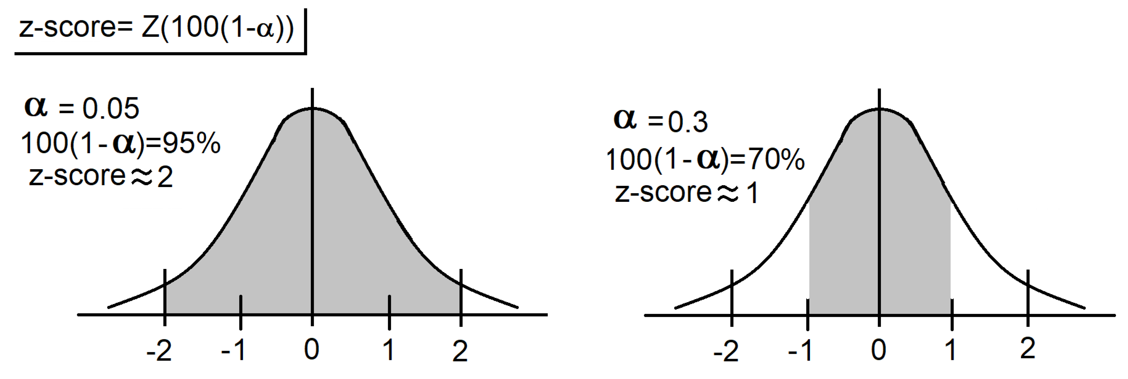
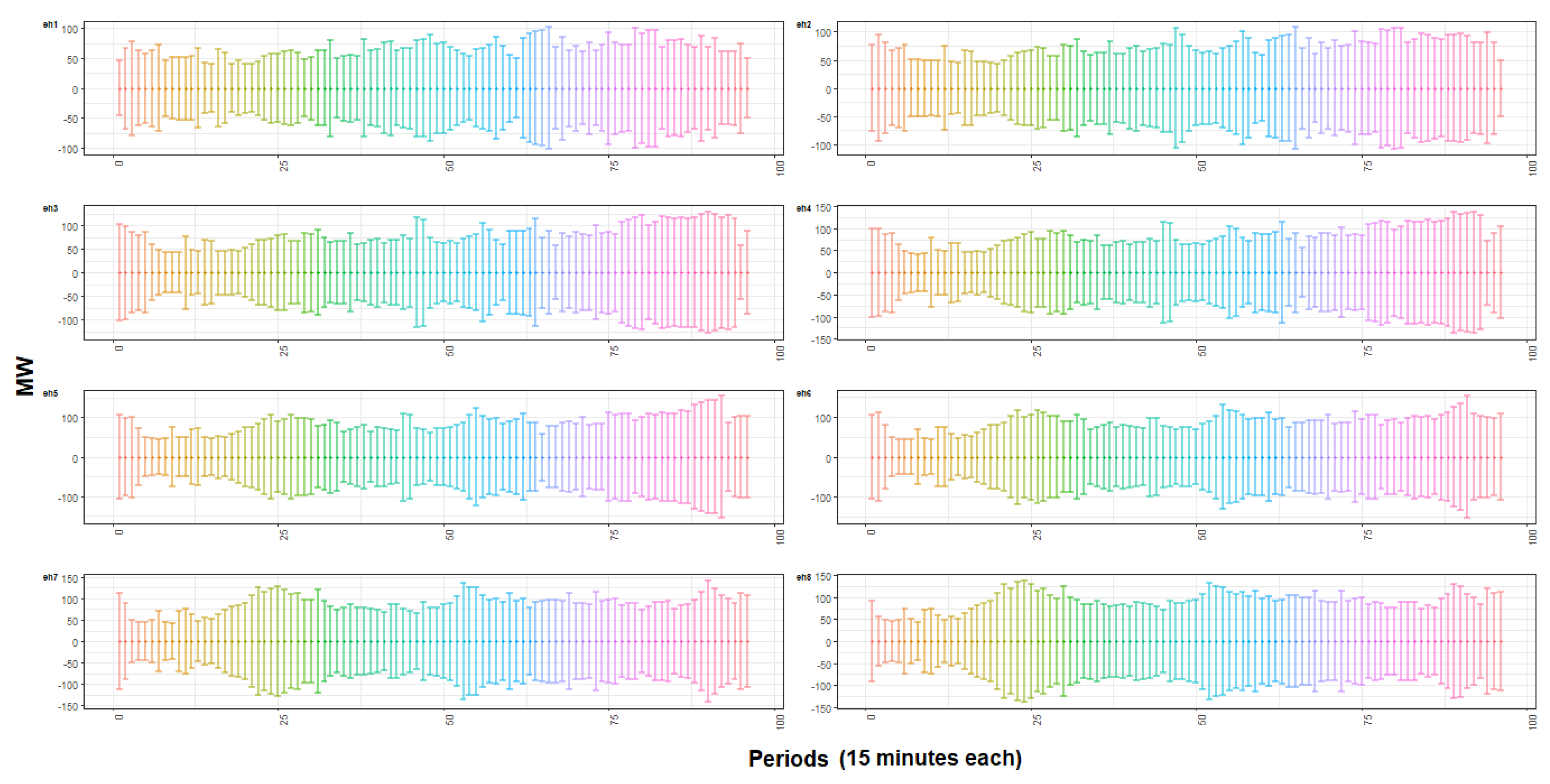
3.2.2. Prediction Error Extraction

For prediction error extraction, the obtained ANN models are used to predict the $V_t$ values contained in $D_{TrainPI}$. The ANN models takes the values of $W_i=\{V_{t-s},\dots ,V_{t-2},V_{t-1},V_t\}$ as inputs and produces $\widehat{V_t}(p,h)$ as output. Every measured error is stored in a separate database ($D_{ϵ}$). The obtained ANN models are purposely trained to predict only 1 horizon ahead (this to get 96 specialists ANN models in its correspondent period). Therefore, to predict the 8 horizons h needed for our problem, we use the predictions of the previous models of the last horizon as inputs, thus, $D_{ϵ}$ contains a set of $ϵ(p,h)$ prediction errors for every period p for each horizon h. For every $ϵ(p,h)$, the $\sqrt{Var[{ϵ}_{(}p,h)]}$ value is estimated to obtain the final prediction interval per horizon and per period. In Figure 9 a series of graphs of the obtained prediction intervals are shown.

We call these prediction intervals the normal prediction intervals. Normal prediction intervals are used in conjunction with the support values of the association rules method to construct the Adjusted prediction intervals. In the next section, the extraction of association rules from the dataset is explained.

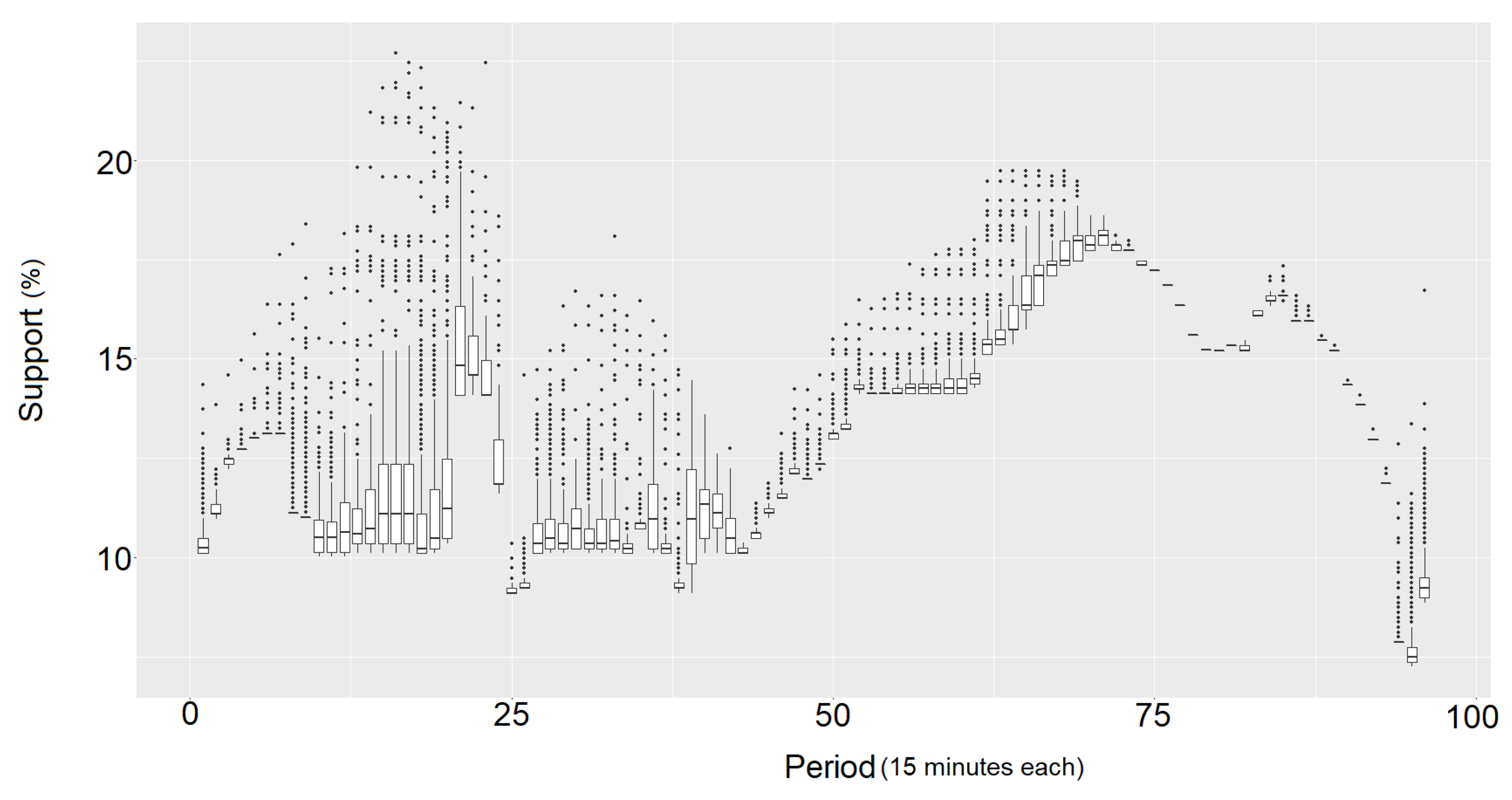
3.3. Association Rules Extraction

Association rules is a data mining methodology to extract relationships and dependencies between variables in datasets [28]. Its objective is to identify if-then patterns which are discovered in databases using some measures of interest [29]. For this paper, the a priori algorithm (see Appendix A and Appendix B) is used to extract the rulesets needed.

3.3.1. Data Discretization

Numeric data is difficult to use in the a priori algorithm, so a discretization method is needed. In this paper, the discretization of data is made through the method described in [30], specifically, the type 7 quantile method. The discretization method is carried out as follows:

Let $Q_7\left(P\right)$ be the type 7 quantile of the probability $P\in \{0.1,0.2,\dots ,1\}$:

$$Q_7\left(P\right)=(1-\gamma )·x_{\left(j\right)}+\gamma ·x_{(j+1)}$$

(5)

where $x_{\left(j\right)}$ is the jth order statistic of x, n is the sample size, $j=⎣n·P+m⎦$ and $\gamma =n·P+m-j$ and $m=1-P$. In this paper, $X=\{d_1\cup V_t|V_t\in d_i;i\in \{2,3,\dots ,m\}\}$. Using Equation (5) in the set X, we can obtain the bins for data discretization. In 

Table 2. Quantiles obtained using Equation (5).

0%	10%	20%	30%	40%	50%	60%	70%	80%	90%	100%
779	1079	1178	1273	1353	1418	1508	1631	1810	2088	2641

, the obtained bins and quantiles are shown.

The last row of Table 2 indicates the bins correspondent to the quantiles above them. Specifically, above every Bin, there is its lower and upper limit. Every value of set X is mapped according to its correspondent bin, so if a value falls inside the range of a bin, that value is substituted with the bin number and stored in a dataset $L^{\ast }$. Therefore, using the dataset $L^{\ast }$ we can construct the transactional dataset $D_{Trans}$ as follows:

Let $L^{\ast }$ be set of quantile mapped load measurements:

$$L^{\ast }=\{V_1^{\ast },V_2^{\ast },\dots ,V_{n^{\ast }}^{\ast }\}$$

(6)

where $n^{\ast }$ is the number of observations in $L^{\ast }$.

Let $D_{Trans}$ be the set of delayed of the quantile mapped time series:

$$D_{Trans}=\{d_1^{\ast },d_2^{\ast },\dots ,d_{m^{\ast }}^{\ast }\}$$

(7)

where $m^{\ast }=n^{\ast }-s$ and $d_i^{\ast }$ is defined as follows:

$$d_i^{\ast }=\{V_j^{\ast }\in L^{\ast }|j\in \{t-s,\dots ,t-2,t-1,t\}\}$$

(8)

where $t=i+s$.

For every $d_i^{\ast }$, $r_i^{\ast }=V_t^{\ast }$ represents the right part of the rule, and $l_i^{\ast }=\{V_{t-s}^{\ast },\dots ,V_{t-2}^{\ast },V_{t-1}^{\ast }\}$ represents the left part of the rule. Also, every $d_i^{\ast }$ is paired to its correspondent period $p\in \{1,2,\dots ,96\}$. The rule extraction process is carried out in $D_{Trans}$ using the a priori algorithm. In this paper, the parameters for the a priori algorithm are set so as obtaining rules with minimum $support=0.1$ and $confidence=0.9$ (In some periods where rules were not found, $support<0.1$ was used). The period element of the transactions dataset is used to segment the data into 96 subsets, one for every period. Then, the a priori algorithm is applied on each subset to obtain a ruleset $rs$ for every subset. As a result, 96 rulesets were obtained and stored in a dataset R$(r{s}_p\in R|p\in \{1,2,\dots ,96\})$. In Figure 10, a graph of the distribution of the support value per period is shown. Every period distribution is represented as a box plot in which inside the box there is the 95% of the support values in period p.

The process of prediction interval adjustment using the rulesets contained in R is explained in the next section.

3.4. Prediction Intervals Adjusted by Means of Association Rules Support Metric

The prediction interval is adjusted by subtracting the value of a correspondent rule support to the $100(1-\alpha )\%$ value when estimating the prediction interval. This adjustment occurs only when a specific rule in $r_p$ matches with the inputs of a $a_p$ ANN model. In this case, Equation (4) can be re-written as follows:

$$\widehat{V_t}(p,h)\pm z_{\delta }\sqrt{Var\left[ϵ\right(p,h\left)\right]}$$

(9)

where $\delta =\alpha +\beta$

The parameter $\beta$ is a bias to adjust the value of the z-$score$. The modified z-$score$ will decrease or not the prediction interval. The parameter $\beta$ can take values according to the following expression:

$$\beta =\{\begin{array}{ccc}support(l_i^{\ast }\Rightarrow r_i^{\ast }),& \mathrm{if}& W_i^{\ast }=l_i^{\ast }\hfill \\ 0,& & \mathrm{Otherwise}\hfill \end{array}$$

(10)

where $W_i^{\ast }$ is the quantile mapped version of the ANN model inputs $W_i$. To modify the value of the z-$score$, we re-write the confidence interval probability expression as follows:

$$100·(1-(\alpha +\beta \left)\right)$$

(11)

From the modified confidence interval probability shown in Equation (11), we can obtain the modified prediction interval confidence. With this value, we can look forward to its corresponding modified z-$score$ from any z-$score$ table [22]. This, in fact, gives us the corresponding z-$score$ value, such that we can modify the coverage of the prediction interval.

4. Experiments and Results

To measure the efficiency of the prediction intervals (Normal and Adjusted), we propose the use of the Prediction Interval Coverage Probability (PICP) [31] and the Dawid–Sebastiani Score (DSS) [32]. We also measure probabilistic and point-forecast MAE and RMSE per horizon h and the PICP per period p for a better understanding of the prediction interval efficiency. To evaluate the quality of the Adjusted prediction interval, three experiments were conducted: All days, Weekdays and Weekends in dataset $D_{Test}$. For every experiment, normal prediction intervals (Normal) and Adjusted prediction interval (Adjusted) are evaluated. The process to implement these evaluations consists of three steps:

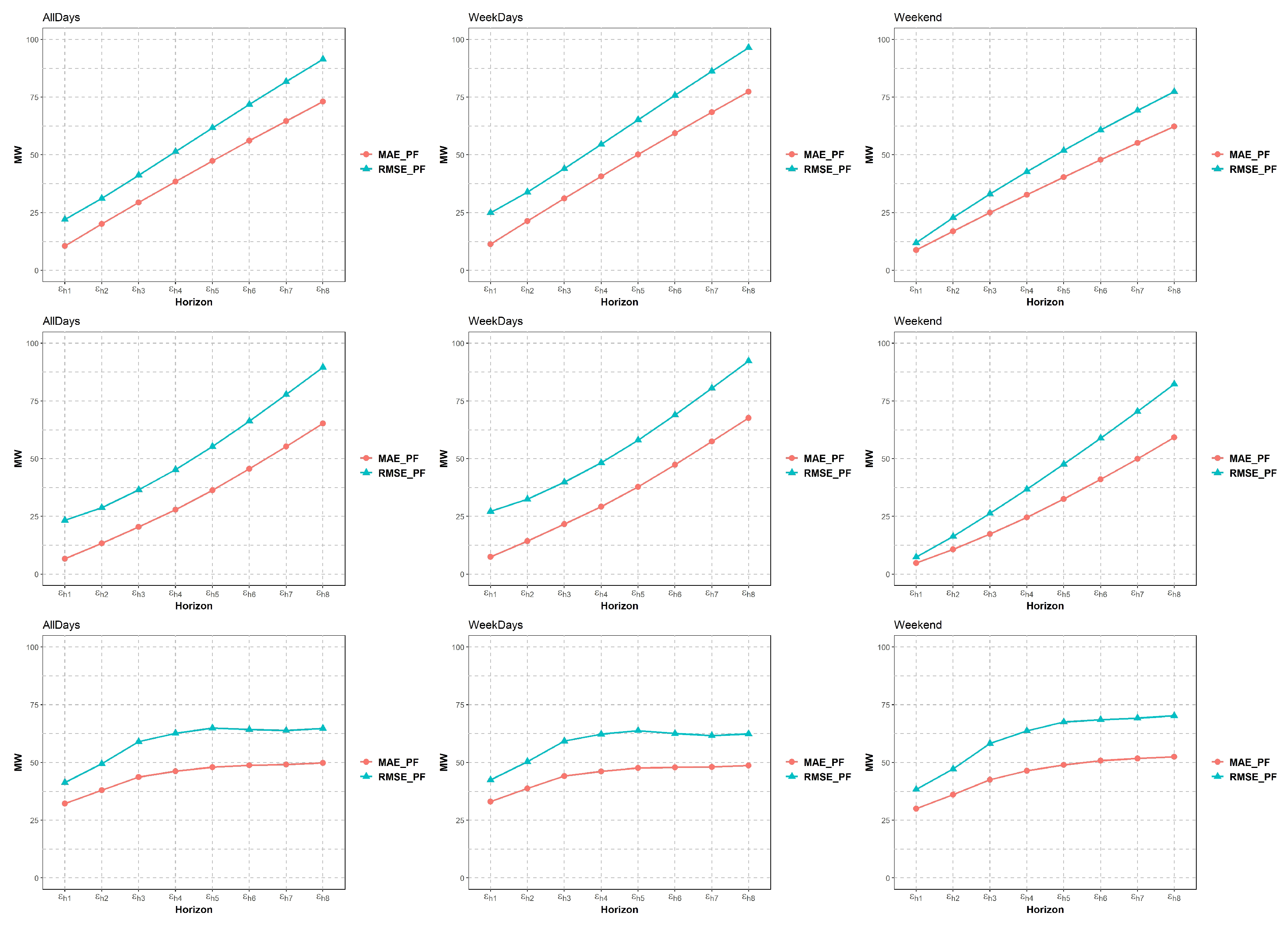
• Calculate Root Mean Squared Error (RMSE) and Mean Absolute Error (MAE) for the point forecasts for each horizon.
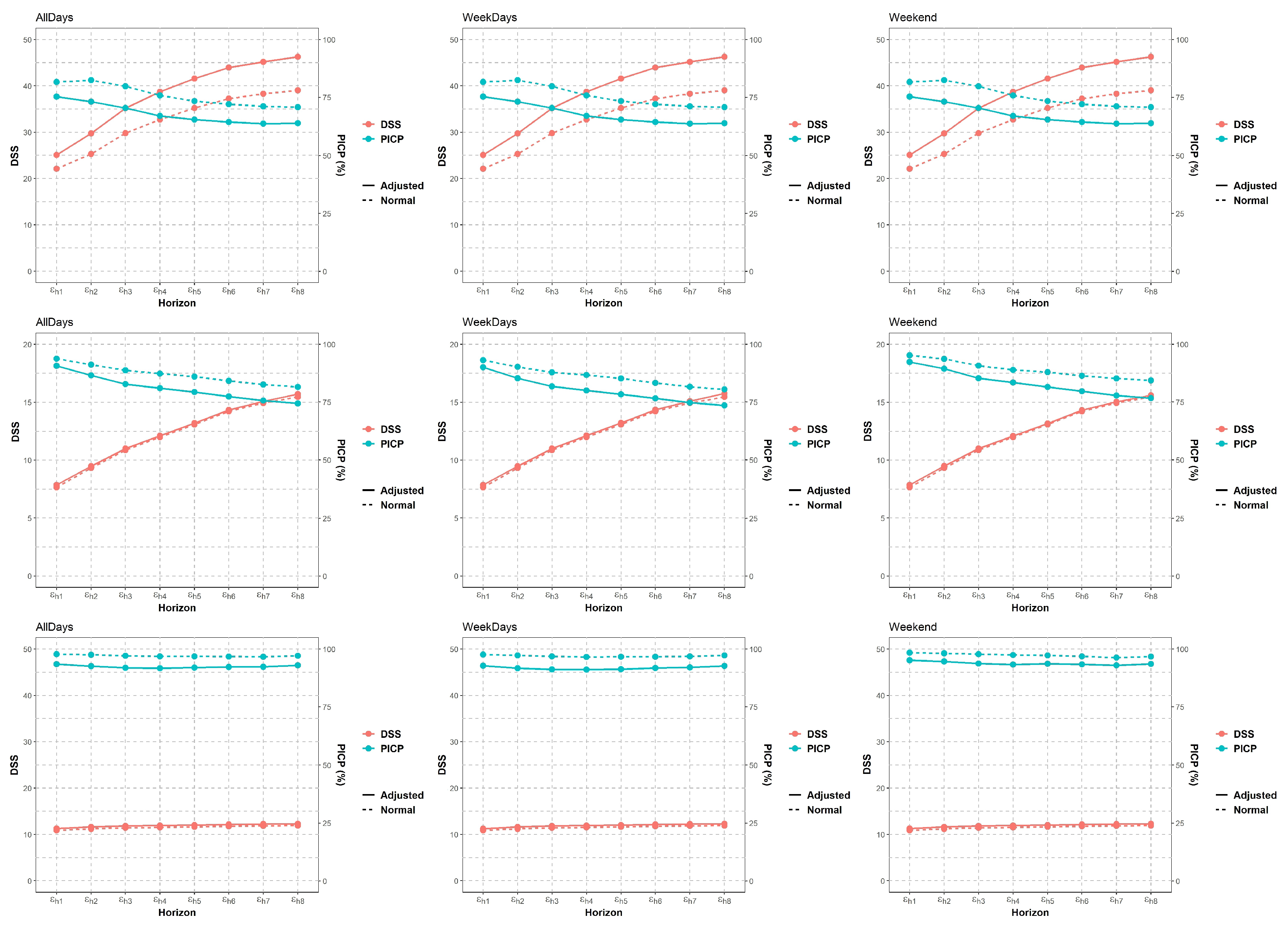
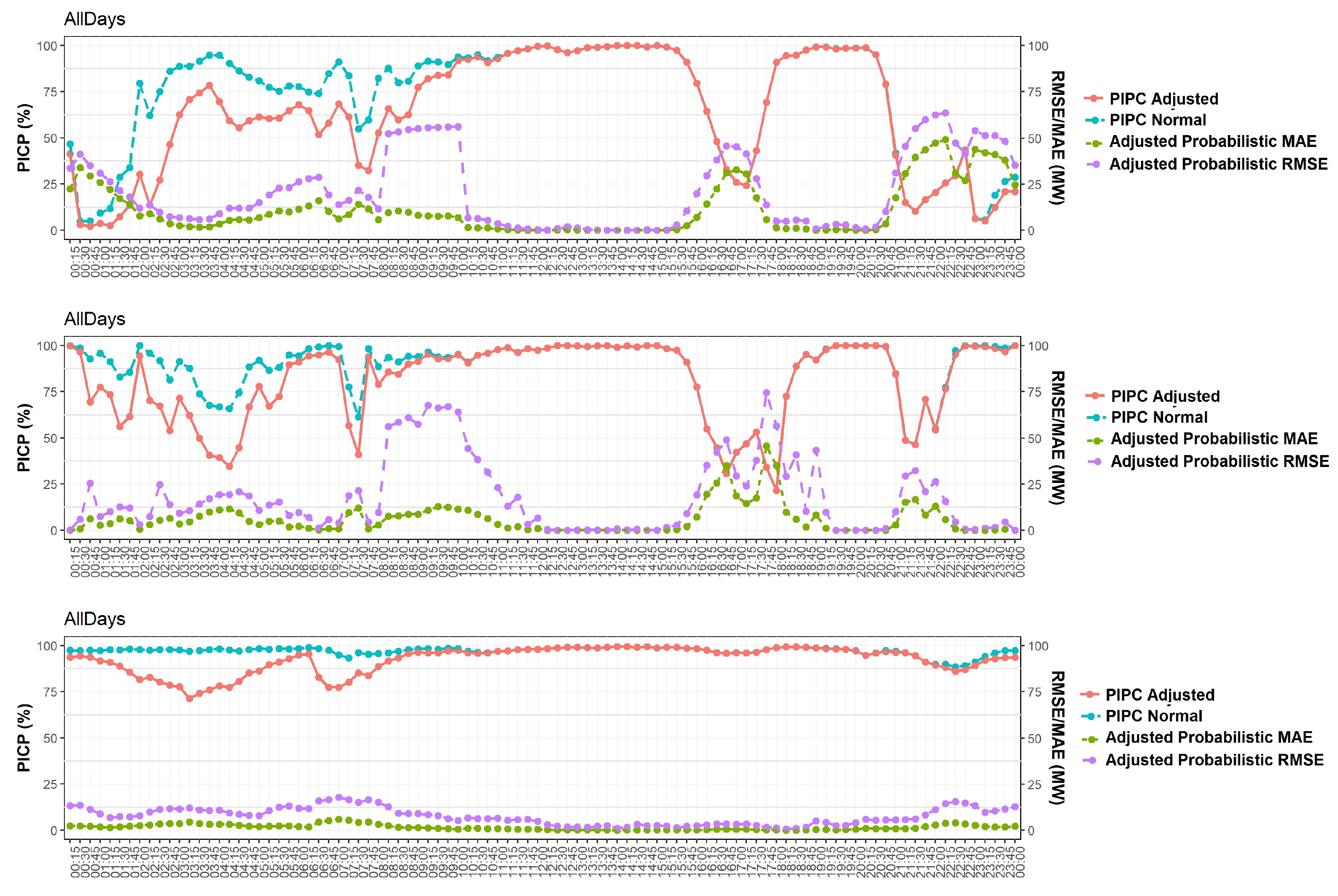
• Calculate the Dawid–Sebastiani score (DSS) and Prediction Interval Coverage Probability (PIPC) along with Probabilistic RMSE and MAE per horizon.
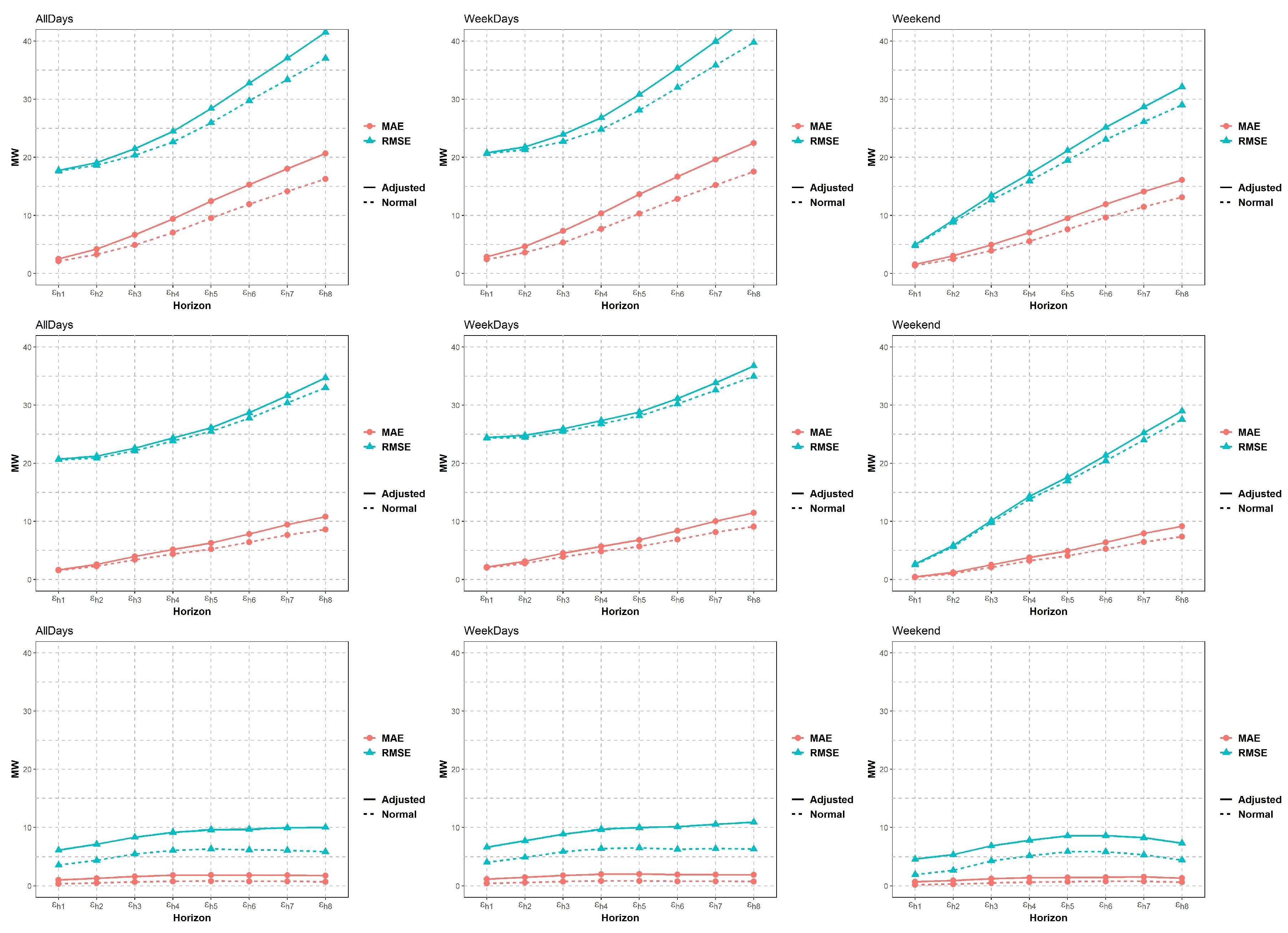
• Estimate PIPC and probabilistic RMSE and MAE of the Adjusted prediction interval per period.

In the following section, the implementation of the mentioned metrics is described.

4.1. Prediction Intervals Evaluation Metrics

In this section, prediction intervals evaluation metrics are described. These metrics are helpful to evaluate and understand both Normal and Adjusted prediction intervals.

4.1.1. PICP (Prediction Interval Coverage Probability)

The PICP is the rate of real values that lies within the prediction interval. The PICP is estimated using the following equation:

$$PICP=\frac{1}{w}·\sum _{g=1}^w{\theta }_g$$

(12)

where w is the number of observations and ${\theta }_g$ is defined by the following equation:

$${\theta }_g=\{\begin{array}{ccc}\hfill 1,& \mathrm{if}& V_t(p,h)<U(p,h)\mathrm{and}{V}_t(p,h)>L(p,h)\hfill \\ \hfill 0,& & \mathrm{Otherwise}\end{array}$$

(13)

where $U(p,h)=\widehat{V_t}(p,h)+z_{\delta }\sqrt{Var\left[ϵ\right(p,h\left)\right]}$ and $L(p,h)=\widehat{V_t}(p,h)-z_{\delta }\sqrt{Var\left[ϵ\right(p,h\left)\right]}$.

4.1.2. Probabilistic and Point-Forecast RMSE (Root Mean Squared Error) and MAE (Mean Absolute error)

Probabilistic and point-forecast error is measured as indicated in Figure 11. Point forecast corresponds to the predicted load value, Outside Prediction Interval stands for those load measures that fall above or below the prediction interval range, and Inside Prediction Interval corresponds to the actual load measure that falls inside of the prediction interval range.

Using all the errors, we estimate probabilistic and point-forecast MAE and RMSE using the respective set of errors. Point MAE and RMSE estimation help us to estimate the precision of the forecast method, also helps us to understand the prediction intervals in general. Probabilistic MAE and RMSE help us to understand better the PICP metric result.

4.1.3. DSS (Dawid–Sebastiani Score)

The Dawid–Sebastiani Score (DSS) helps us to understand the quality of the prediction interval. The DSS is estimated as indicated in the following equation:

$$DSS={\left(\frac{{ϵ}_k-E\left[ϵ(p,h)\right]}{{\sigma }_{ϵ(p,h)}}\right)}^2+2·log\left({\sigma }_{ϵ(p,h)}\right)$$

(14)

where ${ϵ}_k$ and ${\sigma }_{ϵ(p,h)}$ are the kth error and the standard deviation from the error distribution $ϵ(p,h)$ respectively. Equation (14) is modified to estimate the DDS of the Adjusted prediction intervals based on the support of the rules. The following equation describes the modified version of the DSS:

$$DSS={\left(\frac{{ϵ}_k-E\left[ϵ(p,h)\right]}{{\sigma }_{ϵ(p,h)}·(1-E\left[supp(p,h)\right])}\right)}^2+2·log({\sigma }_{ϵ(p,h)}·(1-E\left[supp(p,h)\right]))$$

(15)

where $supp(p,h)$ is the set of support values used to adjust prediction intervals in period p and horizon h. It is worth mentioning that if no interval were modified, then $supp(p,h)$ will be filled with $0^{\prime }s$ and Equation (15) will become (14).

4.2. Results and Discussion

To compare the proposed approach, the Autoregressive Integrated Moving Average (ARIMA) model and a persistence model are also evaluated. The ARIMA model is a classical time series forecasting method. This method depends on three parameters: p which stands for the number of autoregressive variables; q which refers to the number of moving average variables; and d which indicates the number of times the data needs to be differentiate such that the time series is stationary. For experimental purposes, we estimated the ARIMA model using the process one described in [33]. The persistence model is often used to know if a forecast model provides better results than any trivial reference model [34]. First, we present the point-forecast MAE and RMSE. Whereas point-forecast MAE gives us a general idea of the precision of the forecast model, point-forecast RMSE penalizes large errors, so if the ANN models tend to return large error values the RMSE will be greatly separated from point-forecast MAE. In Figure 12, the point-forecast MAE and RMSE for the Persistence, ARIMA and the proposed model are shown.

As we can observe in Figure 12, the persistence and the ARIMA models work better, for point forecasts, in the first 5 horizons in comparison to the proposed model. However, the proposed model point-forecast RMSE follows the same tendency as point-forecast MAE, so we can say that the errors are consistent along the horizons for the three experiments, unlike the ARIMA and the persistence model for which the errors are larger along the horizons. Although we can observe that errors are consistent along the horizons for the proposed model, we can also observe that point-forecast MAE and RMSE tends to be larger in the Weekend experiment for the three models. This behavior is expected as we suppose that human activities in the Weekend are less constant than Weekdays. Then we present the DSS and the PICP along with the probabilistic MAE and RMSE. These results are presented per horizon and for all the three experiments and the three models evaluated. In Figure 13, the result of the DDS and the PICP per horizon is shown.

As we can observe in Figure 13, the DSS for the ARIMA and the persistence model is larger than the measurement of the proposed model for both Adjusted and Normal prediction intervals (larger values of DSS indicates lower quality of prediction intervals). Also, we can observe that the PIPC for the ARIMA and the persistence model is lower than the measurement of the proposed model for both Adjusted and Normal prediction intervals. For ARIMA and the proposed model, DSS and PICP per horizon of Adjusted and Normal prediction intervals are really close along the horizons for the three experiments, which indicates that for those models, the Adjusted and Normal prediction intervals are quite similar. Probabilistic MAE and RMSE provide another perspective of this result. In Figure 14, probabilistic MAE and RMSE for the persistence, ARIMA, and the proposed model is shown.

As we can observe in Figure 14, for ARIMA and the persistence model the probabilistic MAE and RMSE are larger than the proposed model, and also that is increasing along the horizons. Although probabilistic MAE and RMSE for ARIMA and the persistence model are quite similar between Adjusted and Normal prediction intervals, probabilistic RMSE value is much separated from probabilistic MAE, which indicates that errors are very large sometimes.

For the proposed model, probabilistic MAE indicates that Adjusted prediction intervals fail by less than 2.5 MW along the horizons, which is not significant if we compare it to the 1.3 MW the Normal prediction interval failure. Also, probabilistic RMSE shows that the probabilistic error tends to be larger than MAE along the horizons, but the maximum difference between Adjusted and Normal probabilistic RMSE is less than 6 MW, which is also not significant. This significance is measured by the ancillary services requirements [35]. Ancillary services requirements are published daily in the Independent System Operator official site. For the region this method is applied, the requirements of the ancillary services for the first horizon is a constant value of 25 MW. This means that errors below 25 MW do not affect the power systems significantly. Also, it is worth mentioning that probabilistic MAE and RMSE are smaller in the Weekend experiment. This behavior may happen point-forecast RMSE and MAE are larger in the Weekend experiment, so we can expect prediction intervals to be larger on Weekends. In general, we can observe that the error metrics of the Adjusted prediction intervals are similar to the Normal prediction intervals. To understand better this similarity, we make use of PICP per period. In Figure 15 the PICP per period for all the three experiments and the three models is shown.

As we can observe in Figure 15, for the ARIMA and the persistence models, Normal and Adjusted PIPC are similar. However, we can also observe that RMSE and MAE are larger than the measured for the proposed approach. Also, it is interesting to observe that ARIMA and persistence models have larger errors in the periods of 08:00–12:00 and 15:45–19:00, this may be caused by the load change during the day with respect to the sun position. Also, it is interesting to observe that these errors are lower in the persistence model for the periods 15:45–19:00. For the proposed approach, we can observe that probabilistic MAE and RMSE are more stables along the periods than the measured of the ARIMA and the persistence model. Also, we can observe that although Adjusted PICP drops until less than 75%, probabilistic MAE indicates that the error is always less than 5 MW, which is not significant. Also, probabilistic RMSE shows that in most of the periods the error is less than 15 MW, which is also not significant. A prediction interval creation method is presented. The proposed approach for the creation of the prediction interval allows modifying the prediction interval by means of an association rules method. Using the proposed approach, the prediction interval can be reduced as much as the corresponding support value. We construct prediction intervals using Artificial Neural Network models and we adjust them by means of rules obtained with the a priori algorithm. Prediction interval quality and effectiveness are measured by means of Prediction Interval Coverage Probability (PICP) and the Dawid–Sebastiani Score (DSS). PICP and DSS per horizon show that the Adjusted and Normal prediction intervals are pretty similar. The proposed approach was compared to the ARIMA model and a persistence model. The proposed model demonstrates to have better performance in all the prediction interval evaluation metrics. Also, probabilistic and point-forecast MAE and RMSE metrics are used. Probabilistic MAE indicates that Adjusted prediction intervals fail by less than 2.5 MW along the horizons, which is not significant if we compare it to the 1.3 MW the Normal prediction interval failure. Also, probabilistic RMSE shows that the probabilistic error tends to be larger than MAE along the horizons, but the maximum difference between Adjusted and Normal probabilistic RMSE is less than 6 MW, which is also not significant. This work was focused on the prediction interval adjustment, so as future work we will use an optimization method to select the optimal structure of the ANN models per period with the objective of increasing accuracy of the ANN models prediction. For the association rules method, the discretization method will be modified to obtain more quantiles so the rules can be more specific. Also, we will relax the parameters of Support and Confidence to enlarge the diversity of rules, and at the same time, we will include the Confidence metric to the prediction interval adjustment. Finally, this method will be tested in another dataset such as ERCOT or the GefCom(2012, 2014, 2017).

References

1. Oconnell, N.; Pinson, P.; Madsen, H.; Omalley, M. Benefits and challenges of electrical demand response: A critical review. Renew. Sustain. Energy Rev. 2014, 39, 686–699. [Google Scholar] [CrossRef]
2. Alfares, H.K.; Nazeeruddin, M. Electric load forecasting: Literature survey and classification of methods. Int. J. Syst. Sci. 2002, 33, 23–34. [Google Scholar] [CrossRef]
3. Fan, S.; Hyndman, R.J. Short-term load forecasting based on a semi-parametric additive model. IEEE Trans. Power Syst. 2012, 27, 134–141. [Google Scholar] [CrossRef] [Green Version]
4. SENER; Secretaría de Energía (MX). Acuerdo por el que se emite el Manual de Mercado de Energía de Corto Plazo; Published Reform in 2016-06-17 Second Section; Diario Oficial de la Federación (DOF): Ciudad de México, México, 2016; pp. 10–76. [Google Scholar]
5. Raza, M.Q.; Khosravi, A. A review on artificial intelligence based load demand forecasting techniques for smart grid and buildings. Renew. Sustain. Energy Rev. 2015, 50, 1352–1372. [Google Scholar] [CrossRef]
6. Almeshaiei, E.; Soltan, H. A methodology for Electric Power Load Forecasting. Alex. Eng. J. 2011, 50, 137–144. [Google Scholar] [CrossRef] [Green Version]
7. Lee, D.; Park, Y.G.; Park, J.B.; Roh, J.H. Very short-Term wind power ensemble forecasting without numerical weather prediction through the predictor design. J. Electr. Eng. Technol. 2017, 12, 2177–2186. [Google Scholar]
8. Martínez-Álvarez, F.; Troncoso, A.; Asencio-Cortés, G.; Riquelme, J. A Survey on Data Mining Techniques Applied to Electricity-Related Time Series Forecasting. Energies 2015, 8, 13162–13193. [Google Scholar] [CrossRef] [Green Version]
9. Burda, M.; Štěpnička, M.; Štěpničková, L. Fuzzy Rule-Based Ensemble for Time Series Prediction: Progresses with Associations Mining. In Strengthening Links Between Data Analysis and Soft Computing; Springer International Publishing: Cham, Switzerland, 2015; Volume 315, pp. 261–271. [Google Scholar] [CrossRef]
10. Yadav, M.; Jain, S.; Seeja, K.R. Prediction of Air Quality Using Time Series Data Mining. In Opinion Mining of Saubhagya Yojna for Digital India; Springer: Singapore, 2019; Volume 55, pp. 13–20. [Google Scholar] [CrossRef]
11. Wang, C.; Zheng, X. Application of improved time series Apriori algorithm by frequent itemsets in association rule data mining based on temporal constraint. Evol. Intell. 2019. [Google Scholar] [CrossRef]
12. Gajowniczek, K.; Zabkowski, T. Data mining techniques for detecting household characteristics based on smart meter data. Energies 2015, 8, 7407–7427. [Google Scholar] [CrossRef] [Green Version]
13. Singh, S.; Yassine, A. Big Data Mining of Energy Time Series for Behavioral Analytics and Energy Consumption Forecasting. Energies 2018, 11, 452. [Google Scholar] [CrossRef] [Green Version]
14. Khosravi, A.; Nahavandi, S.; Creighton, D. Construction of optimal prediction intervals for load forecasting problems. IEEE Trans. Power Syst. 2010, 25, 1496–1503. [Google Scholar] [CrossRef] [Green Version]
15. Quan, H.; Srinivasan, D.; Khosravi, A.; Nahavandi, S.; Creighton, D. Construction of neural network-based prediction intervals for short-term electrical load forecasting. In Proceedings of the IEEE Symposium on Computational Intelligence Applications in Smart Grid (CIASG), Singapore, 16–19 April 2013; pp. 66–72. [Google Scholar]
16. Rana, M.; Koprinska, I.; Khosravi, A.; Agelidis, V.G. Prediction intervals for electricity load forecasting using neural networks. In Proceedings of the International Joint Conference on Neural Networks, Dallas, TX, USA, 4–9 August 2013. [Google Scholar]
17. Moulin, L.S.; da Silva, A.P.A. Neural Network Based Short-Term Electric Load Forecasting with Confidence Intervals. IEEE Trans. Power Syst. 2000, 15, 1191–1196. [Google Scholar]
18. Liu, H.; Han, Y.H. An electricity load forecasting method based on association rule analysis attribute reduction in smart grid. Front. Artif. Intell. Appl. 2016, 293, 429–437. [Google Scholar]
19. Chiu, C.C.; Kao, L.J.; Cook, D.F. Combining a neural network with a rule-based expert system approach for short-term power load forecasting in Taiwan. Expert Syst. Appl. 1997, 13, 299–305. [Google Scholar] [CrossRef]
20. Box, G.E.P.; Tiao, G.C. Intervention Analysis with Applications to Economic and Environmental Problems. J. Am. Stat. Assoc. 1975, 70, 70–79. [Google Scholar] [CrossRef]
21. Chatfield, C. Time-Series Forecasting, 1st ed.; Chapman and Hall/CRC: Boca Raton, FL, USA, 2000. [Google Scholar]
22. Hyndman, R.J.; Athanasopoulos, G. Forecasting: Principles and Practice, 2nd ed.; OTexts: Melbourne, Australia, 2018. [Google Scholar]
23. Hastie, T.; Tibshirani, R.; Friedman, J. The Elements of Statistical Learning; Springer Series in Statistics; Springer New York Inc.: New York, NY, USA, 2001. [Google Scholar]
24. Heaton, J. Introduction to Neural Networks for Java, 2nd ed.; Heaton Research, Inc.: Washington, DC, USA, 2008. [Google Scholar]
25. Jeff, H. The Number of Hidden Layers. Available online: https://www.heatonresearch.com/2017/06/01/hidden-layers.html (accessed on 21 August 2017).
26. Riedmiller, M. Rprop-Description and Implementation Details. Available online: http://www.inf.fu-berlin.de/lehre/WS06/Musterererkennung/Paper/rprop.pdf (accessed on 1 September 2017).
27. Chang, H.; Nakaoka, S.; Ando, H. Effect of shapes of activation functions on predictability in the echo state network. arXiv 2019, arXiv:1905.09419. [Google Scholar]
28. Agrawal, R.; Imieliński, T.; Swami, A. Mining Association Rules Between Sets of Items in Large Databases. SIGMOD Rec. 1993, 22, 207–216. [Google Scholar] [CrossRef]
29. Frawley, W.J.; Piatetsky-Shapiro, G.; Matheus, C.J. Knowledge Discovery in Databases—An Overview. Knowl. Discov. Databases 1992, 1–30. [Google Scholar] [CrossRef]
30. Hyndman, R.J.; Fan, Y. Sample Quantiles in Statistical Packages. Am. Stat. 1996, 50, 361–365. [Google Scholar]
31. Quan, H.; Srinivasan, D.; Khosravi, A. Uncertainty handling using neural network-based prediction intervals for electrical load forecasting. Energy 2014, 73, 916–925. [Google Scholar] [CrossRef]
32. Czado, C.; Gneiting, T.; Held, L. Predictive Model Assessment for Count Data. Biometrics 2009, 65, 1254–1261. [Google Scholar] [CrossRef] [PubMed]
33. Hyndman, R.J.; Khandakar, Y. Automatic Time Series Forecasting: The forecast Package for R. J. Stat. Softw. 2008, 27. [Google Scholar] [CrossRef] [Green Version]
34. Coimbra, C.F.; Pedro, H.T. Chapter 15—Stochastic-Learning Methods. In Solar Energy Forecasting and Resource Assessment; Kleissl, J., Ed.; Academic Press: Boston, MA, USA, 2013; pp. 383–406. [Google Scholar]
35. CENACE. Servicios Conexos. Available online: https://www.cenace.gob.mx/SIM/VISTA/REPORTES/ServConexosSisMEM.aspx (accessed on 30 November 2019).
Figure 1. The overarching methodology. PIPC: Prediction Interval Coverage Probability. DDS: Dawid-Sebastiani Score.
Applsci 09 05269 g001
Figure 2. Load time series measured every 15 min.
Applsci 09 05269 g002
Figure 3. The distribution of values in the whole dataset represented by means of an histogram.
Applsci 09 05269 g003
Figure 4. Graphical representation of a delayed time series.
Applsci 09 05269 g004
Figure 5. Prediction interval modification by means of the z- s c o r e .
Applsci 09 05269 g005
Figure 6. A graphical representation of the structure of the Artificial Neural Network used for this work.
Applsci 09 05269 g006
Figure 7. Graphical representation of the Artificial Neural Networks models training.
Applsci 09 05269 g007
Figure 8. Graphical representation of the Artificial Neural Networks models training.
Applsci 09 05269 g008
Figure 9. Graphs of the prediction intervals obtained.
Applsci 09 05269 g009
Figure 10. The support value distribution per period of the dataset to extract the rules.
Applsci 09 05269 g010
Figure 11. Probabilistic and point-forecast errors.
Applsci 09 05269 g011
Figure 12. Point-forecast MAE and RMSE for (from top to bottom) the persistence, ARIMA and the proposed model.
Applsci 09 05269 g012
Figure 13. DSS and PIPC corresponding to (from top to bottom) the persistence model, ARIMA, and the proposed model.
Applsci 09 05269 g013
Figure 14. Probabilistic MAE (Means Absolute Error) and RMSE (Root Mean Squared Error) for (from top to bottom) the persistence, ARIMA (Autoregressive Integrated Moving Average) and the proposed model.
Applsci 09 05269 g014
Figure 15. PICP comparison of Normal vs Adjusted prediction intervals, and probabilistic MAE/RMSE for the Adjusted prediction intervals per period.
Applsci 09 05269 g015