Multiscale Damage Evolution Analysis of Aluminum Alloy Based on Defect Visualization


Abstract
Featured Application
Abstract
1. Introduction
2. Experiment
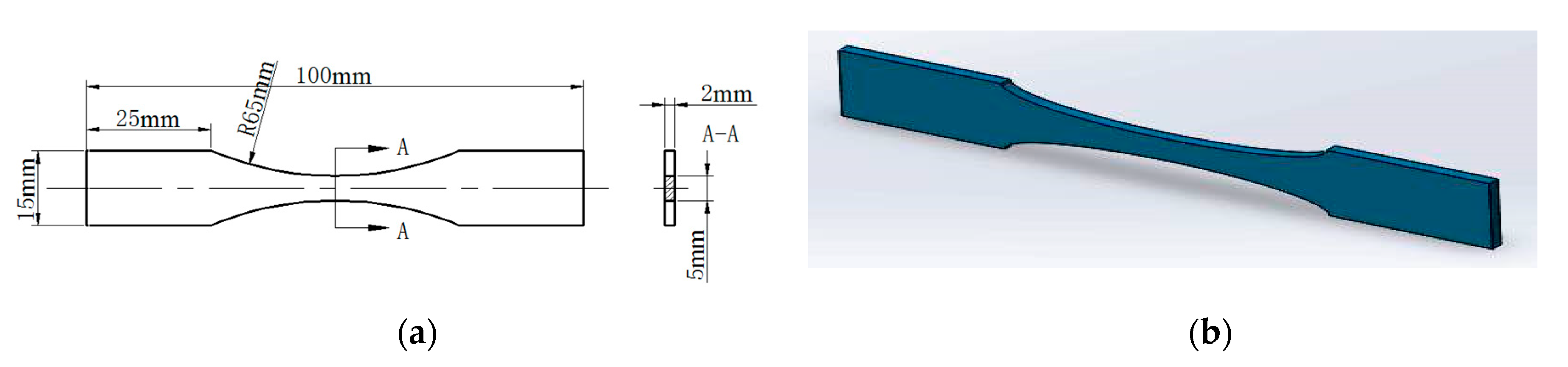
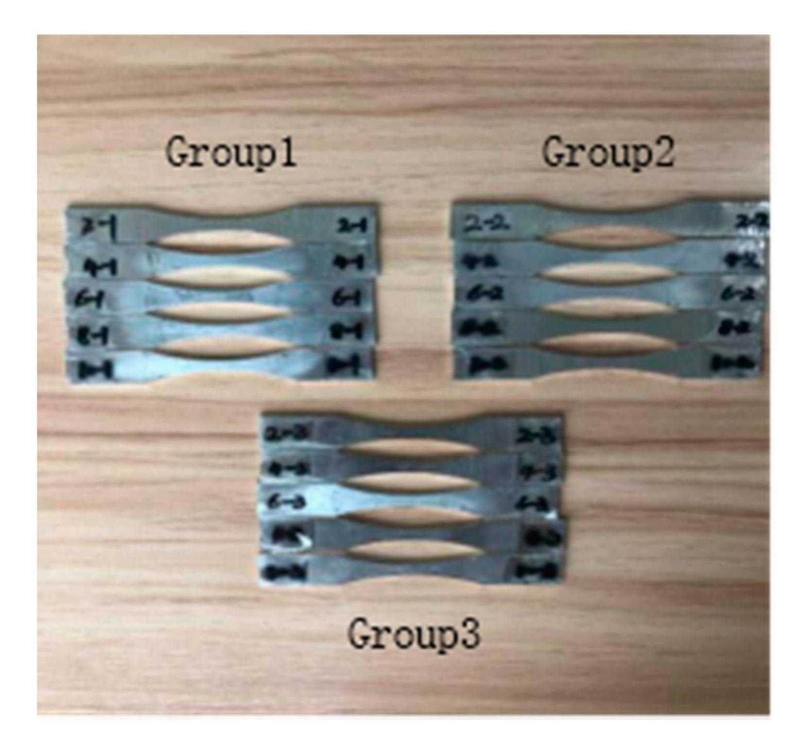
2.1. Material and Specimen Preparation
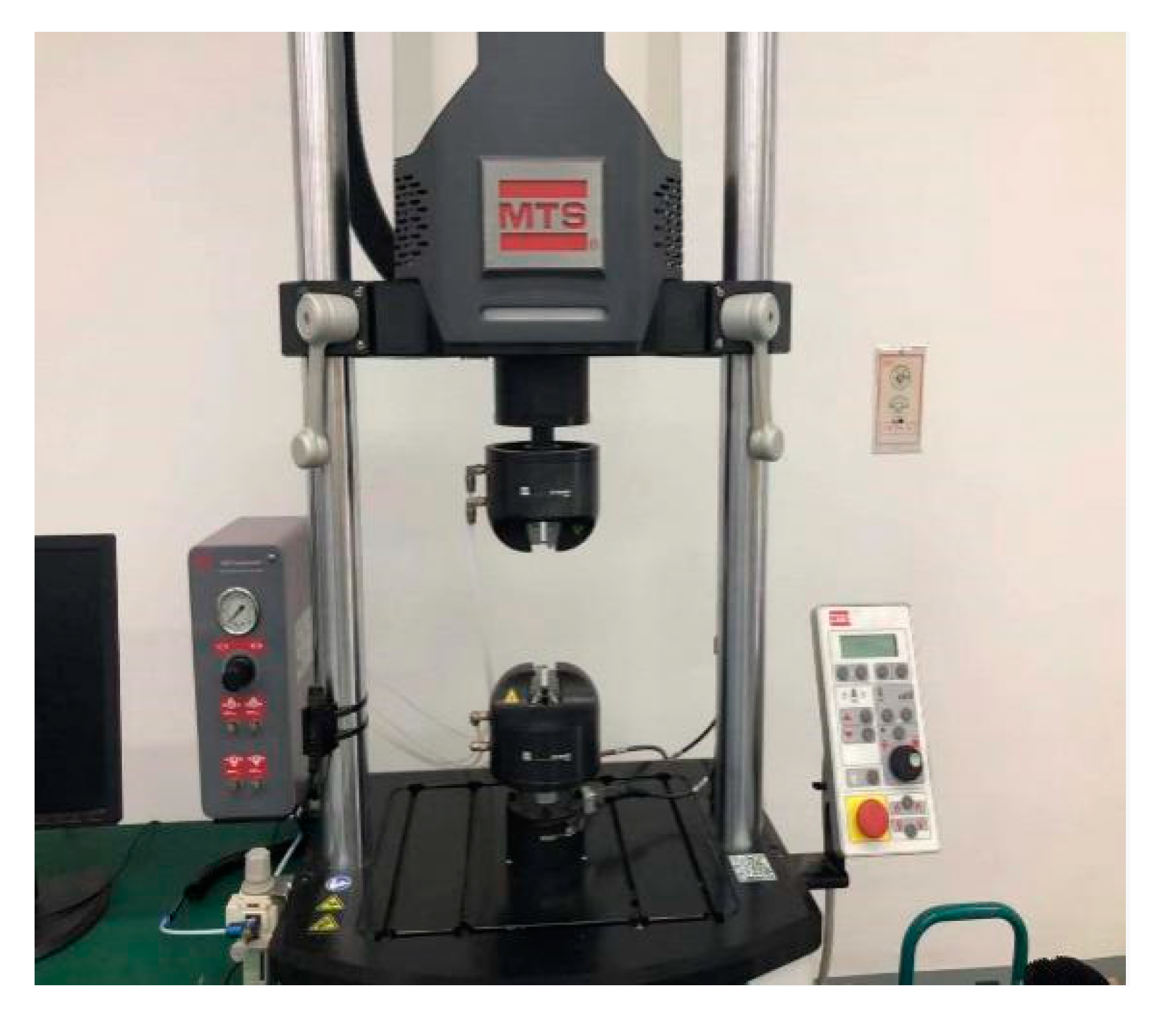
2.2. Fatigue Test Procedures
3. Acquisition and Analysis of Defect Characteristics Information
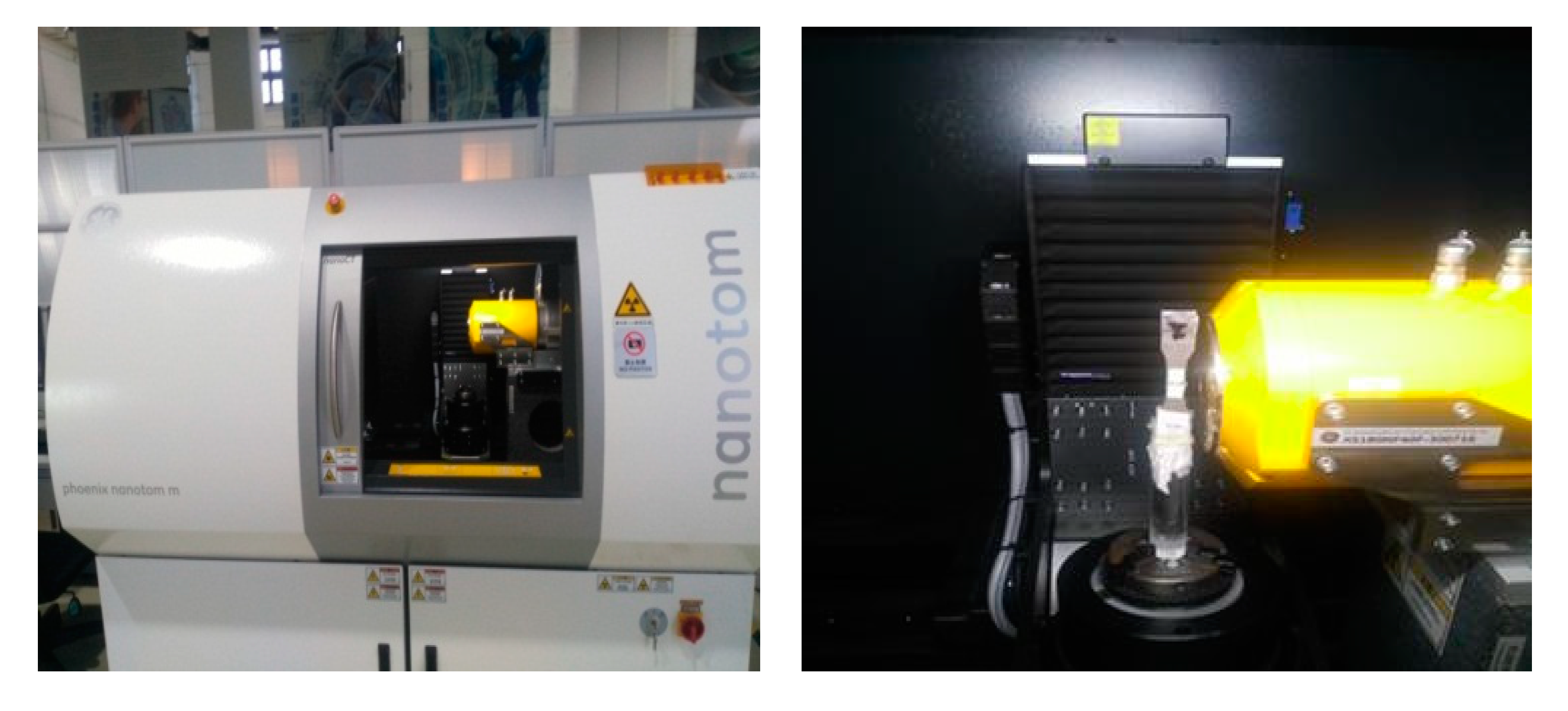
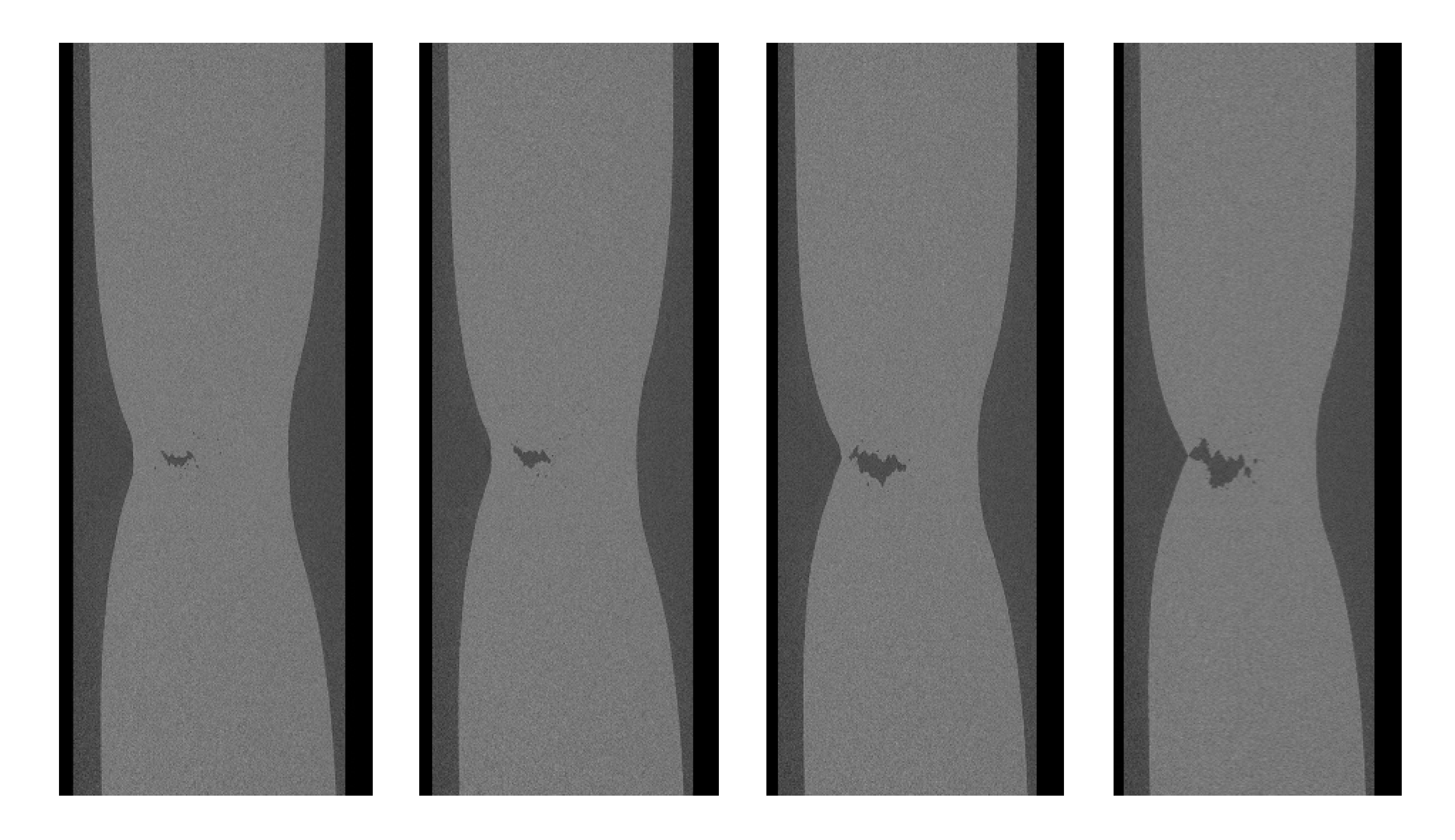
3.1. Acquisition of Defect by X-ray Micro-Computed Tomography (MCT)
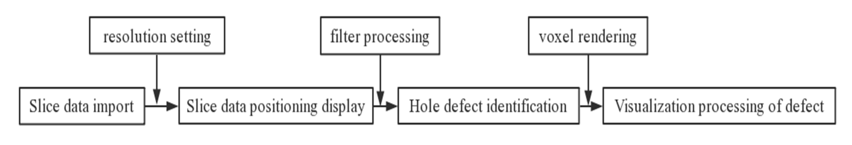
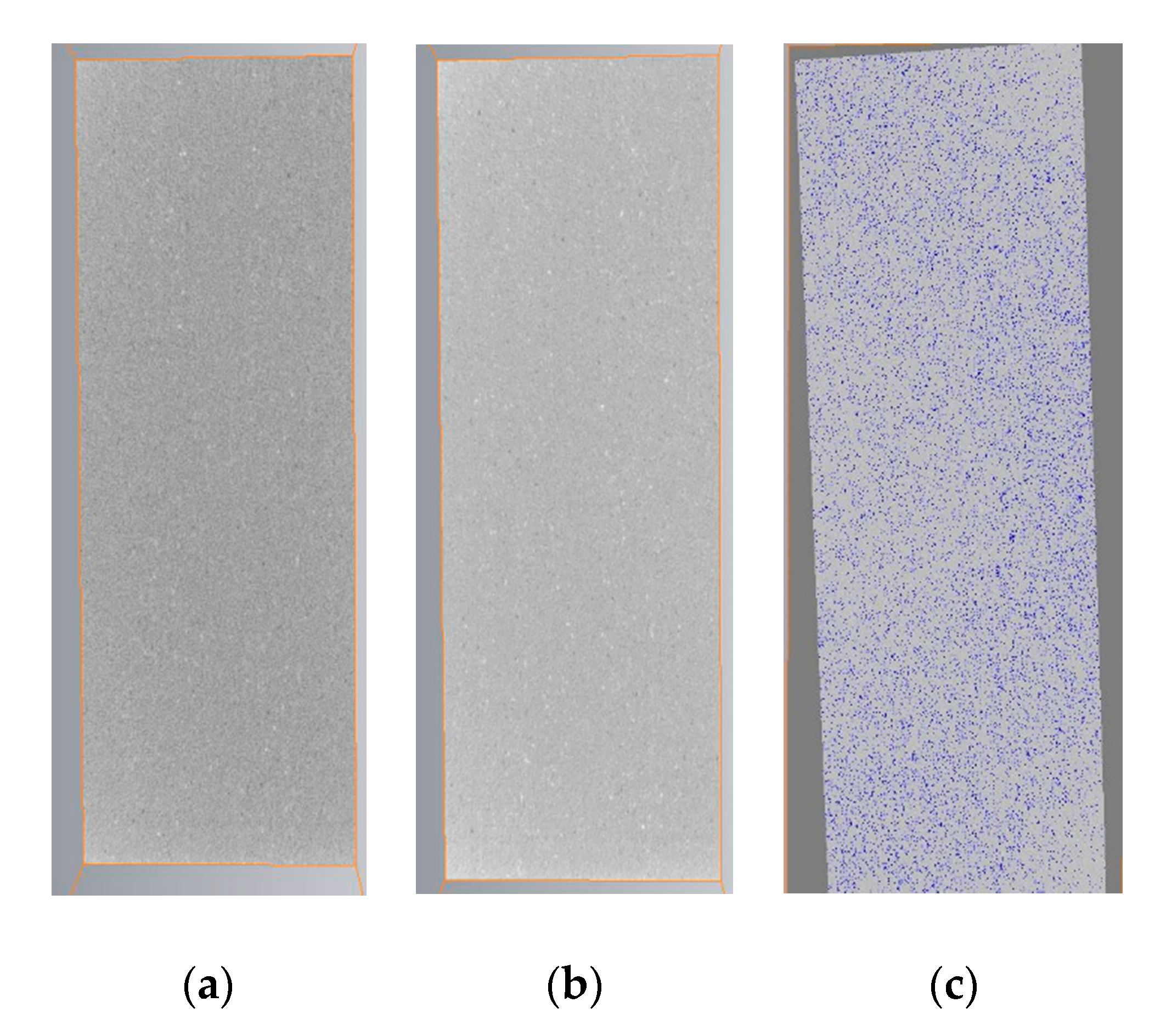
3.2. Visualization Processing of Defects Based on AVIZO
3.3. Extraction and Analysis of Defect Characteristic Information
4. Damage Model
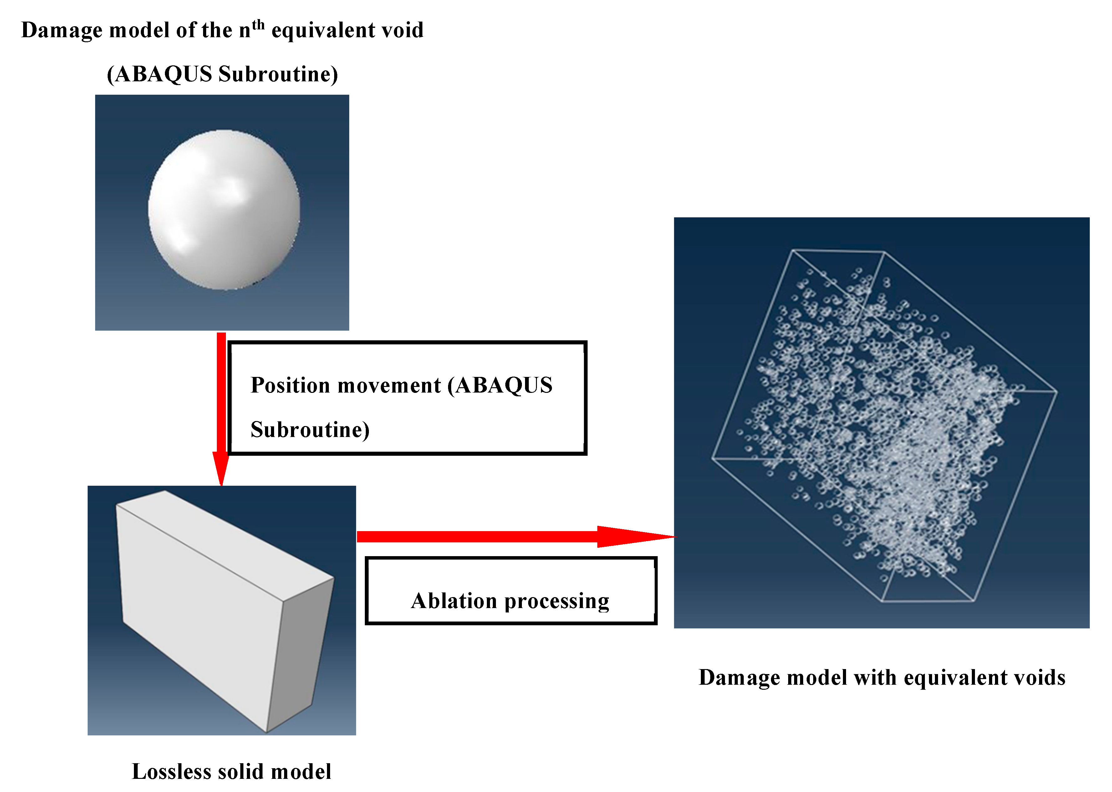
4.1. Establishment of an Equivalent Damage Model
4.2. Fatigue Model Analysis and Validation
5. Fatigue Life Prediction
6. Conclusions
- (1)
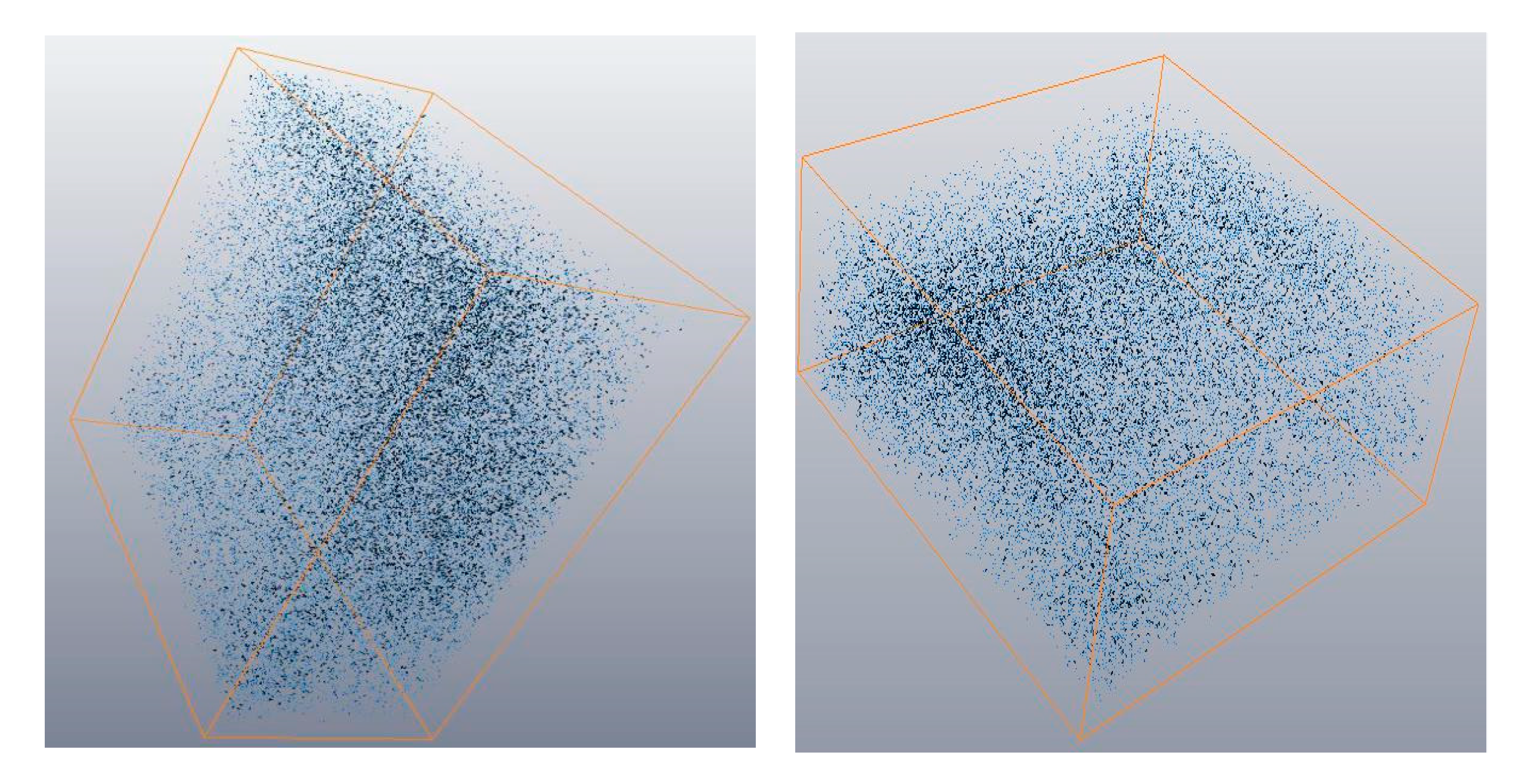
- The proposed method of defect classification was effective to realize the three-dimensional reconstruction of the mesoscopic defects based on the mesoscopic defect data obtained by CT scanning technology.
- (2)
- A new multiscale damage evolution model for fatigue damage accumulation had been developed, which built a bridge to describe the continuous average damage evolution process for metal fatigue components and structures in mesoscopic scale by macro damage variables for understanding metal fatigue failure mechanisms.
- (3)
- The fatigue life was predicted with the damage data measured by nondestructive testing technology (CT scanning technology, etc.) based on the effectiveness of the multiscale damage evolution model.
Author Contributions
Funding
Conflicts of Interest
References
- Kaynak, C.; Ankara, A.; Baker, T.J. Effects of short cracks on fatigue life calculations. Int. J. Fatigue 1996, 18, 25–31. [Google Scholar] [CrossRef]
- Lillbacka, R.; Johnson, E.; Ekh, M. A model for short crack propagation in polycrystalline materials. Eng. Fract. Mech. 2006, 73, 223–232. [Google Scholar] [CrossRef]
- Cheung, M.S.; Li, W.C. Probabilistic fatigue and fracture analyses of steel bridges. Struct. Saf. 2003, 23, 245–262. [Google Scholar] [CrossRef]
- Kachanov, L.M. Time of the rupture process under creep condition. TVZ Akad. Nauk. Ssr Otd. Tech. Nauk. 1958, 8, 26–31. [Google Scholar]
- Pathan, A.K.; Bond, J.; Gaskin, R.E. Sample preparation for scanning electron microscopy of plant surfaces—Horses for courses. Micron 2008, 39, 1049–1061. [Google Scholar] [CrossRef]
- Risitano, A.; Risitano, G. Cumulative damage evaluation of steel using infrared thermography. Appl. Fract. Mech. 2010, 54, 82–90. [Google Scholar] [CrossRef]
- Fan, J.L.; Guo, X.L.; Wu, C.W.; Zhao, Y. Research on fatigue behavior evaluation and fatigue fracture mechanisms of cruciform welded joints. Mater. Sci. Eng. 2011, A528, 8417–8427. [Google Scholar] [CrossRef]
- Fan, J.L.; Guo, X.L.; Wu, C.W. A new application of the infrared thermography for fatigue evaluation and damage assessment. Int. J. Fatigue 2012, 44, 1–7. [Google Scholar] [CrossRef]
- Belaadi, A.; Bezazi, A.; Bourchak, M.; Scarpa, F. Tensile static and fatigue behaviour of sisal fibres. Mater. Des. 2013, 46, 76–83. [Google Scholar] [CrossRef]
- Zhou, Y.F.; Jerrams, S.; Chen, L. Multi-axial fatigue in magnetorheological elastomers using bubble inflation. Mater. Des. 2013, 50, 68–71. [Google Scholar] [CrossRef]
- Azadi, M.; Farrahi, G.H.; Winter, G.; Eichlseder, W. Fatigue lifetime of AZ91 magnesium alloy subjected to cyclic thermal and mechanical loadings. Mater. Des. 2014, 53, 639–644. [Google Scholar] [CrossRef]
- Moreno-Navarro, F.; Rubio-Gámez, M.C. Mean damage parameter for the characterization of fatigue cracking behavior in bituminous mixes. Mater. Des. 2014, 54, 748–754. [Google Scholar] [CrossRef]
- Li, D.Z.; Han, L.; Thornton, M.; Shergold, M.; Williams, G. The influence of fatigue on the stiffness and remaining static strength of self-piercing riveted aluminium joints. Mater. Des. 2014, 54, 301–314. [Google Scholar] [CrossRef]
- Shiri, S.; Pourgol-Mohammad, M.; Yazdani, M. Probabilistic Assessment of Fatigue Life in Fiber Reinforced Composites. In Proceedings of the ASME 2014 International Mechanical Engineering Congress and Exposition, Montreal, QC, Canada, 10–14 November 2014; p. V014T08A018. [Google Scholar]
- Shiri, S.; Pourgol-Mohammad, M.; Yazdani, M. Effect of strength dispersion on fatigue life prediction of composites under two-stage loading. Mater. Des. 2015, 65, 1189–1195. [Google Scholar] [CrossRef]
- Shiri, S.; Yazdani, M.; Pourgol-Mohammad, M. A fatigue damage accumulation model based on stiffness degradation of composite materials. Mater. Des. 2015, 88, 1290–1295. [Google Scholar] [CrossRef]
- Miner, M.A. Cumulative damage in fatigue. J. Appl. Mech. 1945, 67, 159–164. [Google Scholar]
- Marco, S.M.; Starkey, W.L. A concept of fatigue damage. Trans. ASME 1954, 76, 627–632. [Google Scholar]
- Henry, D.L. A theory of fatigue damage accumulation in steel. Trans. ASME 1955, 77, 913–918. [Google Scholar]
- Gatts, R.R. Application of a cumulative damage concept to fatigue. J. Basic Eng. Trans. ASME 1961, 83, 529–540. [Google Scholar] [CrossRef]
- Manson, S.S.; Freche, J.C.; Ensign, C.R. Application of a Double Linear Damage Rule to Cumulative Fatigue; NASA TN D-3839; NASA: Washington, DC, USA, 1967.
- Chaboche, J.L.; Lesne, P.M. A non-linear continuous fatigue damage model. Fatigue Fract. Eng. Mater. Struct. 1988, 11, 1–17. [Google Scholar] [CrossRef]
- Manson, S.S.; Halford, G.R. Practical implementation of the double linear damage rule and damage curve approach for treating cumulative fatigue damage. Int. J. Fract. 1981, 17, 169–192. [Google Scholar] [CrossRef]
- Franke, L.; Dierkes, G. A non-linear fatigue damage rule with an exponent based on a crack growth boundary condition. Int. J. Fatigue 1999, 21, 761–767. [Google Scholar] [CrossRef]
- Miller, K.J.; Mohanmed, H.J.; DelosRios, E.R. The Behaviour of Short Fatigue Cracks; Mechanical Engineering Publications: London, UK, 1986. [Google Scholar]
- Angelova, D.; Akid, R. A note on modelling short fatigue crack behaviour. Fatigue Fract. Eng. Mater. Struct. 1998, 21, 771–779. [Google Scholar] [CrossRef]
- Polák, J.; Liškutíne, P. Nucleation and short crack growth in fatigued polycrystalline copper. Fatigue Fract. Eng. Mater. Struct. 1990, 13, 119–133. [Google Scholar] [CrossRef]
- McClintock, F.A. A criterion for ductile fracture by the growth of holes. J. Appl. Mech. Trans. Asme 1968, 35, 363–371. [Google Scholar] [CrossRef]
- Rice, J.R.; Tracey, D.M. On the ductile enlargement of voids in triaxial stress fifields. J. Mech. Phys. Solids 1969, 17, 201–217. [Google Scholar] [CrossRef]
- McDowell, D.L.; Gall, K.; Horstemeyer, M.F.; Fan, J. Microstructure-Based fatigue modeling of cast a356-t6 alloy. Eng. Fract. Mech. 2003, 70, 49–80. [Google Scholar] [CrossRef]
- Leuders, S.; Thöne, M. On the mechanical behaviour of titanium alloy TiAl6V4 manufactured byselective laser melting: Fatigue resistance and crack growth performance. Int. J. Fatigue 2013, 48, 300–307. [Google Scholar] [CrossRef]
- Hu, Y.N.; Wu, S.C.; Song, Z.; Fu, Y.N.; Yuan, Q.X.; Zhang, L.L. Effect of microstructural features on the failure behavior of hybrid laser welded AA7020. Fatigue Fract. Eng. Mater. 2018, 41, 2010–2023. [Google Scholar] [CrossRef]
- Desmorat, R.; Tertre, A.D.; Gaborit, P. Multiaxial haigh diagrams from incremental two scale damage analysis. AerospaceLab 2015, 1–15. [Google Scholar]
- Wan, H.L.; Wang, Q.; Chenxue, J.; Zhang, Z. Multi-Scale damage mechanics method for fatigue life prediction of additive manufacture structures of Ti-6Al-4V. Mater. Sci. Eng. A 2016, 669, 269–278. [Google Scholar] [CrossRef]
- Lemaitre, J.; Chaboche, J.L. Mechanics of Solid Materials; Cambridge University Press: Cambridge, UK, 1994. [Google Scholar]
- Lemaitre, J.; Desmorat, R. Engineering Damage Mechanics: Ductile, Creep, Fatigue and Brittle Failures; Springer Science & Business Media: Cachan, France, 2005. [Google Scholar]


| Chemical Composition | Cu | Si | Fe | Mn | Mg | Zn | Cr | Ti | Other | AL |
|---|---|---|---|---|---|---|---|---|---|---|
| Ratio | 25% | 60% | 70% | 15% | 85% | 25% | 16% | 15% | 15% | margin |
| Load Sequence (×104) | Stage | 2 | 4 | 6 | 8 | 10 |
|---|---|---|---|---|---|---|
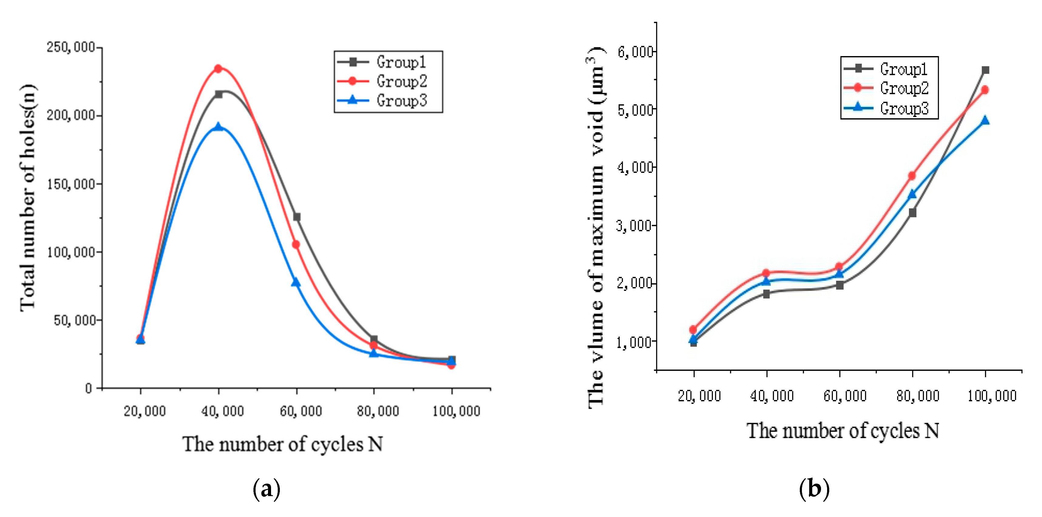
| Total number of voids (n) | Group1 | 35,106 | 215,398 | 125,703 | 35,684 | 20,982 |
| Group2 | 36,061 | 233,821 | 104,895 | 30,569 | 16,456 | |
| Group3 | 34,854 | 190,636 | 76,695 | 24,534 | 18,672 | |
| The volume of maximum void (μm3) | Group1 | 972 | 1810 | 1970 | 3210 | 5671 |
| Group2 | 1190 | 2161 | 2275 | 3841 | 5319 | |
| Group3 | 1021 | 2013 | 2144 | 3511 | 4782 | |
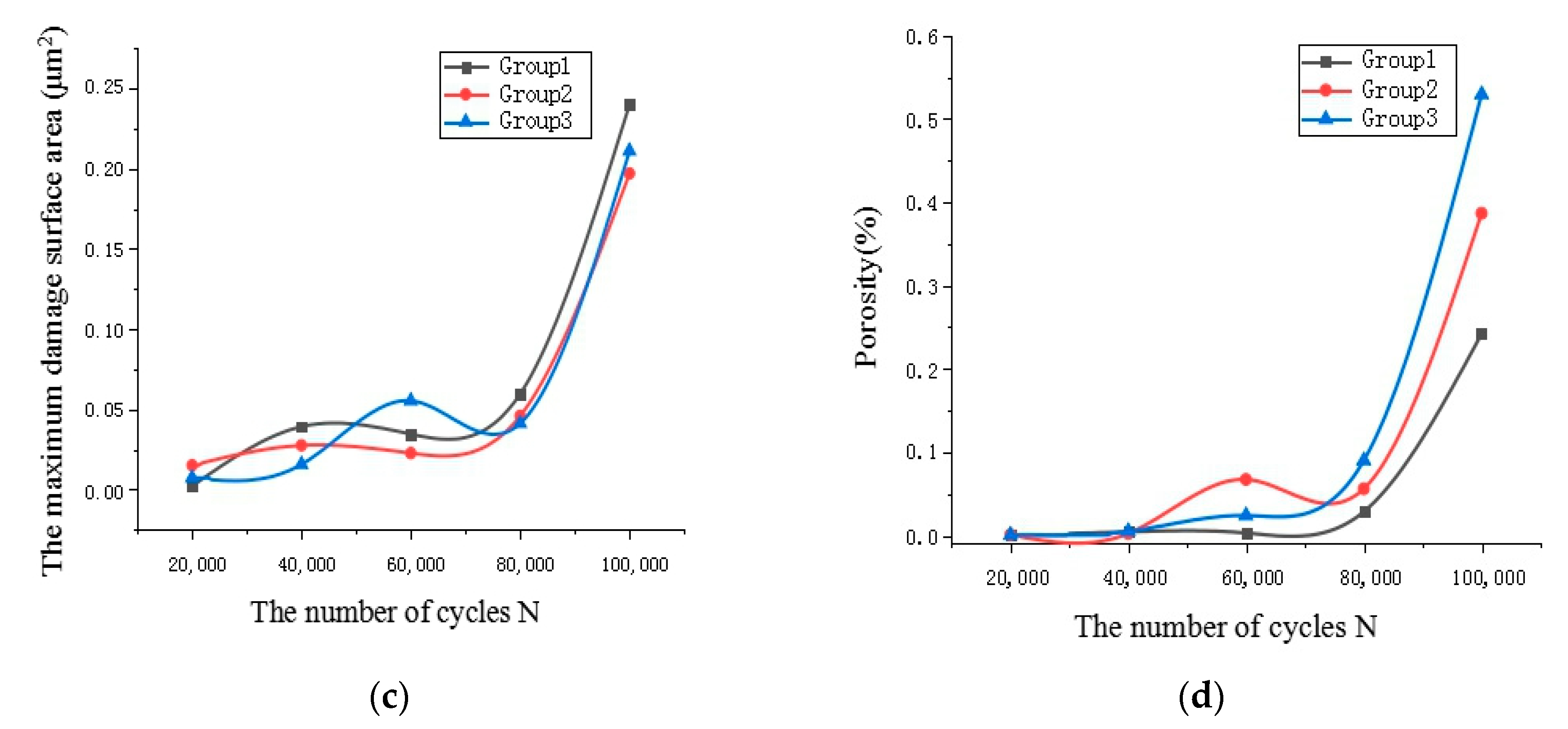
| Maximum damage surface area (μm2) | Group1 | 0.0022 | 0.0392 | 0.0345 | 0.0596 | 0.24 |
| Group2 | 0.0151 | 0.0275 | 0.0226 | 0.0459 | 0.197 | |
| Group3 | 0.0073 | 0.0157 | 0.0553 | 0.0412 | 0.211 | |
| Porosity (%) | Group1 | 0.0004 | 0.0046 | 0.0031 | 0.0287 | 0.2421 |
| Group2 | 0.0009 | 0.0025 | 0.0673 | 0.0562 | 0.3866 | |
| Group3 | 0.0006 | 0.0051 | 0.0242 | 0.0901 | 0.5293 |
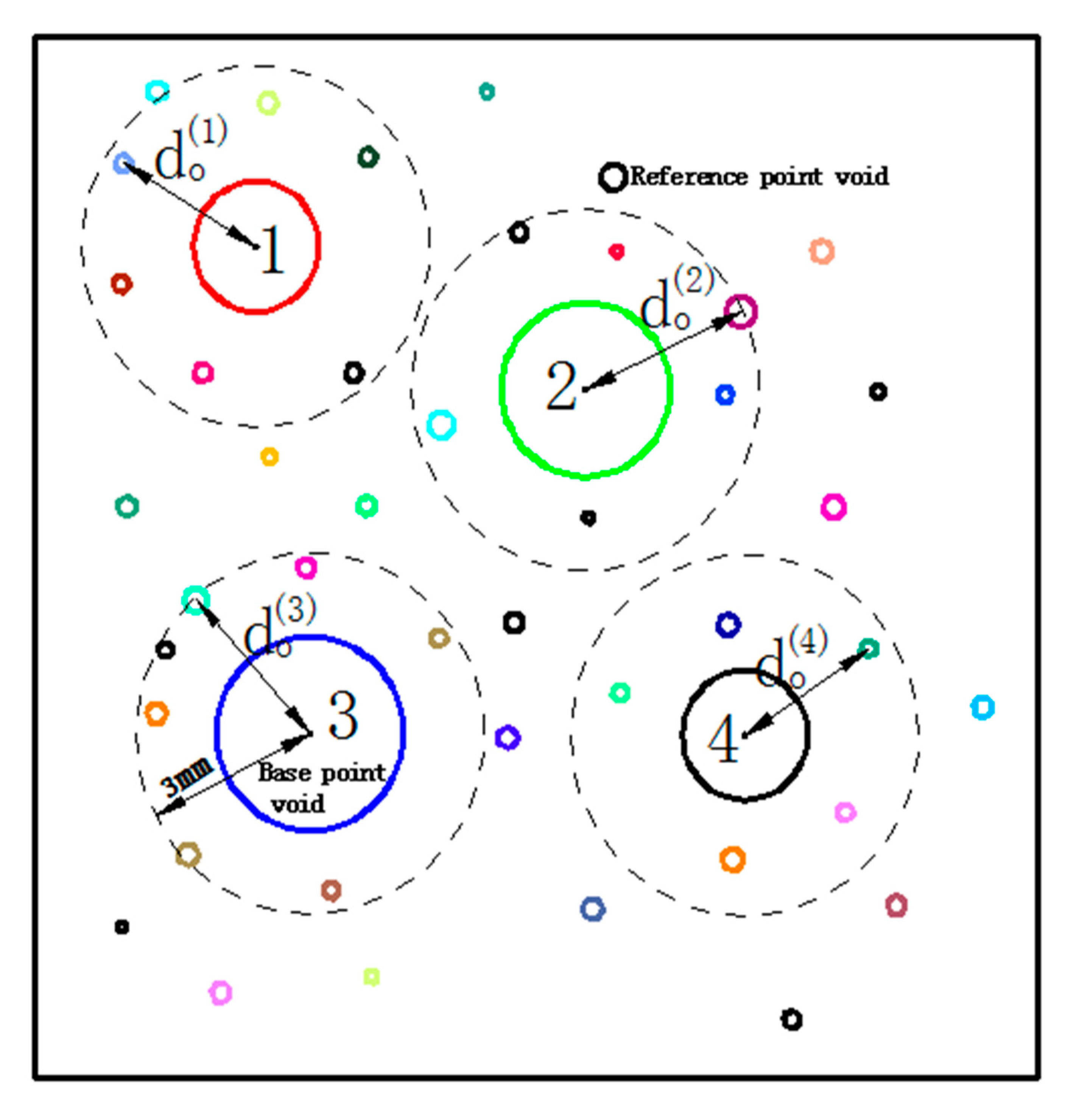
| Reference Point (n) | 1 | 2 | 3 | 4 | n | |
|---|---|---|---|---|---|---|
| 1 | 0 | 3.6457 | 5.1247 | 4.2487 | 3.8546 | |
| 2 | 3.6457 | 0 | 4.2136 | 4.8712 | 5.0147 | |
| 3 | 5.1247 | 4.2136 | 0 | 3.0014 | 3.2387 | |
| 4 | 4.2478 | 4.8712 | 3.0014 | 0 | 3.5601 | |
| n | 3.8546 | 5.0147 | 3.2387 | 3.5601 | 0 |
| load Sequence (×104) | Stage Group | 2 | 4 | 6 | 8 | 10 |
|---|---|---|---|---|---|---|
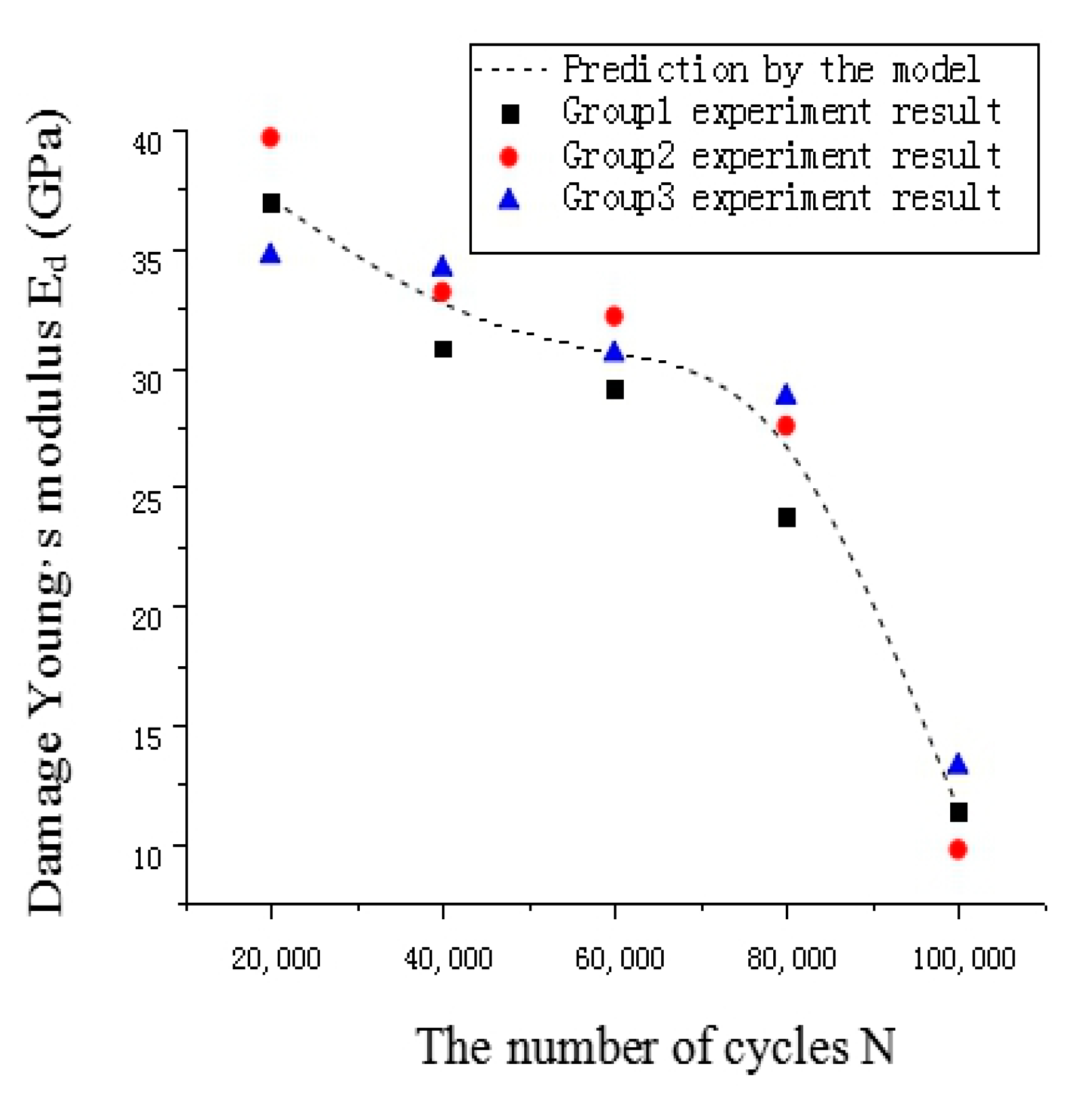
| Damage Young’s modulus Edt (GPa) | Group1 | 36.581 | 31.816 | 29.109 | 24.169 | 11.356 |
| Group2 | 39.647 | 33.169 | 32.147 | 27.549 | 9.365 | |
| Group3 | 34.946 | 34.149 | 30.564 | 28.764 | 13.248 |
© 2019 by the authors. Licensee MDPI, Basel, Switzerland. This article is an open access article distributed under the terms and conditions of the Creative Commons Attribution (CC BY) license (http://creativecommons.org/licenses/by/4.0/).
Share and Cite
Bao, Y.; Yang, Y.; Chen, H.; Li, Y.; Shen, J.; Yang, S. Multiscale Damage Evolution Analysis of Aluminum Alloy Based on Defect Visualization. Appl. Sci. 2019, 9, 5251. https://doi.org/10.3390/app9235251
Bao Y, Yang Y, Chen H, Li Y, Shen J, Yang S. Multiscale Damage Evolution Analysis of Aluminum Alloy Based on Defect Visualization. Applied Sciences. 2019; 9(23):5251. https://doi.org/10.3390/app9235251
Chicago/Turabian StyleBao, Yuquan, Yali Yang, Hao Chen, Yongfang Li, Jie Shen, and Shuwei Yang. 2019. "Multiscale Damage Evolution Analysis of Aluminum Alloy Based on Defect Visualization" Applied Sciences 9, no. 23: 5251. https://doi.org/10.3390/app9235251
APA StyleBao, Y., Yang, Y., Chen, H., Li, Y., Shen, J., & Yang, S. (2019). Multiscale Damage Evolution Analysis of Aluminum Alloy Based on Defect Visualization. Applied Sciences, 9(23), 5251. https://doi.org/10.3390/app9235251