Currency Crises Prediction Using Deep Neural Decision Trees

Featured Application

The superiority of a novel computational technique (deep neural decision trees) for prediction of currency crises over other methodologies and the construction of new crisis prediction models more precise than existing ones.

Abstract

Currency crises are major events in the international monetary system. They affect the monetary policy of countries and are associated with risks of vulnerability for open economies. Much research has been carried out on the behavior of these events, and models have been developed to predict falls in the value of currencies. However, the limitations of existing models mean further research is required in this area, since the models are still of limited accuracy and have only been developed for emerging countries. This article presents an innovative global model for predicting currency crises. The analysis is geographically differentiated for regions, considering both emerging and developed countries and can accurately estimate future scenarios for currency crises at the global level. It uses a sample of 162 countries making it possible to account for the regional heterogeneity of the warning indicators. The method used was deep neural decision trees (DNDTs), a technique based on decision trees implemented by deep learning neural networks, which was compared with other methodologies widely applied in prediction. Our model has significant potential for the adaptation of macroeconomic policy to the risks derived from falls in the value of currencies, providing tools that help ensure financial stability at the global level.

1. Introduction

Currency crises can have a catastrophic impact on the real economy in a short space of time. In general, they occur when there is a sudden devaluation in a currency, often resulting in a speculative attack on the international currency market. Currency crises can also occur as a result of high balance of payments deficits or when governments are unable to restore the value of their currency after a fall in its price in the markets.

One of the first currency crises occurred in 1992 when many European countries faced a crisis as part of the Exchange Rate Mechanism (ERM). Another episode was the currency crisis suffered by the Mexican peso in December 1994. This crisis began with an abrupt decision by the Mexican government to devalue its currency, causing a crash in the peso days later and an economic crisis that resulted in a sharp drop in GDP. However, the biggest event has been the Asian Financial Crisis in 1997. The crisis began with the sharp devaluation of the Thai baht and was the first to show the effect of contagion on other countries. However, the event was about more than just speculation on the Thai currency and saw the collapse of Asian stock markets. The financial crisis that began with the devaluation of the Thai baht exchange rate resulted in a sharp increase in interest rates and the collapse of many companies, as well as an increase in the cost of credit and a general fall in GDP in the region [1]. This resulted in foreign and national investors pulling out investment. Not only did this crisis affect Asian countries, but it also had a negative impact on other emerging economies, especially in Latin America, showing that currency crises are not limited to a specific economy. Globalization can increase the economic difficulties of societies and affect the structure of national economies after the real economy has suffered a damaging impact [2]. 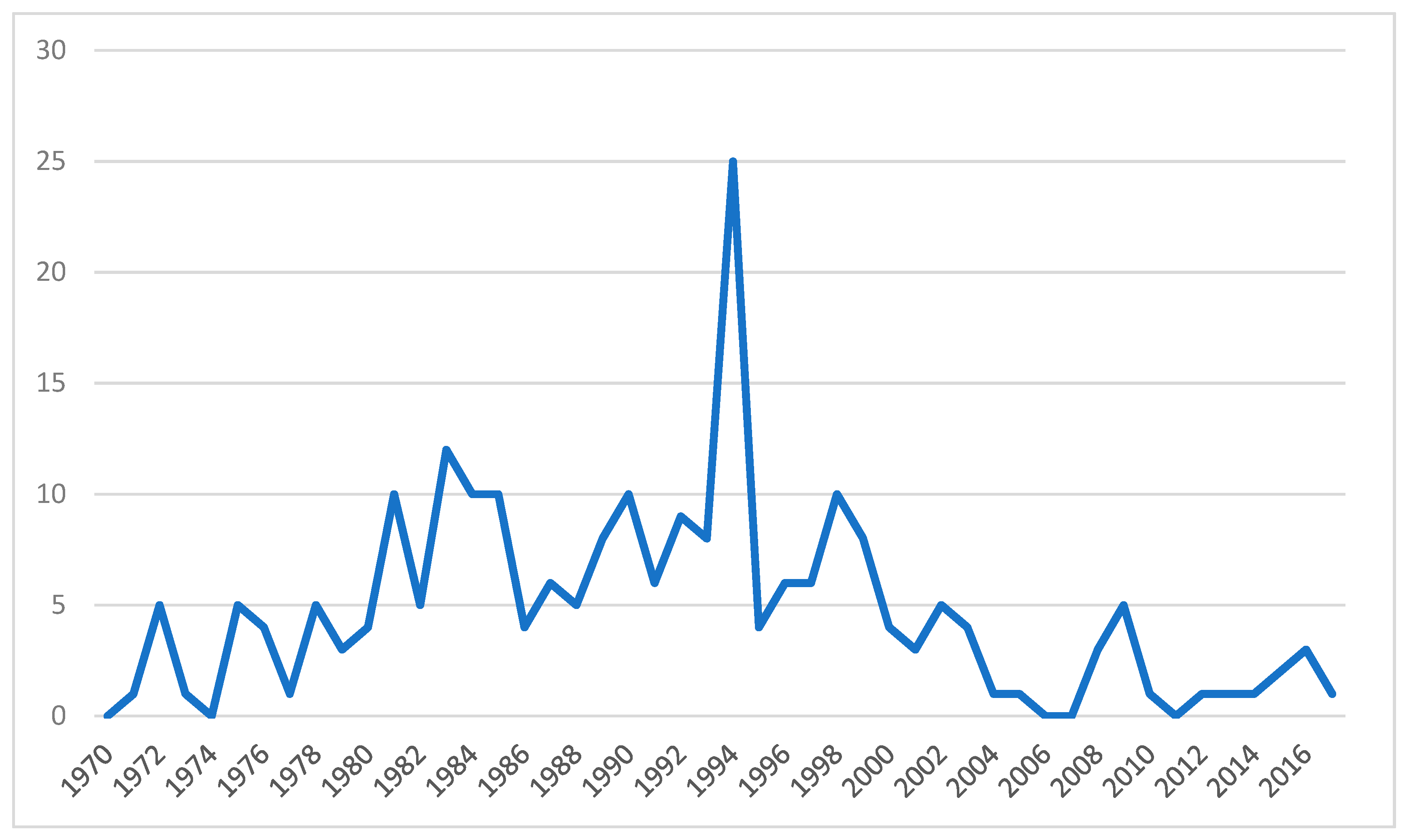Figure 1 shows the number of currency crises per year at the international level.

On the other hand, it is interesting to influence the economic consequences that currency crises can cause. Reference [3] demonstrated that a currency crisis makes it difficult to design an optimal monetary policy, making the setting of the interest rate a dilemma; since, if it increases, it makes it difficult to lend money to companies, and, if it decreases, it devalues the debt denominated in foreign currency. They concluded that the best decision is to reduce the interest rate, thanks to the continuous international financial development and the increase in credit flows. Following this argument, some works indicated that currency crises deteriorate the balance sheets of companies based on the fact that, if prices are rigid, a depreciation of the currency leads to an increase in the obligations of payment of the debt in the foreign currency of companies, causing a fall in their profits [4,5]. This reduces the borrowing capacity of companies and, therefore, investment and production in an economy with credit limitations which, in turn, reduces the demand for the national currency and leads to depreciation. Other authors presented a general equilibrium model of currency crises and how they are driven by credit restrictions and rigidity of nominal prices [6,7,8]. They showed that an increase in the interest rate to support the currency in crisis may not be effective, but that relaxation of short-term loan facilities can make this policy effective by mitigating the increase in interest rates for companies [9]. In addition to interest rate policy being an instrument to end a currency crisis, intervention in the foreign exchange market is also a measure to stabilize inflation and production as a result of this type of crisis. They demonstrated how intervention in the foreign exchange market improves the situation of the economy, regardless of the exchange rate regime chosen by the country. It can achieve great results if the economy encounters imperfect capital mobility/asset substitutability movements, producing the same result as discretionary monetary policy and without jeopardizing the inflation target [9,10,11].

To avoid future crises, researchers have tried to identify common factors underlying exchange rate instability and develop predictive models. However, despite impressive results for in-sample, the existing early warning models encounter difficulties when it comes to predicting crises outside it [12,13,14].

In recent years, there has been considerable research on currency crises, mainly on the application of computational techniques for emerging economies. Statistical methods have also been used, albeit with limited success. For example, Reference [12] applied extreme value theory, obtaining an accuracy of 44%. Reference [15] developed a discrete choice early warning system considering the persistence of the phenomenon of the crisis. Their logistic regression system used a maximum likelihood estimation method both country-by-country and in a panel framework. The model obtained predictive capacity that significantly improved the existing static models, both inside and outside the sample (89.8% and 90.2%, respectively).

Reference [1] used computational combinations with support vector machine (SVM), logistic regression, and logical analysis of data tree (LADTree), based on the k-nearest neighbor. The results showed that the computational classifiers were more accurate than the traditional statistical methods, obtaining a level above 90%. Reference [2] individually used SVM for the currency crisis in Argentina, obtaining a high level of robustness. Similarly, Reference [13] studied currency crises in developed countries using the classification and regression tree methodology (CART) and random forest (RF). Their findings determined that significant factors included high short-term domestic interest rates and overvalued exchange rates. Reference [16] compared logistic regression, neural networks (NNs), and decision trees (DTs) to predict the currency crisis in Turkey, with NNs achieving the highest level of accuracy. Also for Turkey, Reference [17] used logistic regression to analyze the determinants of the currency and banking crisis. The study found that currency crises are caused by an excessive fiscal deficit, short-term increases in external debt, overvaluation of the Turkish lira, and adverse external shocks, confirming the results obtained by other studies based on the experiences of emerging countries [18,19].

This study attempted to build more accurate models for predicting currency crises. To do so, we developed models for four regions of the world (i.e., Latin America, Asia, Africa, and the Middle East and Europe) together with a global model for all world regions. This study thus sought to address a gap in the literature, which requires broader models that can provide powerful and homogeneous empirical tools for public institutions in different countries. It did this using the deep neural decision trees (DNDTs) methodology, developed in Reference [20], which allows for solutions to forecasting problems involving data outside of a sample, also one of the least resolved aspects in the existing literature. We compared this novel method in terms of accuracy with other popular methodologies used in time-series prediction such as regression logistic, neural networks, support vector machines, and AdaBoost.

The rest of this article is organized as follows: Section 2 describes the DNDTs algorithm, and Section 3 summarizes the data and variables used as possible predictors. The results and their comparison with the existing literature are provided in Section 4. Finally, Section 5 summarizes the main conclusions.

2. Methodology

As already stated above, the DNDT algorithm was applied to solve the research question raised, but we have also used different methods in the construction of the currency crisis prediction model. The use of different methods aimed to achieve a robust model which is contrasted not only through a classification technique but also by applying all those that have shown success in the previous literature [1,2,12,13,14]. Specifically, logistic regression, artificial neural networks, support vector machines, and AdaBoost were used. A synthesis of the methodological aspects of each of these classification techniques appears below.

2.1. Logistic Regression

The logistic regression model (Logit) is a non-linear classification model, although it contains a linear combination of parameters and observations of the explanatory variables [21]. The logistic function is bounded between 0 and 1, thus providing the probability that an element is in one of the two established groups. From a dichotomous event, the Logit model predicts the probability that the event will or will not take place. If the probability estimate is greater than 0.5, then the prediction is that it does belong to that group, otherwise it would assume that it belongs to the other group considered. To estimate the model, we started from the quotient between the probability that an event will occur and the probability that it will not occur. The probability of an event occurring is determined by Expression (1).

$$P\left(Y_i=\frac{1}{x_i}\right)=\frac{e^{\left({\beta }_0+{\beta }_1+X_1+\dots +{\beta }_k{X}_k\right)}}{1+e^{\left({\beta }_0+{\beta }_1+X_1+\dots +{\beta }_k{X}_k\right)}}=\frac{1}{1+e^{-\left({\beta }_0+{\beta }_1+X_1+\dots +{\beta }_k{X}_k\right)}}$$

(1)

where β₀ is the constant term of the model and β₁, …, β_k are the coefficients of the variables.

2.2. Support Vector Machines

Support vector machines (SVMs) have been shown to achieve good generalization performance over a wide variety of classification problems, where it is seen that SVM tends to minimize generalization errors, that is, classifier errors over new instances. In geometric terms, SVM can be seen as the attempt to find a surface (σ_i) that separates positive examples from negative ones by the widest possible margin [22,23,24].

The search that meets the minimum distance between it and an example of training is the maximum and is performed across all surfaces (σ₁, σ₂…) in the A-dimensional space that separates the positive examples from the negative in the training set (known as decision surfaces). To better understand the idea behind the SVM algorithm, we take the case in which the positive and negative examples are linearly separable; therefore, the decision surfaces are |A|-1-hyperplanes. For example, in the case of two dimensions, several lines can be taken as decision surfaces. In this circumstance, the SVM method chooses the middle element of the widest set of parallel lines, that is, from the set in which the maximum distance between two of its elements is the greatest. It should be noted that the best decision surface is determined only by a small set of training examples, called support vectors.

An important advantage of SVM is that it allows the construction of non-linear classifiers, that is, the algorithm represents non-linear training data in a high-dimensional space (called the characteristic space) and builds the hyperplane that has the maximum margin. In addition, due to the use of a kernel function to perform the mapping, it is possible to calculate the hyperplane without explicitly representing the feature space.

In the present work, the method of minimum sequential optimization (SMO) was used to train the SVM algorithm. In general, SMO divides a large number of quadratic programming (QP) problems that need to be solved in the SVM algorithm by a series of smaller QP problems.

2.3. Artificial Neural Networks (Multilayer Perceptron)

A multilayer perceptron (MLP) is a feedforward artificial neural network model of supervised learning which is composed of a layer of input units (sensors), another output layer, and a certain number of intermediate layers, called hidden layers, in so much that they have no connections with the outside. Each input sensor is connected to the units of the second layer and these in turn with those of the third layer, etc. The network aims to establish a correspondence between a set of input data and a set of desired outputs.

Reference [25] confirmed that learning in MLP is a special case of functional approximation, where there is no assumption about the model underlying the analyzed data. This process involves finding a function that correctly represents the learning patterns, in addition to carrying out a generalization process that allows to efficiently treat individuals not analyzed during said learning [26]. For this, we proceed to the adjustment of weights, W, from the information from the sample set, considering that both the architecture and the connections of the network are known, being the objective to obtain those weights that minimize the learning error. Given, then, a set of pairs of learning patterns {(x₁, y₁), (x₂, y₂) … (x_p, y_p)} and an error function ε (W, X, Y), the training process implies the search for the set of weights that minimizes the learning error E(W) [27], as expressed in Equation (2).

$$\underset{W}{min}E\left(W\right)=\underset{W}{min}{\displaystyle \sum }_{i=1}^p\epsilon (W,x_i,y_i)$$

(2)

2.4. AdaBoost

AdaBoost is a meta-algorithm learning machine that can be used in conjunction with many other types of learning algorithms to improve its performance. The output of the other learning algorithms of the “weak” classifiers is combined in a weighted sum representing the final output of the driven classifier. AdaBoost is adaptive in the sense that weak posterior classifiers are adjusted in favor of those cases poorly classified by previous classifiers. AdaBoost is sensitive to noisy data and outliers. In some problems, however, it may be less susceptible to problems than other learning algorithms [28].

While each learning algorithm tends to adapt to some types of problems better than others, and usually has many different parameters and configurations to adjust before achieving optimal performance in a data set, AdaBoost (with decision trees such as weak classifiers) is often referred to as the best classifier outside the sample. Unlike neural networks and SVMs, the AdaBoost training process selects only those characteristics known to improve the predictability of the model, reduce dimensionality, and, potentially, improve the execution time of functions as irrelevant that do not need to be calculated.

AdaBoost refers to a method of training a driven classifier [29]. A boost classifier is designed as follows:

$$F_T\left(x\right)={\displaystyle \sum }_{t=1}^T{f}_t\left(x\right)$$

(3)

where each f_t is a weak learner that takes an object x as input and returns a result of real value that indicates the class of the object. The weak classifier output signal identifies the predicted object class and the absolute value gives confidence in that classification. Similarly, the T of the layer classifier will be positive if the sample is believed to be in the positive and negative class in another way.

Each weak classifier produces an output, the hypothesis h(x_i), for each sample in the training set. In each iteration t, a weak learner is selected and assigned a coefficient α_t such that the training error sum E_t of the resultant t of the classifying pulse is minimized.

$$E_t={\displaystyle \sum }_{i}E\left[F_{t-1}\left(x_i\right)+{\alpha }_{t}h\left(x_i\right)\right]$$

(4)

where F_t−1 is the driven classifier that has been built up to the previous stage of the formation, E(F) is the error function, and f_t (x) = α_th(x) is the weak beginner being considered for the addition to the final classifier.

2.5. Deep Neural Decision Trees (DNDTs)

Deep neural decision trees are DT models executed by deep-learning NNs, where a configuration of DNDT weightings corresponds to a specific decision tree and is thus interpretable [20]. Nevertheless, as DNDT is performed by the NN, it has several different properties of conventional DTs: DNDTs can be implemented from the NN structure in software such as Python (Pytorch). All parameters are optimized simultaneously with stochastic gradient descent (SGD) instead of a complex greedy splitting procedure; this allows large-scale processing with mini-batch-based learning and can be connected to any larger NN model for end-to-end learning with backward propagation. Continuing with this explanation, conventional DTs learn through a greedy and recursive division of characteristics [30]. This may have benefits with respect to the selection of functions; however, this greedy search may become inefficient [31]. Some recent work explores alternative approaches to train decision trees that aim to achieve better performance, for example, with a latent variable structured prediction [31]. On the other hand, a DNDT is much simpler, but we can still find the best solutions compared to conventional DT inductors when looking for the structure and parameters of the tree with SGD. Finally, while conventional DT inductors only use binary divisions to simplify, DNDT can also work with arbitrary cardinality divisions which can sometimes generate more interpretable trees. The algorithm begins by implementing a soft binning function to calculate the error rate for each node, making it possible to make decisions divided into DNDTs [32]. In general, the input of a binning function is a real scalar x which generates an index of the containers to which x belongs. Assuming x is a continuous variable, group it into n + 1 intervals. This requires n cut-off points which are trainable variables in this context. The cut-off points are denoted as (β₁, β₂, …, β_n) and are strictly ascending such that β₁ < β₂ < … < β_n.

The activation function of the DNDT algorithm is implemented based on the NN defined in Equation (1).

π = fw,b,τ (x) = softmax((wx + b)/τ)

(5)

where w is a constant with value w = [1, 2, …, n + 1], τ > 0 is a temperature factor, and b is defined in Equation (6).

b = [0, −β₁, −β₁, −β₂, …, −β₁ − β₂ − … − β_n]

(6)

The NN defined in Equation (1) gives a coding of the binning function x. Additionally, if τ tends to 0 (often the most common case), the vector sampling is implemented using the Straight-Through (ST) Gumbel–Softmax method [33].

Given the binning function described above, the key idea is to build the DT using the Kronecker product. Assuming we have an input instance x ∈ R^D with D characteristics. Associating each characteristic x_d with its own NN f_d (x_d), we can determine all the final nodes of the DT, in line with Equation (7).

z = f₁(x₁) ⊗ f₂(x₂) ⊗ … ⊗ f_D(x_D)

(7)

where z is now also a vector that indicates the index of the leaf node reached by instance x. We assume that a linear classifier on each leaf z classifies the instances that reach it. The number of cut points per feature is the complexity parameter of the model. The cut-off point values are not limited, which means that some of them may be inactive. For example, they are smaller than the minimum x_d or greater than the maximum x_d.

With the method described so far, we can route the input instances to the leaf nodes and classify them. Therefore, training a decision tree becomes a matter of training the cut-off points of the container and the sheet sorters. Since all steps forward are differentiable, all parameters can be trained directly and simultaneously with SGD.

The DNDT scales well with the number of inputs due to the training of the mini-batches of the NN. However, the main drawback of the design is the use of the Kronecker product, which means it is not scalable in terms of the number of characteristics. In our current implementation, we avoided this problem by using broad datasets, training a forest with a random subspace [34]. This involved introducing multiple trees and training each with a subset with random characteristics. A better solution that does not require a forest of hard interpretability involves exploiting the dispersion of the binning function during the learning since the number of non-empty leaves grows much slower than the total.

2.6. Sensitivity Analysis

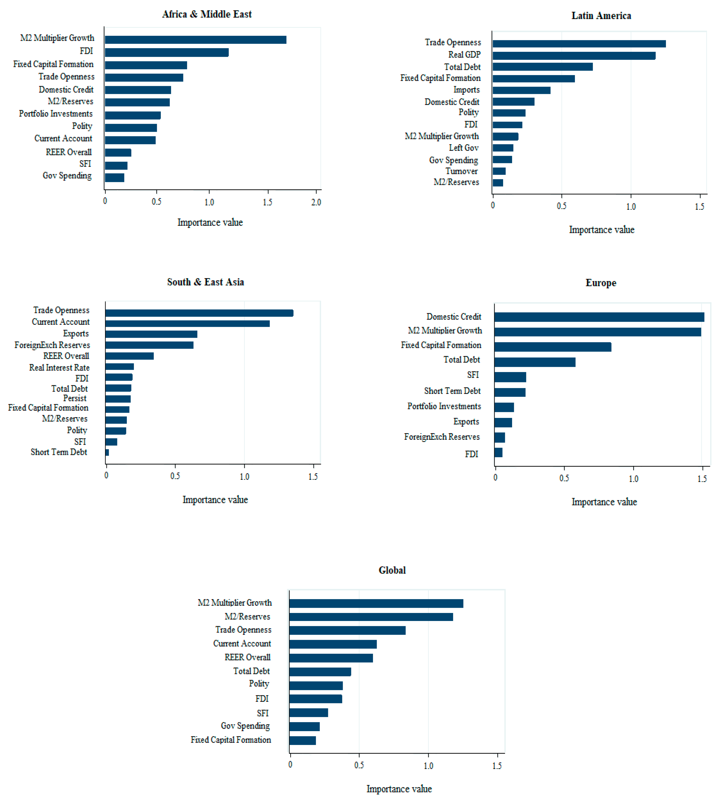
While DTs have a high explanatory capacity, when numerous exploratory variables are used, we need indicators to show the determined impact of these variables. Sensitivity analysis is used for this purpose, allowing the quantification of the relative significance of the independent variables related to the dependent variable [35]. The DT models used in this study build an appropriate measure of significance as shown in

Table A3. Variable significance values of variables for Currency Crisis.

Variables	Africa and Middle East	Latin America	South and East Asia	Europe	Global
Total Debt	0.000	0.726	0.183	0.586	0.439
Short Term Debt	0.000	0.000	0.024	0.225	0.000
Real Interest Rate	0.000	0.000	0.204	0.000	0.000
Foreign Exchange Reserves	0.000	0.000	0.634	0.079	0.000
Trade Openness	0.748	1.253	1.351	0.000	0.834
Imports	0.000	0.415	0.000	0.000	0.000
Exports	0.000	0.000	0.657	0.128	0.000
Current Account	0.483	0.000	1.181	0.000	0.624
Portfolio Investments	0.531	0.000	0.000	0.142	0.000
FDI	1.178	0.217	0.192	0.055	0.375
Real GDP	0.000	1.173	0.000	0.000	0.000
Real GDP Growth	0.000	0.000	0.000	0.000	0.000
Inflation	0.000	0.000	0.000	0.000	0.000
M2 Multiplier Growth	1.732	0.186	0.000	1.494	1.248
M2/Reserves	0.620	0.073	0.155	0.000	1.172
REER Overall	0.249	0.000	0.349	0.000	0.597
Government Spending	0.184	0.142	0.000	0.000	0.214
Fixed Capital Formation	0.785	0.593	0.172	0.843	0.187
Unemployment	0.000	0.000	0.000	0.000	0.000
Contagion	0.000	0.000	0.000	0.000	0.000
Soft Peg	0.000	0.004	0.000	0.000	0.000
Peg	0.000	0.000	0.000	0.000	0.000
Domestic Credit	0.627	0.301	0.000	1.518	0.000
Lending Interest Rate	0.000	0.000	0.000	0.000	0.000
Deposit Interest Rate	0.000	0.000	0.000	0.000	0.000
Polity	0.493	0.239	0.147	0.000	0.382
Durable	0.000	0.000	0.000	0.000	0.000
Persist	0.000	0.000	0.182	0.000	0.000
SFI	0.211	0.000	0.085	0.231	0.275
Left Government	0.000	0.151	0.000	0.000	0.000
Election	0.000	0.000	0.000	0.000	0.000
Turnover	0.000	0.096	0.000	0.000	0.000
Years	0.000	0.000	0.000	0.000	0.000
Economic Effectiveness	0.000	0.000	0.000	0.000	0.000

. The sensitivity analysis is also used to reduce the models to the most significant variables, eliminating or ignoring those of lesser significance. A variable is considered more significant than another if it increases the variance compared to the set of variables of the model. Each DT model generates significance scores for each independent variable. This is done using the Sobol method [36], which decomposes the variance of the total output V(Y) in line with the equations in Equation (8).

$$V\left(Y\right)={\displaystyle \sum }_i{V}_i+{\displaystyle \sum }_i{\displaystyle \sum }_{j>1}{V}_{ij}+\dots +V_{12\dots k}$$

(8)

where $V_i=V\left(E\left(Y|X_i\right)\right)$ and $V_{ij}=V\left(E\left(Y|X_i,X_j\right)\right)-V_i-V$.

The sensitivity indexes are determined by S_i = V_i/V and S_ij = V_ij/V, where S_ij indicates the effect of the interaction between two factors. The Sobol decomposition allows the estimation of a total sensitivity index ST_i which measures the sum of all the sensitivity effects involved in the independent variables.

2.7. Research Steps

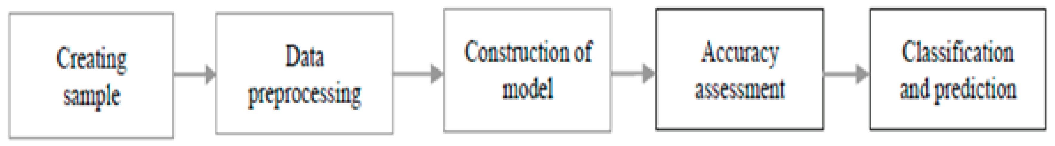
The empirical research for predicting currency crises involved five steps: Creating the sample, data preprocessing, model construction, accuracy assessment, and classification and prediction as shown in Figure 2. The first step (sample creation) was based on obtaining the relevant data from the data sources such as information published by international economic bodies. The attributes of the dataset include measurements of exposure to debt, the external sector, domestic macroeconomic factors, the banking sector, and political attributes. The data preprocessing step involved making the attributes with continuous values discreet, generalizing data and analysis of the relativity of the attributes, and eliminating outlier values. Regarding outliers values, since the deletion of elements of the sample implies a loss of information, only the ends that do not belong to the interval have been suppressed:

(Q₁ − 3R_Q, Q₃ + 3R_Q)

(9)

where Q₁ is the first quartile, Q₃ is the third quartile, and R_Q is interquartile range.

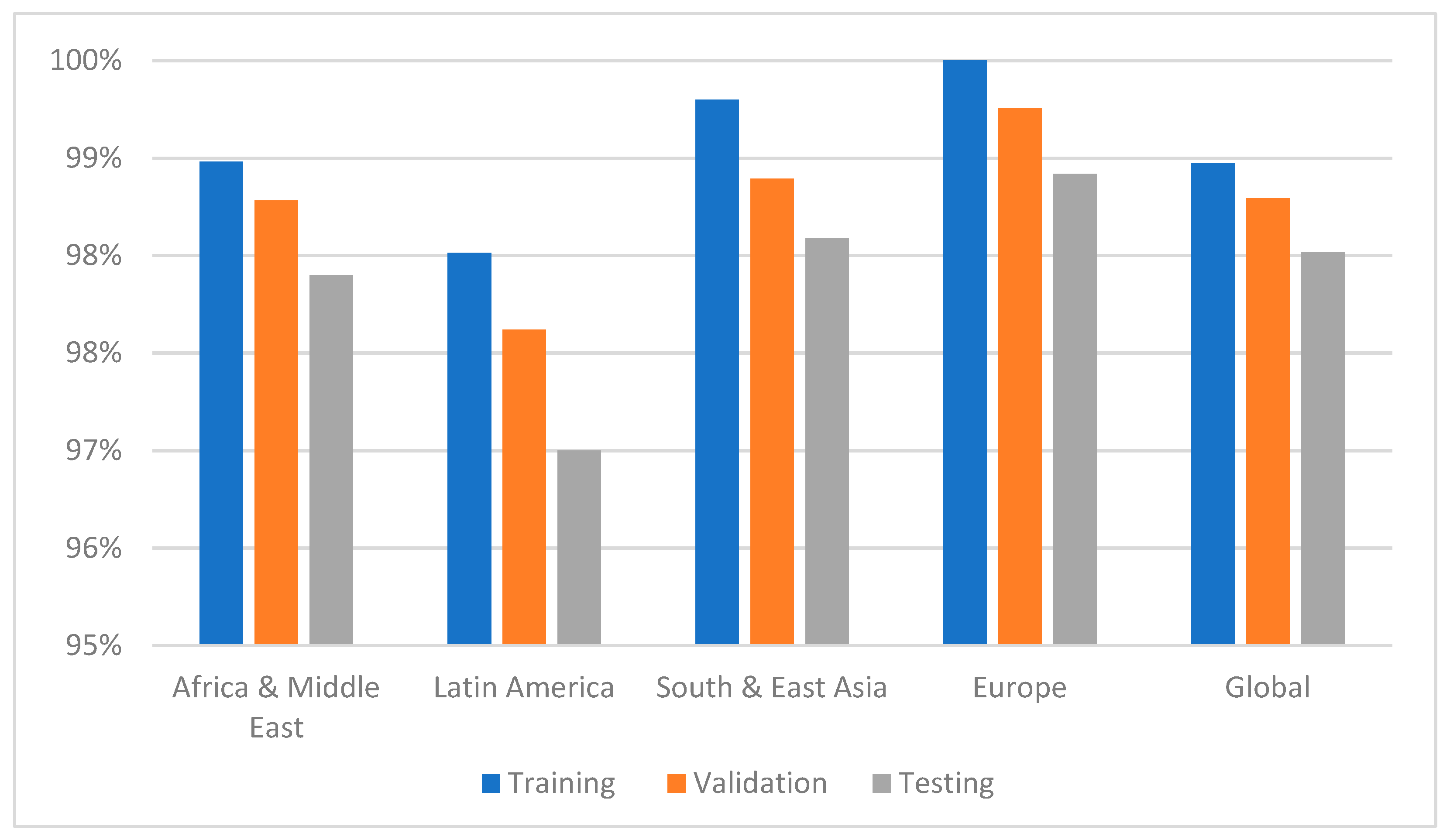
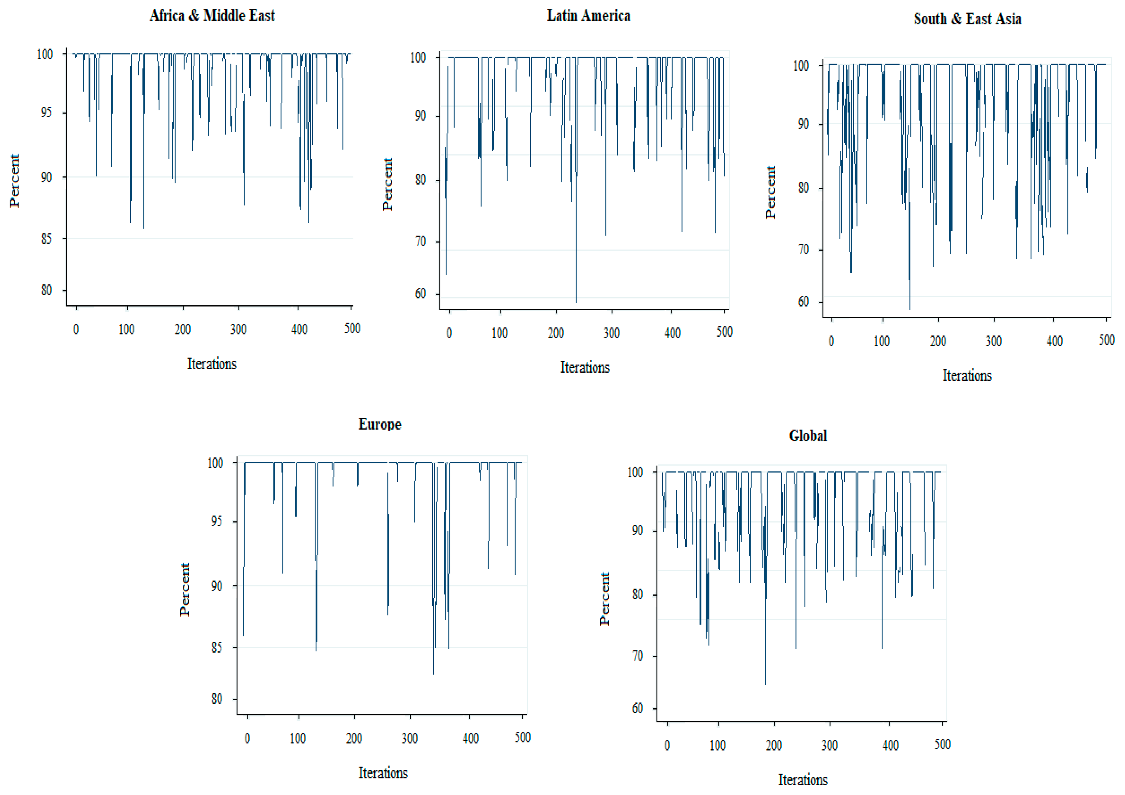
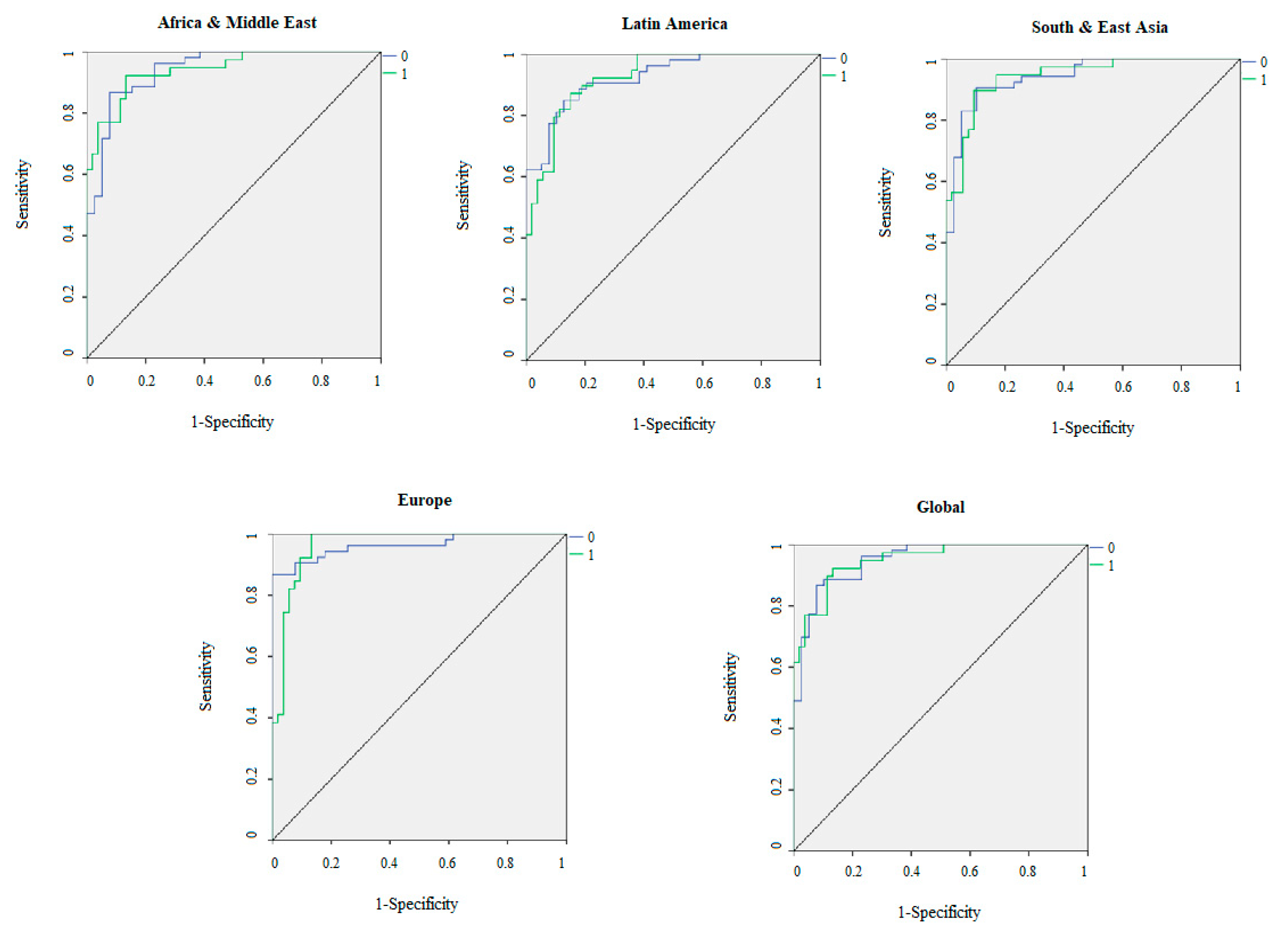
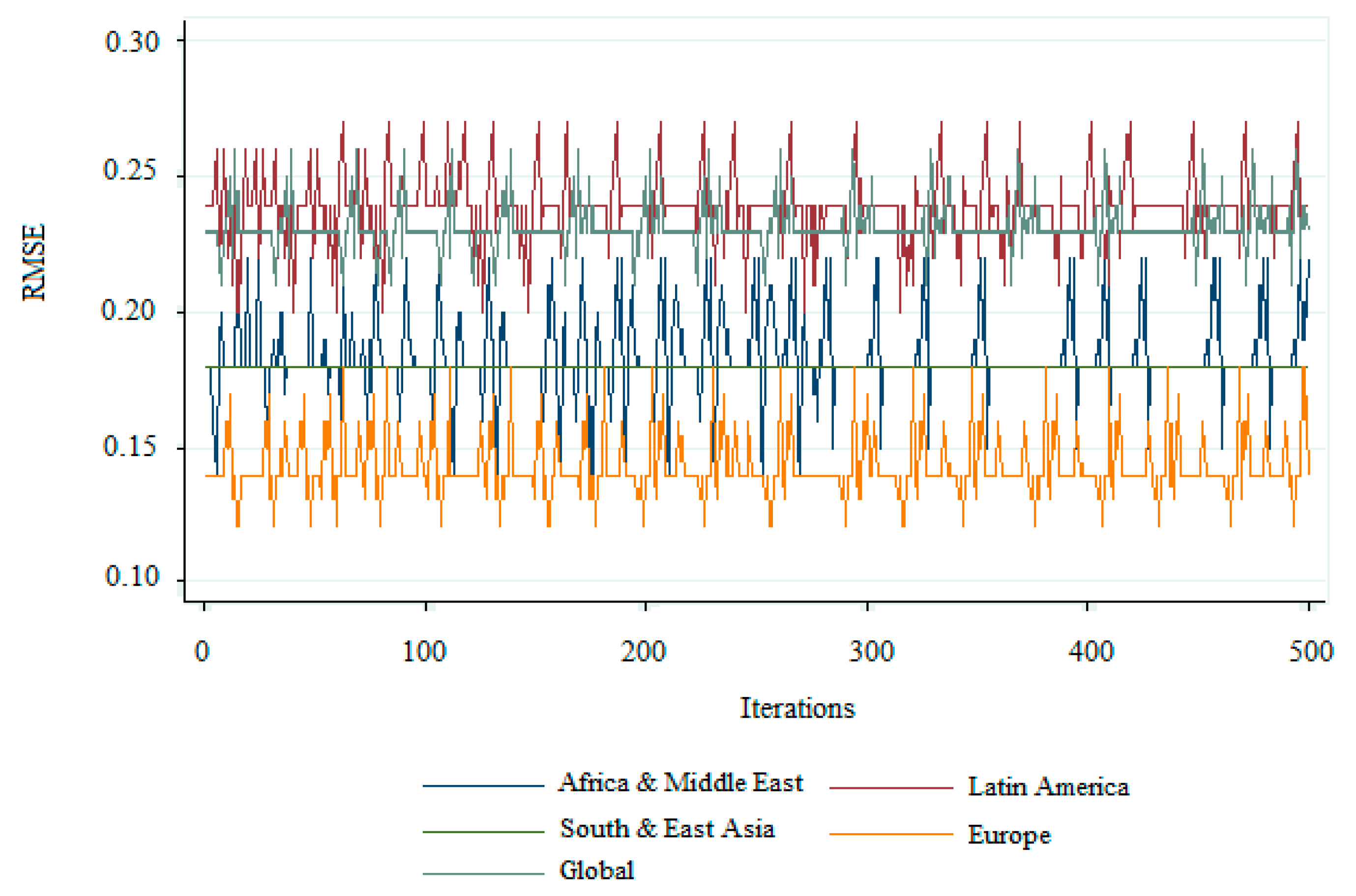
The step of constructing the model was based on inductively learning from the preprocessed data using the DNDT algorithm defined in Section 2 and choosing the significant independent variables via the proposed sensitivity analysis. To do so, the sample was randomly divided into three mutually exclusive datasets: Training (70%), validation (10%), and testing (20%). This process used the 10 fold cross-validation method with 500 iterations to estimate error ratios [37]. The first subset of data was used to train the models and estimating the parameters. The second subset was used for model selection. Finally, the third dataset (testing) was used to evaluate the predictive accuracy of the model in the accuracy assessment step. This was complemented by the analysis of the model’s robustness and its predictive capacity for currency crises at the global level in the classification and prediction step. All variables used in this study were considered in every dataset of training, validation, and testing data

3. Data and Variables

The sample used in this study comprised 162 developed, emerging, and developing countries with information for the period 1970–2017 (Appendix A). The granularity of the data was annual, following the format data of previous works [1,12,38]. The dataset of the present study had 7708 observations, being 236 crisis observations. Specifically, a set of 32 explanatory variables chosen from the existing literature on the prediction of currency crises was obtained. Of these, 23 corresponded to factors related to debt exposure, the external sector, domestic macroeconomy, and the banking sector [1,14,15,17,19]. This information was sourced from the International Monetary Fund (IMF) International Financial Statistics, World Bank Development Indicators, World Economic Outlook, and the World Bank Global Financial Database. The nine remaining variables refer to political factors and have been extracted from the database of the Polity IV Project of Center for Systemic Peace, selecting the variables used in Reference [39]. The dependent variable was constructed based on the definition in Reference [38]: “a currency crisis is defined as a nominal depreciation of the currency with respect to the US dollar by at least 30% and at least 10 percentage points higher than the depreciation rate for the previous year”. This dependent variable was 1 for the years in which currency crises occurred and 0 otherwise. The choice of countries was mainly guided by the availability of data, covering four main regions: Africa and the Middle East, South and East Asia, Latin America, and Europe.

Table 1. Independent variables.

Category	Code	Definition	Expected Sign 1
Debt Exposure	Total Debt	gross external debt as % of GDP	+
	Short-Term Debt	gross short-term external debt as % of GDP	+
	Real Interest Rate	lending interest rate adjusted for inflation	+
External Sector	Foreign Exchange Reserves	total reserves (without gold) as % of GDP	−
	Trade Openness	ratio of exports plus imports to GDP	+/−
	Imports	imports of goods and services at current prices in USD	+/−
	Exports	exports of goods and services at current prices in USD	−
	Current Account	current account balance as % of GDP	−
	Portfolio Investments	portfolio investment net at current USD	−
	FDI	net FDI inflows as % of GDP	−
Domestic Macroeconomic Factors	Real GDP	annual real GDP at current USD	−
	Real GDP Growth	annual growth of real GDP	−
	Inflation	rate of change in CPI	+
	M2 Multiplier Growth	annual growth of M2	+
	M2/Reserves	ratio of M2 to foreign exchange reserves	+
	REER Overall	deviation of real effective exchange rate from 5 year rolling mean	−
	Government Spending	general government final spending as % of GDP	+/−
	Fixed Capital Formation	gross fixed capital formation at current USD	−
	Unemployment	unemployment total as % of total labor force	+
	Contagion	event of a currency crisis in any country of the same region (t − 1)	+
	Soft Peg 2	exchange rate regime applied to currency to keep its value stable against a reserve currency	+
	Peg 2	exchange rate regime in which a currency’s value is fixed against either the value of another country’s currency	+
Banking Sector	Domestic Credit	ratio of domestic credit to GDP	+/−
	Lending Interest Rate	the bank rate meets the short- and medium-term financing needs	−
	Deposit Interest Rate	rate paid by banks for demand, time, or savings deposits	−
Political Factors	Polity	combined polity score (autocracy score minus democracy score)	+/−
	Durable	regime durability (control variable of Polity)	+
	Persist	polity persistence (control variable of Polity)	+
	SFI	state fragility index	+
	Left Government	left-leaning government	+
	Election	legislative/executive election	+
	Turnover	annual turnover of veto players	+
	Years	years in the office of chief executive’s party	+
	Economic Effectiveness	effectiveness of economic policy measured by GDP per capita	−

¹ The expected relationship of the independent variable according to its influence to increase or decrease the probability of suffering a currency crisis. ² It is denoted with 1 when the country applies this exchange rate regime for the year under consideration and 0 otherwise.

shows the independent variables used in this research.

4. Results

4.1. Descriptive Statistics

The main descriptive statistics for the variables of the sample are provided in

Table 2. Descriptive statistics.

Variables	Dependent Variable
	0		1
	Mean	SD 2	Mean	SD 2
Total Debt	57.219	12.565	63.814	16.204
Short-Term Debt	10.381	7.053	13.725	7.824
Real Interest Rate	5.763	2.422	7.416	2.942
Foreign Exchange Reserves	9.608	8.642	17.522	13.458
Trade Openness	61.517	7.874	56.174	7.273
Imports 1	51,856	344.565	16,418	245.637
Exports 1	53,783	387.632	16,976	265.484
Current Account	−2.578	1.206	−2.533	1.384
Portfolio Investments 1	−2.123	362.859	−114,665	154.350
FDI	1.959	1.362	4.019	2.548
Real GDP 1	1,950,090	78,250.933	69,591	4527.409
Real GDP Growth	4.157	1.594	0.705	1.062
Inflation	18.495	7.452	37.820	9.781
M2 Multiplier Growth	0.125	0.126	0.272	0.151
M2/Reserves	485.463	24.572	502.848	26.287
REER Overall	112.772	21.783	85.259	18.523
Government Spending	15.589	9.747	24.171	11.083
Fixed Capital Formation 1	56,025	276.574	17,199	127.496
Unemployment	9.365	7.842	14.046	11.578
Contagion	0.138	0.035	0.192	0.370
Soft Peg	0.164	0.042	0.249	0.076
Peg	0.089	0.017	0.135	0.051
Domestic Credit	52.768	17.478	73.721	19.779
Lending Interest Rate	34.048	16.675	22.463	14.347
Deposit Interest Rate	37.617	18.428	42.843	23.362
Polity	−1.000	0.426	−5.000	0.618
Durable	24.000	2.165	11.000	1.482
Persist	17.000	2.478	9.000	1.247
SFI	5.000	1.822	12.000	2.151
Left Government	0.412	0.237	0.574	0.428
Election	0.096	0.057	0.126	0.084
Turnover	5.590	1.573	5.460	1.522
Years	7.693	2.582	2.942	2.165
Economic Effectiveness	2.000	1.562	1.300	1.257

¹ Variables expressed in millions of USD. ² Standard deviation.

. Episodes of currency crises (dependent variable = 1), compared to the absence of these episodes (dependent variable = 0), are characterized by higher average levels of public debt (Total Debt and Short-Term Debt), less openness to the rest of the world (Trade Openness, Imports, and Exports), and alarming results in certain macroeconomic indicators like Real GDP Growth and Inflation. In contrast, the remaining variables have lower average values. There is also a moderate dispersion in the distribution of the variables analyzed which can be extended to the sample as a whole.

4.2. Estimated Models

Table 3. Comparison of accuracy ratios of deep neural decision trees (DNDTs) with other methodologies.

Model	Dataset	Logit	Multilayer Perceptron	Support Vector Machines	AdaBoost	DNDT
Africa and Middle East	Training	91.52	94.44	93.38	95.25	99.17
	Validation	90.84	93.91	92.57	94.57	98.85
	Testing	90.25	93.62	92.18	94.11	98.24
Latin America	Training	91.16	94.12	93.04	95.08	98.42
	Validation	90.72	93.37	92.68	94.21	97.79
	Testing	90.20	92.85	91.95	93.36	96.90
South and East Asia	Training	91.64	95.06	93.47	96.17	99.68
	Validation	91.03	94.52	93.02	95.64	99.03
	Testing	90.62	94.13	92.61	95.19	98.54
Europe	Training	92.19	95.43	93.81	96.86	100.00
	Validation	91.58	95.10	93.22	96.42	99.61
	Testing	90.88	94.46	92.93	95.73	99.07
Global	Training	91.59	94.84	93.33	95.95	99.16
	Validation	90.94	94.27	92.65	95.34	98.87
	Testing	90.37	93.76	91.83	94.28	98.43

shows the levels of precision (in percentage) reached in the classification of the currency crises of the methodologies applied in the present study for the three data sets: Training, validation, and testing. In greater order to less accuracy, it is shown that in all models, the DNDT method was the one that achieved greater classification capacity, followed by AdaBoost, MLP, SVM, and Logit.

Figure 3 shows the results obtained using DNDTs for the models in each region and the global model. The classification accuracy obtained using the training data was 99.17%, 98.42%, 99.68%, 100%, 99.16% for the models for Africa and Middle East, Latin America, South and East Asia, Europe, and Global, respectively. The accuracy obtained using the validation was 98.85%, 97.79%, 99.03%, 99.61%, and 98.87% for the models for Africa and Middle East, Latin America, South and East Asia, Europe, and Global, respectively. Finally, the accuracy for the testing data was 98.24% for Africa and Middle East, 96.90% for Latin America, 98.54% for Asia, 99.07% for Europe, and 98.43% for the Global model. Figure 4 shows the accuracy rates obtained for each model in the 500 calculation iterations.

The goodness-of-fit for the models developed was measured by both the corresponding ROC curves and root mean square error (RMSE). The area of the ROC curve for the five models was close to 1, indicating satisfactory levels in all cases (Figure 5). The RMSE for the 500 iterations in the estimations with the test data is shown in

Table 4. The root mean square error (RMSE) scores of estimated models.

Model	RMSE
	Training	Validation	Testing
Africa and Middle East	0.13	0.15	0.19
Latin America	0.21	0.25	0.24
South and East Asia	0.12	0.16	0.18
Europe	0.09	0.12	0.14
Global	0.18	0.21	0.23

and Figure 6. The RMSE was less than 0.30 in all models, also showing a close fit for all models.

Figure 7 shows the most significant variables for each model in line with the sensitivity analysis (Appendix B shows the sensitivity of all the variables). The results show a group of significant variables that are repeated in practically all the estimated models. The variable Fixed Capital Formation was significant in all models, showing the significance of the change in the net investment of a country for the risk of a currency crisis. This result contradicts the previous experience in Reference [40], for which this variable was not significant. Regarding the domestic macroeconomic variables, those for monetary supply (M2 Multiplier Growth and M2/Reserves) were also highly significant, showing that a surge in money supply was detrimental to the currency price (also corroborated by the sensitivity of the variable REER Overall in the majority of models). Similarly, variables for the External Sector attribute, such as Trade Openness, FDI and Current Account, were highly sensitive, indicating the significance of the behavior of a country’s international trade on its currency price. This is in contrast to the findings of previous studies [1,15,41]. Similarly, the variables Total Debt and Government Spending (related to the accumulation of debt) were also highly significant, showing that high public debt ratios increase the risk of currency crises. Finally, the most significant political variables in our models were SFI (Latin America and Global), which shows the capacity of the government to make and implement public policy, and Polity which indicates the level of democracy of a country. Existing literature has not found these political variables to be significant [39]. The results also differ in terms of the variables for the banking sector which have been significant in previous work [6,7] but which did not exhibit a high level of sensitivity in our estimations.

The results of this study confirm that the models developed using DNDTs obtained a predictive capacity of nearly 100% for currency crises in both regional models and the global model, obtaining higher levels of accuracy than previous studies. The accuracy of the global model was 96.38%, although a comparison of this model is difficult, since it is the first model created to protect currency crises at the global level. Other studies have obtained lower levels of accuracy than our results, such as Reference [6], which obtained an accuracy of 84.62% using the dynamic panel model. Similarly, we also improved on the results obtained by Reference [16] which obtained 93.8% accuracy using NN for Turkey. Our methodology also had greater predictive power than other computational techniques like kNN-SVM, which obtained 97% accuracy for a sample of emerging countries [1] and random forests and wavelet transform, recently applied in Reference [42] to a sample of emerging and underdeveloped countries (ROC value = 0.94).

5. Conclusions

Currency crises constitute an area of international concern that has received interest from macroeconomic researchers and public policymakers in recent decades. Our results show that DNDTs improve the accuracy of predictive models for currency crises. They also improve the quality of information for policymakers in the regions under consideration who require empirical tools to mitigate and resolve the impact of a sharp fall in the value of their currency and the negative effects. Our models may also be of particular relevance to financial institutions, such as rating agencies and central banks, which need to control the risk of a potential imminent crisis.

The DNDT algorithm exhibited high predictive capacity in the case analyzed as a result of using NNs to implement DTs. The algorithm also improved the interpretation of results and the quality of information. The results are more accurate than in the existing literature, taking into account the requirement of the samples used in this study.

The results of this study have also suggested a new set of variables to predict currency crises. In this respect, the significance of variables for the external sector and domestic macroeconomy stands out, suggesting they are the best indicators to predict a currency crisis at the global level. There are also a number of other variables for models adapted to the specific circumstances of Asia and Europe, and Africa and Latin America, in which the political and domestic credit variables stand out.

Given the significance of the issue addressed in this study, presenting a global forecasting model to address a gap in the existing literature and obtaining accuracy in the testing sample of over 96% represents significant progress in the challenging task of forecasting future currency crises. It also provides a unique international experience, simplifying and reducing the resources and effort for creating different models for predicting currency crises.