Optimal Scheduling of Residential Home Appliances by Considering Energy Storage and Stochastically Modelled Photovoltaics in a Grid Exchange Environment Using Hybrid Grey Wolf Genetic Algorithm Optimizer

Abstract

The transformation of a conventional power system to a smart grid has been underway over the last few decades. A smart grid provides opportunities to integrate smart homes with renewable energy resources (RERs). Moreover, it encourages the residential consumers to regulate their home energy consumption in an effective way that suits their lifestyle and it also helps to preserve the environment. Keeping in mind the techno-economic reasons for household energy management, active participation of consumers in grid operations is necessary for peak reduction, valley filling, strategic load conservation, and growth. In this context, this paper presents an efficient home energy management system (HEMS) for consumer appliance scheduling in the presence of an energy storage system and photovoltaic generation with the intention to reduce the energy consumption cost determined by the service provider. To study the benefits of a home-to-grid (H2G) energy exchange in HEMS, photovoltaic generation is stochastically modelled by considering an energy storage system. The prime consideration of this paper is to propose a hybrid optimization approach based on heuristic techniques, grey wolf optimization, and a genetic algorithm termed a hybrid grey wolf genetic algorithm to model HEMS for residential consumers with the objectives to reduce energy consumption cost and the peak-to-average ratio. The effectiveness of the proposed scheme is validated through simulations performed for a residential consumer with several domestic appliances and their scheduling preferences by considering real-time pricing and critical peak-pricing tariff signals. Results related to the reduction in the peak-to-average ratio and energy cost demonstrate that the proposed hybrid optimization technique performs well in comparison with different meta-heuristic techniques available in the literature. The findings of the proposed methodology can further be used to calculate the impact of different demand response signals on the operation and reliability of a power system.

1. Introduction

The increasing costs of energy and environmental contamination are major concerns in today’s world [1]. As most of the power plants rely on fossil fuel resources for electricity production, they are depleting at a fast rate. Moreover, the increased utilization of fossil fuels is resulting in global warming, which is a challenging issue to deal with. These seminal drivers have led to the belief that the need for public and private decision-makers to transition toward green and sustainable energy is inexorable. The integration of renewable energy resources (RERs), especially solar and wind, is a handy option for generating green electricity with reduced global warming effects [2,3].

These factors lead us to the concept of a smart grid, which is a digital, bidirectional network of distributed generators. Due to installed sensors, it has the capabilities of self-monitoring, self-healing, remote control, and pervasive control [4,5]. A smart grid offers opportunities for maximum energy savings by organizing energy management systems (EMSs) and their functions. It relies on intelligent control devices to establish an efficient communication between the consumer and utility provider.

Mutual coordination between electric grids, utility operators, and smart homes is the main point that allows a smart grid to work accurately. A major part of electrical energy is being utilized for serving residential communities. According to Lior [6], 30–40% of the overall supplied energy is used in residential houses. Therefore, energy management in residential homes plays an important role in reducing the consumption of electrical energy supplied by the grid to diminish the peak load on grids. With the improvement in control and communication methodologies, home energy management systems (HEMSs) are playing an important role in reducing electricity consumption in residential buildings. An optimal collaboration between smart homes and the utility provider due to HEMS decreases electricity consumption cost [7].

Moreover, an optimum collaboration between smart homes and a smart grid saves 10–30% of electrical energy consumed from the grid [8]. Electricity providing utilities introduced different dynamic tariff structures to encourage the electricity customers to decrease their consumption in high-tariff time slots [9,10]. Based on this information, a smart grid utilizes supply-side management (SSM) and demand-side management (DSM) tools for energy conservation. The optimization activities covered in SSM are implemented regarding the generation, transmission, and distribution sides of the energy chain, while in DSM, the consumer side load management is performed based on the demand response. The electricity consumption charges may be reduced by shifting household appliances from a peak tariff time to an off-peak tariff time.

The users can get maximum benefits in terms of a decrease in electricity consumption charges, reduction in the peak-to-average ratio (PAR) and avoiding energy blackouts due to two features of DSM, namely the demand response (DR) and load management (LM) [11]. DR programs play a significant role in a smart grid operation by scheduling household appliances from away from high-tariff time slots to low-tariff time slots according to time-based electricity tariffs, which are explained in References [9,12].

DR programs are further classified into two types, i.e., incentive-based (IB) and price-based (PB) DR programs. Figure 1 represents the classification of DR programs.

In IB DR programs, the utility wirelessly shifts home appliances to an OFF state by sending a short notice to consumers whenever a peak demand occurs in any time slot [13]. Using the PB DR programs, the electricity utilities encourage the electricity users to adopt efficient scheduling strategies such that they can minimize their electrical energy consumption and reduce their electricity consumption costs [14].

This paper focuses on PB DR programs with the integration of RERs, and energy storage system (ESS), and a smart meter at each home. The smart meter continuously provides information related to hourly tariffs that are declared by the electricity provider to the consumer. Due to this, the electricity users schedule their hourly load according to the declared utility tariffs. This hourly electricity load management is useful for both electricity consumers and electricity providers in terms of reducing electricity consumption costs and improving the stability of the power system.

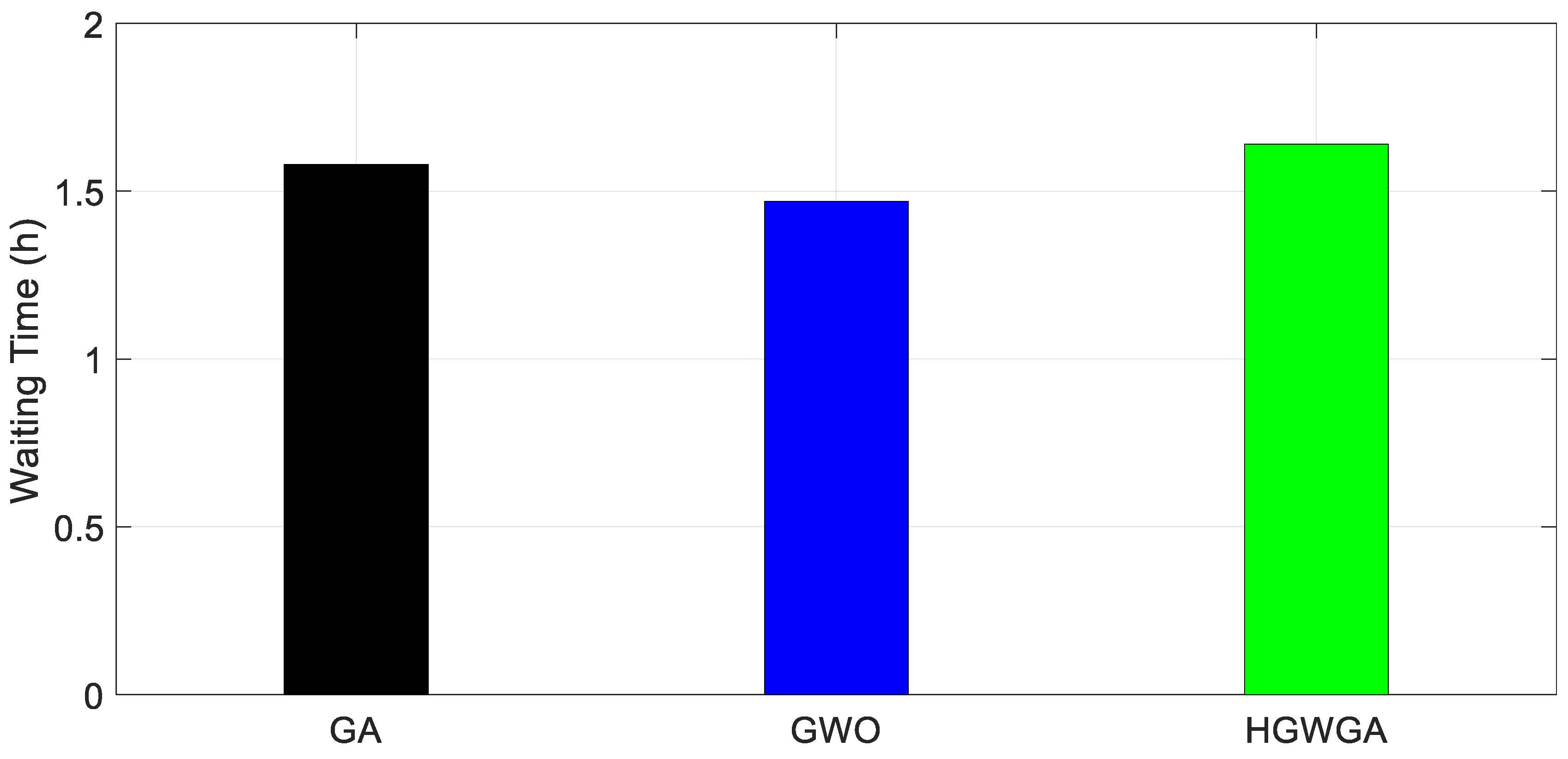
In the proposed HEMS scheme, an ESS and photovoltaic (PV) generation system were further integrated to improve the performance of the primitive HEMS. Three optimization algorithms, i.e., a genetic algorithm (GA); grey wolf optimization (GWO); and the proposed hybrid technique based on GWO and GA, named a hybrid grey wolf genetic algorithm (HGWGA), that considers real-time pricing (RTP) and critical peak pricing (CPP) tariff schemes, were used to solve the scheduling problem. Simulation results demonstrate that the proposed hybrid optimization technique performed well at reducing the PAR and consumption costs of electricity. However, there is always a trade-off between consumer electricity consumption cost and consumer appliance waiting time (AWT). Whenever the consumer electricity consumption cost was at a minimum, the consumer AWT was at a maximum and vice versa.

Contributions

The main contributions of this paper are:

• The application of a hybrid optimization technique (HGWGA) to effectively solve the appliance scheduling problem.
• The integration of stochastic models of ESS, a PV system, and loads for optimal scheduling.
• The investigation of RTP and CPP tariffs using the proposed model for optimal scheduling.

The rest of the paper is organized in the following manner. Section 2 presents a technological review of the literature, while in Section 3, mathematical models of a HEMS are discussed. Section 4 formulates the load scheduling problem by discussing issues regarding consumer energy consumption, electricity consumption cost, PAR, AWT, and the objective function. The heuristic optimization techniques implemented to solve the scheduling problem are explored in Section 5. Section 6 and Section 7 contain the case studies and simulations results, respectively, while Section 8 summarizes the paper with concluding remarks.

2. Literature Review

The optimal scheduling of smart home appliances is a challenging problem that is focused on by many researchers. The main objective is to minimize the consumption cost of electricity and achieve a load balance among the supply and demand sides. In the last few decades, several methodologies and techniques have been proposed by researchers for minimizing users’ electricity consumption cost, reducing the PAR, and maximizing the consumers’ comfort.

The optimum scheduling and operation of home appliances is a non-linear, discrete, and multi-dimensional problem with multiple constraints. Several traditional, evolutionary, and swarm intelligence techniques, such as mixed-integer programming (MILP), real-time rolling optimization (RTRO), bat algorithm (BA), GWO, and particle swarm optimization (PSO), etc., are considered in the literature to solve the home appliance scheduling problem [15,16].

Zhang et al. [17] proposed a scheduling strategy using MILP to optimally operate household appliances for achieving a reduction in the emission rate, energy import from the grid, and financial burden on the user. Bradac et al. [18] presented a scheduling technique to minimize the electricity consumption cost with a PAR reduction for residential consumers in peak hours using MILP. However, their proposed model did not consider consumers’ comfort.

Huang et al. extended the work presented in Bradac et al. [18] using heuristic techniques for reducing residential energy consumption during peak hours and cost minimization while incorporating consumers’ comfort as well [19]. Lokeshgupta and Sivasubramani [20] proposed an optimal strategy for a HEMS with the objectives of cost minimization and peak load reduction while incorporating an energy storage system (ESS). A MILP technique was used to solve this multi-objective problem for residential customers using a time-of-use (ToU) pricing scheme that offers low prices during the off-peak and the mid-peak hours while offering high prices during the peak hours. The integration of RERs was not considered in their proposed scheme.

Kuzlu [21] presented a score-based intelligent home energy management algorithm for attaining the optimum scheduling of home appliances by considering an electricity purchase tariff and the PAR. RERs and ESS were not considered in their proposed model.

A GA-based model of a HEMS was proposed in Mohamed and Koivo [22] with the purpose of reducing the consumption cost of electricity for residential consumers. Models based on evolutionary algorithms were proposed in References [23,24] to solve an energy-based optimization problem in a residential area. In the proposed models, authors presented a strategy for the scheduling of household appliances in different time intervals to minimize electricity consumption expenses and the PAR. However, the integration of RERs and an ESS were not considered in these models.

A PSO is a swarm intelligence algorithm that is frequently implemented for the optimal scheduling of the HEMS [25]. Rehman et al. developed a binary PSO (BPSO) algorithm in Rehman et al. [26]. Their proposed algorithm automatically controlled the appliance scheduling by shifting the consumers’ load from a high-pricing time to a low-pricing time. Since a PSO is appropriate for solving real number optimization problems, it might get stuck in a local optimum value in discrete optimization problems. HEMS is a discrete problem; therefore, a PSO algorithm is not suitable for this type of problem [27].

Liao et al. [28] proposed an electron drifting algorithm (EDA) to optimally operate household appliances for achieving a reduction in the emission rate, energy import from the grid, and financial burden on the user. The main strength of the proposed EDA compared to other algorithms was its lower probability of getting stuck in a local minimum. However, this algorithm lacks the availability of explicit rules for constraints handling, which results in a high uncertainty.

Javaid et al. [29] applied a GA, BPSO, and a Cuckoo search optimization algorithm (CSOA) to develop an optimal scheduling strategy for residential appliances in the presence of an ESS and RERs. The objective of the implemented idea was to reduce the consumers’ electricity cost under a ToU tariff scheme and minimize the PAR.

Basit et al. [30] presented a model to solve an appliance scheduling problem by using the Dijkstra algorithm and reducing the system complexity. Integration of the ESS and RERs were not considered in their proposed model.

The minimization of the consumption cost of electricity in a smart grid environment using an evolutionary technique was discussed in Mary and Rajarajeswari [31] through the integration of an ESS. During a low electricity tariff time, energy was stored in the ESS and it was utilized during the peak-tariff time. Charging and discharging limits of the battery per time slot were also defined by the authors to avoid battery damage. However, the authors did not consider the installation cost of the storage system.

An innovative technique was proposed in Bharathi and Vijayakumar [32] to keep the supply demand balance in residential, commercial, and industrial areas. The authors compared the electrical consumption of different residential consumer’s datasets via a GA-assisted DSM and a simple DSM. Simulation results demonstrated that a DSM with a GA (DSM-GA) gave better results than a DSM without GA. The PAR and consumer comfort were not considered by the authors in their proposed model.

Asgher et al. presented a strategy for residential load management with the integration of RERs [33]. Their proposed scheme used a GA to optimally schedule the load demand using a day-ahead pricing (DAP) tariff to meet the cost-minimization and PAR-reduction objectives.

Sharifi and Maghouli [34] proposed a novel scheduling mechanism for home appliances to reduce the consumption costs and the PAR. The scheduling model is implemented in inclined block rate (IBR) and real-time pricing schemes to avoid a peak demand during low-tariff times, which would improve the PAR index as well. A non-dominated sorting genetic algorithm (NSGA) was adopted to solve the optimization problem in a MATLAB simulation environment.

Aslam et al. [35] proposed a scheduling technique for minimizing the residential consumer electrical energy consumption and reducing the PAR with the help of the heuristic techniques of a GA, CSOA, and a Crow search algorithm (CSA) under RTP and CPP tariff schemes. However, the integration of RERs was not considered in their proposed model.

Hafeez et al. [36] formulated a scheduling problem for residential consumer home appliances using a GA, BPSO, wind-driven optimization (WDO), and hybrid framework of a GA and WDO. The minimization of the electricity consumption cost and the decrease in the PAR were the main objectives in the RTP and inclined block rate (IBR) tariff schemes. The simulation results demonstrated that the above-mentioned methodology achieved the defined objectives in an effective way. However, in the proposed scheme, the authors did not consider the H2G energy exchange environment.

Tsui and Chan [37] developed a scheduling scheme for residential consumer home appliances using convex programming (CP) to minimize the electricity consumption cost and decrease in the PAR. In this model, the RTP tariff scheme was used for the calculation of the electricity consumption cost. It can be concluded from the results that the proposed model is able to effectively achieve the objectives.

To maintain the balance between the residential electrical energy demand and supply, a fuzzy logic (FL)-based model is presented in Wu et al. [38]. An ESS and PV system are also integrated in their scheduling scheme. The proposed scheme has the ability to schedule the home appliances, ESS, and PV in an optimal way.

Naz et al. [39] applied an enhanced differential evolution algorithm (EDEA), GWO, and a hybrid framework of EDEA and GWO to develop an optimal scheduling strategy for residential appliances in the presence of an ESS and RERs. The implemented idea was to minimize the consumer electricity cost and reduction in the PAR under RTP and CPP tariff schemes.

Khan et al. [40] designed a scheduling problem for residential consumer home appliances by using a harmony search algorithm (HSA), EDEA, and a hybrid framework of HSA and EDEA. The minimization of the electricity consumption charges and decrease in the PAR were the main objectives. In this model, the RTP tariff scheme was used for the electricity consumption cost calculation. Simulation results demonstrated that the above-mentioned methodology achieved the defined objectives in an effective way.

Setlhaolo et al. [41] developed a model for residential consumers to diminish their electricity consumption charges under a ToU tariff scheme. They applied a mixed-integer non-linear programming (MINLP) scheme without considering the PAR in their proposed model.

An integer linear programming (ILP) scheme was proposed for residential areas in Zhu et al. [42] to meet the supply–demand balance objective while reducing the consumption cost of electricity. Since the proposed scheme could schedule the home appliances in an optimal way, the supply–demand balance goal was achieved after the optimal scheduling of household appliances for several consumers. This study ignores the users’ comfort in the modeling.

A dynamic programming (DP)-based appliance scheduling model is proposed in Samadi et al. [43] for the optimal shifting of consumers’ household appliances in a defined time interval by considering the appliance preferences set by the consumers. The main aim of this scheduling strategy was to decrease the consumer electricity consumption charges by rescheduling consumer home appliances from a high-tariff time interval to a low-tariff time interval according to their preferences.

Keeping in mind the above literature, it can be summarized that the design of a HEMS has been optimized by various algorithms: MILP, EDA, linear programming (LP), PSO, DP, convex programming (CP), bacterial foraging algorithm (BFA), score-based intelligent home energy management algorithm, ILP, Dijkstra algorithm, and MINLP. Nevertheless, in some scenarios, these techniques are unable to deal with the volatile nature of different appliances. Furthermore, the convergence rate in some cases was found to be extremely slow because these algorithms were often stuck in local minimum solution. Some important practical constraints, such as the maximization of user comfort, dynamic pricing scheme, and the integration of an ESS and RERs, are somehow rarely considered while using such techniques. In addition, previously proposed models were based on the deterministic modeling of the load, ESS, and RERs. As RERs, such as solar and wind, are weather-dependent, the energy produced by these resources is variable and uncertain. This variability is generally modeled through stochastic or probabilistic approaches. Therefore, this paper presents an optimal design of a HEMS incorporated with the probabilistic modeling of the loads, ESS, and PV by considering RTP and CPP tariff schemes to provide a reduced consumption cost and a better consumption pattern, which indicates reduction in PAR using a GWO, GA, and the proposed hybrid (HGWGA) technique.

3. System Architecture

The proposed architecture of a HEMS consists of an energy management controller (EMC), smart meter, display system, smart scheduler unit (SMSU), PV system, ESS, power electronic converter, and a set of appliances. A power electronic converter serves the purpose of a rectifier and inverter. The smart appliances, PV system, and ESS are connected to the EMC and SMSU through a wireless system in this research. The smart meter is connected to the SMSU and receives RTP and CPP tariff signals through an advanced metering infrastructure (AMI). Based on the received tariff signals and the operating preferences set by the user regarding appliance operations, the SMSU employs heuristic optimization algorithms to find the optimal scheduling of appliances that results in reduction of energy cost as well as the peak demand. These scheduling results are transmitted to an EMC, which schedules the home appliances without compromising the consumer’s comfort. The architecture of the proposed model is shown in Figure 2. It is assumed that the H2G energy exchange through a smart meter is allowed. These types of tariffs are normally termed as net-metering or net-billing.

3.1. Smart Homes Appliance Models

For the performance evaluation of the proposed methodology, smart home appliances were classified in three different categories. These categories included deferrable appliances, base load appliances, and non-deferrable appliances. The total number of user appliances was represented by $A_n$. Deferrable appliances, base load appliances, and non-deferrable appliances were represented by $A_d$, $A_b$, and $A_{nd}$, respectively. According to the user requirements and preferences, all user appliances were scheduled with a 24-h time horizon, as expressed in Equation (1).

$$h\in H \forall H=\left\{h_1,h_2,h_3,\dots ,h_{24}\right\}.$$

(1)

The execution period for each appliance should be within the earliest starting time (ἀ) and least finishing time ($\stackrel{`}{\beta }$), as represented in Figure 3. The difference between the earliest starting time and the actual starting time is known as the waiting time of the individual appliance. ἀ and $\stackrel{`}{\beta }$ for individual appliances were circumscribed by the consumer, as described in

Table 1. Genetic algorithm (GA) parameters.

Parameters	Value
Population size	200
Number of iterations	100
Probability of crossover	0.9
Probability of mutation	0.1
Number of appliances	12

. In the proposed home appliance scheduling scheme, twelve different rudimentary appliances were considered for a smart home, which are mentioned in Table 1.

3.1.1. Base Load Appliances

Base load appliances are in the first category of appliances and run as a base load in a smart home. Their operating time cannot be changed; however, these appliances can be scheduled between their starting and ending time as defined by the consumer. $a_b\in A_b$ represents any appliance belonging to the base load category of appliances. The total energy consumption utilized by base appliances belonging to set $A_b$ during any time slot $h$ is given by $E_b$ in Equations (13) and (14).

3.1.2. Deferrable Appliances

The household appliances in this category can be interrupted or shifted in any allowable time range according to their requirements for achieving the optimal scheduling in a smart home. The set of deferrable appliances is represented by $A_d$, and $a_d\in A_d$ denotes each appliance in this category. The total energy consumed by all the appliances of this category is represented by $E_d$ in Equations (13) and (14).

3.1.3. Non-Deferrable Appliances

The category of household appliances that cannot be interrupted after the beginning of their operation are non-deferrable appliances. However, these appliances can be shifted in their allowable time range before starting their action in such a way that their operating cycle could be complete after shifting. The set of non-deferrable appliances is represented by $A_{nd}$, $a_{nd}\in A_{nd}$ represents each appliance in this category, and the total electricity energy consumed by non-deferrable appliances at any hour h of a day is given by $E_{nd}$ in Equations (13) and (14).

3.2. Electric Storage System Model

These days, the electrical energy storage devices are playing a significant role in maintaining the system reliability, enhance the power quality (PQ), and achieve green energy goals. Therefore, an ESS was installed for storing electrical energy in the proposed model to improve the performance of the HEMS. When the electricity prices were low, the ESS stores form the utility or excess PV energy.

In this section, the battery ESS was modelled and integrated with the proposed system. The stored energy of battery $E_{bat}\left(h\right)$ in any time interval is presented in Equation (2). A positive value of $E_{bat}\left(h\right)$ represents the charging state of the battery and its negative value denotes the discharging state. The battery charging and discharging efficiencies are represented by ${\eta }_{ch}$ and ${\eta }_{dch}$, respectively. To avoid the rapid charging and discharging of the battery, the constraints given in Equations (3) and (4) should be meet. Equation (3) represents the maximum charging limit and Equation (4) represents the minimum discharging limit of a battery in any scheduling time interval. $S_{bat}$ is a binary variable to represent charging state ($S_{bat}=1)$ and discharging state ($S_{bat}=0)$ of the battery during any hour h of a day.

$$E_{bat}\left(h\right)=\frac{E_{bat}^{ch}\left(h\right)}{{\eta }_{ch}}\cdot S_{bat}\left(h\right)-E_{bat}^{dch}\left(h\right)\cdot {\eta }_{dch}\cdot \left(1-S_{bat}\left(h\right)\right)$$

(2)

$$0\le \frac{E_{bat}^{ch}\left(h\right)}{{\eta }_{ch}}\le E_{ch}^{ max }.S_{bat}\left(h\right)$$

(3)

$$0\le E_{bat}^{dch}\left(h\right)\cdot {\eta }_{dch}\le E_{d_{C}h}^{ max }.\left(1-S_{bat}\left(h\right)\right)$$

(4)

$$SOC\left(h\right)=SOC\left(h-1\right)+ \frac{\left(E_{bat}^{ch}\left(h\right)-|E_{bat}^{dch}\left(h\right)|\right)\cdot h}{C^{battery}}$$

(5)

$$SO{C}_{min} <SOC\left(h\right)< SO{C}_{max}$$

(6)

Equation (5) indicates the battery state of charge $SOC$ and Equation (6) represents the maximum and minimum limits of battery SOC in each time slot. $E_{\mathrm{bat}}^{\mathrm{ch}}\left(h\right)$ and $E_{\mathrm{bat}}^{\mathrm{dch}}\left(h\right)$ signify the charging and discharging state, respectively, of a battery in time slot h.

3.3. PV Generation Model

RERs like wind, tidal biogas, geothermal, and biomass are costly and are not available everywhere. However, PV energy is less expensive and available everywhere. Therefore, the smart home considered in this study was assumed to have its own rooftop PV generation system.

This study used an already developed probabilistic model based on a beta distribution for the modeling of solar irradiance and PV pattern generation, as reported in References [44,45]. Historical irradiance data for a complete year was used for the modeling and generation of PV patterns, and then, these generated patterns were used as the input in this study. The probability density function (PDF) of the solar irradiance $\mathsf{Ɠ}$ is described by the following Equation (7):

$$f\left(\mathsf{Ɠ}\right)=\left(\frac{\gamma \left(\alpha +\beta \right)}{\gamma \left(\alpha \right)\gamma \left(\beta \right)}\right)\times {\mathsf{Ɠ}}^{\left(\alpha -1\right)}\times {\left(1-\mathsf{Ɠ}\right)}^{\left(\beta -1\right)}, 0<\mathsf{Ɠ}\left(t\right)<\infty ,$$

(7)

where $\mathsf{Ɠ}$ is the solar irradiance in kW/m²; $f\left(\mathsf{Ɠ}\right)$ is the beta distribution function of $\mathsf{Ɠ}$; and $\alpha ,\beta$ are the parameters of the beta distribution function. These parameters are computed from the standard deviation $\sigma$ and mean $\mu$ of the random variable $\mathsf{Ɠ}$:

$$\beta =\left(1-\mu \right)\times \left(\frac{\mu \times \left(1+\mu \right)}{{\sigma }^2}-1\right),$$

(8)

$$\alpha =\frac{\mu \times \beta }{1-\mu }.$$

(9)

The output power of the PV panel installed in the proposed smart home was calculated using Equations (10)–(12), as reported in Sajjad et al. [46]:

$$P_{ac}\left(h\right)=0.92\times P_n\times \mathsf{Ɠ}\left(h\right)\times {\eta }_{DC-AC}\times ℰ/1000,$$

(10)

$$ℰ=\left(1-\gamma \times \Delta T_c\left(h\right)\right),$$

(11)

$$\Delta T_c\left(h\right)=\left|25-\left(T_d\left(h\right)+\left(NOCT-20\right)\times \mathsf{Ɠ}\left(h\right)/800\right)\right|,$$

(12)

where $P_n$, $\mathsf{Ɠ}\left(h\right)$, $NOCT$, ${\eta }_{DC-AC}$, and $\gamma$ represent the rated power of the PV system (1–100 kW_p), solar irradiance, temperature of the cell operating under normal conditions (45 °C), efficiency of the inverter (95%), and coefficient of the power temperature (0.007), respectively.

4. Problem Formulation

This section describes the mathematical model of the proposed scheme to achieve the optimal scheduling of home appliances with the integration of PV and an ESS in an H2G energy exchange environment. The prime objective of this work is the minimization of the purchasing cost of electricity from the grid and reduction in the PAR.

4.1. Appliance Energy Consumption

In the proposed system model, the consumer appliances were classified as: deferrable appliances $A_d$, base load appliances $A_b$, and non-deferrable appliances $A_{nd}$. The total number of user appliances is represented by $A_n$. According to the user requirements and preferences, all user appliances are scheduled in 24-h time horizon. The total energy consumed by consumer appliances can be mathematically represented as:

$$E_a\left(h\right)=\left(E_b\left(h\right)+E_d\left(h\right)+E_{nd}\left(h\right)\right),$$

(13)

$$E_a\left(h\right)={\displaystyle \sum }_{h=1}^H\left({\displaystyle \sum }_{a_b\in A_b}\left(P_b\ast S_b\left(h\right)\right)+{\displaystyle \sum }_{a_d\in A_d}\left(P_d\ast S_d\left(h\right)\right)+{\displaystyle \sum }_{a_{nd}\in A_{nd}}\left(P_{nd}\ast S_{nd}\left(h\right)\right)\right),$$

(14)

where $E_b\left(h\right)$, $E_d\left(h\right)$, and $E_{nd}\left(h\right)$ are the energy utilized by base load appliances, deferrable appliances, and non-deferrable appliances, respectively, in each time interval. $A_b$, $A_d$, and $A_{nd}$ represent the set of base load appliances, deferrable appliances, and non-deferrable appliances respectively. $P_b$, $P_d$, and $P_{nd}$ denote the power rating of appliances belonging to the base load, deferrable, and non-deferrable appliances, respectively. $S_b$, $S_d$, and $S_{nd}$ represent the on/off status of the appliance belonging to the baseload, deferrable, and non-deferrable appliances, respectively, during any hour h of a day. ON status is represented by 1 while a 0 value denotes an OFF status of an appliance. An additional constraint, represented by Equation (15), should also be added for non-deferrable appliances to ensure the completion of their entire operating cycle after the beginning of their operation in the predefined interval:

$${\displaystyle \sum }_{h=t+1}^{t+k_a}{S}_{nd}\left(h\right)\ge {\gamma }_a\cdot \left[S_{nd}\left(t+1\right)-S_{nd}\left(t\right)\right], t\in \left[{\mathsf{ἀ}}_a-1, {\stackrel{`}{\beta }}_a-k_a\right],$$

(15)

where $k_a$ represents the required time for an appliance to complete its operation or task and ${\gamma }_a$ demonstrates the required number of time intervals for each appliance to complete its operation. Therefore, if any non-deferrable appliance starts its operation at time $t+1$, then it will complete its task in at least $k_a$ hours. ${\mathsf{ἀ}}_a$ shows the earlier starting time of any appliance and ${\stackrel{`}{\beta }}_a$ represents its least finishing time.

4.2. Energy Exchange with the Grid

The per-hour total energy import from the grid or export to the grid is calculated using Equation (16):

$$E_T\left(h\right)= E_a\left(h\right)-E^{PV}\left(h\right)\pm E_{bat}\left(h\right)$$

(16)

where $E_T\left(h\right)$, $E^{PV}\left(h\right)$, and $E_{bat}\left(h\right)$ represent the per-hour total energy import from the grid or export to the grid, energy generated by the PV in each time slot, and the charging and discharging energy of a battery in each time interval, respectively. A positive sign of $E_{bat}\left(h\right)$ is used to represent charging while a negative sign represents discharging.

4.3. Electricity Consumption Cost

Different utility companies are providing unique tariff schemes such as RTP, CPP, ToU, etc., for their consumers related to their energy import or export in a grid exchange environment. In this work, it was assumed that the tariff for per-hour H2G energy export was half of the rate of the energy import from grid to home (G2H), as mentioned in Yang et al. [27]. This difference was justified by the utility provider by stating that a consumer utilizes the infrastructure of the utility to sell its surplus energy. The total electricity cost per day $C_T$ is calculated using Equation (17). Here, $S$ represents the energy import and export states during any hour h of a day. Whenever, the value of $S$ is 1, it denotes the importing state of energy from the grid and a 0 value denotes an exporting state of energy to the grid.

$$C_T={\displaystyle \sum }_{h=1}^{24}\left(\left(E_T\left(h\right)\times Pric{e}_{buy}\left(h\right)\times S\left(h\right)\right)-\left(\left|E_T\left(h\right)\right|\times Pric{e}_{sell}\left(h\right)\times \left(1-S\left(h\right)\right)\right)\right)$$

(17)

4.4. PAR

The PAR is defined as the ratio of the consumer peak demand to the mean demand utilized during a specific time interval. The PAR provides information related to the behavior of consumer energy consumption and the requirement of extra generating units for utility providers regarding the peak demand occurrence. Therefore, it is useful for both utility providers and consumers. The PAR is calculated using Equation (18):

$$PAR=\frac{\max (E_T)}{\left(\frac{{\displaystyle {\sum }_{h=1}^{24}}{E}_T{}^{unsch}}{24}\right)}.$$

(18)

Here, during the permissible scheduling time interval, the numerator and the denominator of Equation (18) represent the consumer peak load and average load, respectively, and $E_T{}^{unsch}$ represents the total energy consumption in the unscheduled load case.

4.5. AWT

User comfort can be defined in terms of the allowable AWT. In the described methodology, the consumption cost and user comfort are the two quantities among which a trade-off exists. A customer needs to look for off-peak hours to turn a specific appliance ON in order to reduce the consumption cost. This implies a direct relation between user comfort and the consumption cost [47]. When there is no optimal scheduling, consumers can turn a device ON at their will instantly without waiting for the off-peak hours. Hence, waiting time is zero in this case. However, in an optimal scheduling situation, the consumers are bound to sacrifice their comfort to achieve cost minimization.

4.6. Formulation of the Appliance Scheduling Problem

The minimization of the electricity consumption cost and reduction in the PAR are basic objectives for the appliance scheduling problem, which were briefly explained in the literature review section. The objective function of the proposed scheme for the residential appliance scheduling problem can be mathematically expressed as:

$$min\left(C_T,PAR\right).$$

(19)

subjected to:

$$E_T\left(h\right)\le E_g\left(h\right), \forall 1\le h\le 24,$$

(20)

$${\displaystyle \sum }_{i\in A}{E}_T{}^{unsch}={\displaystyle \sum }_{i\in A}{E}_T{}^{sch},$$

(21)

where $E_g\left(h\right)$ denotes the grid capacity in each time slot, while $E_T{}^{sch}$ represents the total energy consumption in the scheduled load case. Besides the constraints presented in Equations (20) and (21), a few other constraints pertaining to non-deferrable appliances, battery, irradiance, etc., expressed in Equations (3), (4), (6), (7), and (15) are also considered for the scheduling problem.

5. Heuristic Optimization Techniques

As compared to other mathematical and differential optimization techniques, heuristic algorithms have a greater potential to solve complex optimization problems. Various applications of heuristic algorithms in green and sustainable energy systems are reviewed in References [15,16]. Some of the main characteristics of heuristic algorithms are summarized as:

• These techniques are independent of the nature of the objective function, i.e., such techniques can solve linear-, nonlinear-, continuous-, and discrete-time complex problems, which is usually not possible by conventional techniques.
• Such techniques are nature-inspired, and efficiently exploit and explore the search space.
• These techniques can be tuned to increase their performance and can be used as part of a hybrid with other algorithms in complex situations.
• These optimization techniques exhibit a mature convergence at fast rates; therefore, the computational time required to find the solution is less than that needed in conventional optimization techniques.

Since heuristic techniques usually generate a random initial population, the solution obtained can be sub-optimal, which may slightly vary while testing techniques in multiple runs. Sometimes, these algorithms become stuck in a local optimum and are unable to generate a promising solution. Normally, these drawbacks are handled by: (i) running the algorithm multiple times and selecting the most optimal solution and (ii) a proper tuning of the heuristic algorithm parameters could resolve premature convergence and help reach near-optimal solutions with less computational effort. Considering the benefits and tackling the drawbacks through proper tuning with multiple runs, the multi-objective household appliance scheduling optimization problem, which is discrete in nature, was solved by using three heuristic techniques in this work. At first, two nature-inspired heuristic algorithms—GA and GWO—were used to solve the problem. Then, a hybrid of these algorithms (HGWGA) was proposed to improve the results. A brief discussion of these search algorithms is given below.

5.1. Genetic Algorithm

A GA is a meta-heuristic optimization technique that is based on Darwin’s theory of “survival of the fittest.” A GA is based on the nature-inspired phenomenon of genetic mutation. John Holland was the first to develop the basic GA in 1975 [48], and more explanations are given in References [49,50,51]. Unlike conventional techniques, which work on a single solution, a GA works on several possible solutions in each iteration. Due to its heuristic nature, it can solve complex problems in an effective way. Population initialization, fitness evaluation, and new population generation are the three main steps to attain the best solution in this algorithm. This work used a GA to solve the optimal appliance scheduling problem formulated in the preceding section. Table 1 presents the input parameters for the GA to optimally solve the residential appliance scheduling problem [35]. Some details related to these parameters are given in Section 5.3.

5.2. Grey Wolf Optimization

Grey wolf optimization, developed by Seyedali Mirjalili in 2014, is a swarm intelligence optimization technique based on the hunting behavior and leadership hierarchy of wolves [52]. To understand the leadership hierarchy of wolves, the wolves are divided into four categories named: alpha (α), beta (β), delta (δ) and gamma (γ). The α category of wolves is the leader category of the whole group, which guides other wolves in the hunting process. β and then δ wolves can act as leaders in this hierarchy if α wolves are not acting as leaders. γ is the weakest category of wolves, and therefore, they do not have leadership attributes. In an optimization problem for HEMS, the α category of wolves is considered to be the fittest member, which reduces the objective cost function. Therefore, the minimum cost corresponding to the α is the desired solution. The initialization of the population, searching and encircling of prey (exploration of search space), attacking (exploitation), and hunting are the main steps of GWO. The various GWO parameters, along with their values used in this study, are given in

Table 2. Grey wolf optimization (GWO) parameters.

Parameters	Value
Population size	200
Number of iterations	100
Number of appliances	12
Random vectors $r_1$ and $r_2$	0,1
Coefficient vector $\overrightarrow{v}$	0 to 2

[53]. A brief description of these parameters is given in the next subsection.

5.3. Proposed Hybrid Gray Wolf Genetic Algorithm

HGWGA, as the name implies, is a hybrid model combining the attributes of the GWO and GA. Figure 4 shown below represents the flowchart of its two-stage process. The first stage involves the implementation of GWO, and the second stage involves implementation of the GA operators (crossover and mutation), which are applied on the best candidate solutions obtained from GWO. These operators are also recognized as genetic operators. Results are considerably improved because the genetic operators are implemented on the best candidate solutions obtained in the first stage rather than applying them on the randomly generated values. The following steps are involved in the proposed HGWGA optimizer for HEMS.

5.3.1. Population Initialization

At first, an initial population matrix Z is generated randomly as represented in Equation (22):

$$Z=rand\left(POP,D\right),$$

(22)

where D denotes the total number of home appliances and POP represents the total population of grey wolves.

5.3.2. Evaluating the Fitness

In the second step, the fitness value of the entire population is evaluated. The α, β, and $\delta$ wolves’ are identified according to their fitness value and the best candidate solution is determined to be the α.

5.3.3. Encircling Operation

In this step, the grey wolves are searching for prey. Whenever they find the prey, they encircle it before hunting. Equations (23) to (30) are used to formulate the mathematical model of this searching and encircling mechanism:

$$\overrightarrow{V}=2\times \overrightarrow{v}\times {\overrightarrow{r}}_1-\overrightarrow{v},$$

(23)

$$v=2-t\frac{2}{Max.iter},$$

(24)

$$\overrightarrow{W}=2\times \overrightarrow{r_2},$$

(25)

where $\overrightarrow{r_1}$ and $\overrightarrow{r_2}$ are random vectors and chosen between the range of 0 and 1. $\overrightarrow{V} \mathrm{and} \overrightarrow{W}$ are the coefficient vectors:

$$Z(\overrightarrow{t}+1)={\overrightarrow{Z}}_p-\overrightarrow{V}-\overrightarrow{D},$$

(26)

$$\overrightarrow{D}=\overrightarrow{W}\times {\overrightarrow{Z}}_p-\overrightarrow{Z}\left(t\right).$$

(27)

The encircling operation of any wolf is represented by $\overrightarrow{D},$ whereas $\overrightarrow{Z_{\mathrm{p}}}$ and $\overrightarrow{Z}$ represent the prey position and the position of wolves in any iteration, respectively. The coefficient vectors $\overrightarrow{V}$ and $\overrightarrow{W}$ are calculated using Equations (23) and (25), respectively. Equation (27) can be written as three Equations (33)–(35) for the wolves belonging to three different categories (α, β, δ). Then, $\overrightarrow{z_{\mathsf{\alpha }}}$, $\overrightarrow{z_{\mathsf{\beta }}}$, and $\overrightarrow{z_{\mathsf{\delta }}}$ are identified as the first-, second-, and third-best solutions according to their fitness, which are obtained during the $t_{th}$ iteration. The subscripts 1, 2, and 3 represent the corresponding quantities of Equation (27) for the respective wolf category.

$$\overrightarrow{D_{\mathsf{\alpha }}}=\overrightarrow{W_1} \times \overrightarrow{z_{\mathsf{\alpha }}}-\overrightarrow{z_1}$$

(28)

$$\overrightarrow{D_{\mathsf{\beta }}}=\overrightarrow{W_2} \times \overrightarrow{z_{\mathsf{\beta }}}-\overrightarrow{z_2}$$

(29)

$$\overrightarrow{D_{\mathsf{\delta }}}=\overrightarrow{W_3} \times \overrightarrow{z_{\mathsf{\delta }}}-\overrightarrow{z_3}$$

(30)

5.3.4. Hunting Operation

In the fourth step, the hunting operator is applied to find the new generation. The hunting mechanism is guided by the α category of wolves, whereas the β and δ wolves help α wolves in the hunting process. α wolves have the best information about the current position of the prey; therefore, β and δ wolves follow the α wolves. All the wolves update their positions according to the best solution represented in Equation (31):

$${\overrightarrow{Z}}_{\left(t+1\right)}=\frac{\overrightarrow{z_1}+\overrightarrow{z_2}+\overrightarrow{z_3}}{3}.$$

(31)

$\overrightarrow{z_1}$, $\overrightarrow{z_2}$, and $\overrightarrow{z_3}$ are calculated by using Equations (32)–(34):

$$\overrightarrow{z_1}=\overrightarrow{z_{\mathsf{\alpha }}}-\overrightarrow{V_1}\times \overrightarrow{D_{\mathsf{\alpha }}}$$

(32)

$$\overrightarrow{z_2}=\overrightarrow{z_{\mathsf{\beta }}}-\overrightarrow{V_2}\times \overrightarrow{D_{\mathsf{\beta }}}$$

(33)

$$\overrightarrow{z_3}=\overrightarrow{z_{\mathsf{\delta }}}-\overrightarrow{V_3}\times \overrightarrow{D_{\mathsf{\delta }}}$$

(34)

where $\overrightarrow{z_1}$, $\overrightarrow{z_2}$, and $\overrightarrow{z_3}$ are the best solutions according to their fitness values, which are obtained during the $t_{th}$ iteration; $\overrightarrow{V_1}$, $\overrightarrow{V_2}$, and $\overrightarrow{V_3}$ are calculated using Equation (23); and $\overrightarrow{D_{\mathsf{\alpha }}}$, $\overrightarrow{D_{\mathsf{\beta }}}$, and $\overrightarrow{D_{\mathsf{\delta }}}$ are determined using Equations (28)–(30).

5.3.5. Crossover

In the fifth step, the individuals are selected according to their fitness values using a roulette wheel selection method and the crossover operator is applied on them. Several methods are used for the crossover to generate the new offspring for the generation of a new population. In this work, a single-point crossover is used. In a single-point crossover, two parents are selected using a roulette wheel selection method from the binary strings of chromosomes according to their fitness value.

Parent 1 = 101100011101

Parent 2 = 000110011001

A point after bit 5 from the left-hand side of the parents’ string is selected and interchanged with the parents’ chromosomes after the selected point.

Offspring 1 = 101100011001

Offspring 2 = 000110011101

5.3.6. Mutation

After the crossover, a mutation is performed on the offspring generated by the crossover process. That mutated offspring is also included in the new population. Different methods are used for the mutation to generate the mutated offspring. In this work, a flip-bit mutation is performed in which a single bit or multiple bits are randomly selected and inverted. Here, in offspring 1, the 3rd and 11th bits from left-hand side are flipped, and in offspring 2, the 2nd and 10th bits are flipped.

Offspring 1 = 101100011001

Offspring 2 = 000110011101

After the mutation, the mutated offspring are:

Mutated offspring 1 = 100100011011

Mutated offspring 2 = 010110011001

The mutated offspring are also included the new population.

5.3.7. Termination

If the termination criteria are satisfied, then the process is stopped; otherwise, the fitness is evaluated again and the next iteration is performed.

The flow chart of the proposed HGWGA technique is shown in Figure 4.

Table 3. HGWGA parameters.

Parameters	Value
Population size	200
Number of iterations	100
Probability of crossover	0.9
Probability of mutation	0.1
Random vectors $r_1$ and $r_2$	0,1
Coefficient Vector $\overrightarrow{v}$	0 to 2
Number of appliances	12

presents the input parameters for the HGWGA to optimally solve the residential appliances scheduling problem.

6. Case Study

In this paper, a residential consumer load was comprised of multiple appliances with an ESS, and PV generation was considered for the implementation of the proposed methodology. We considered 12 household appliances in this study. Seven base loads were considered, which could complete their operating time in single or multiple cycles. These cycles may be consecutive or split within the consumer’s preferred time span. For example, an electrical car can be charged in any consecutive 3 h from 18:00 to 06:00. In addition, it can also be charged in two separate cycles summing to 3 h of charging, e.g., 20:00 to 22:00 and 05:00 to 06:00. Another option may be to charge the car in three disconnected hours, e.g., 19:00 to 20:00, 23:00 to 24:00, and 04:00 to 05:00 can be possible hours that are not continuous but sum to an operating duration of 3 h. Such different possible combinations are tested by the proposed algorithm and the optimal operating schedule of the appliance was generated. An additional operating constraint for non-deferrable appliances, such as interior lighting, was that their operation could not be shifted, while deferrable loads could be shifted in terms of their allocated time. Three deferrable and two non-deferrable appliances were considered in this study. Different consumer load parameters with respect to their operating preferences are given in

Table 4. Consumer load parameters [35].

Appliance Classification	Appliance Name	Power Rating (kW)	Starting Time, ἀ (h)	Finishing Time, $\stackrel{`}{\mathit{\beta }}$ (h)	Length of Operation Time (h)
Base load appliances	Microwave	1.7	6	10	1
	Cooker hub	3	6	10	1
	Vacuum cleaner	1.2	9	17	1
	Cooker oven	5	18	20	1
	Laptop	0.1	18	24	2
	Desktop	0.3	18	24	3
	Electrical car	3.5	18	8	3
Deferrable appliances	Washing machine	1.5	9	12	2
	Dish washer	1.5	9	17	2
	Spin dryer	2.5	13	18	1
Non-deferrable appliances	Refrigerator	0.3	1	24	24
	Interior lighting	0.84	18	24	6

.

The solar irradiance data used in the study was collected from Khan [48] and characteristics of this data was modeled by using the beta-probability-distribution-based model to generate daily solar irradiance patterns. The daily solar irradiance patterns of original dataset and scenarios generated after the beta distribution modeling are presented in Figure 5. In this study, the generated solar irradiance data was used for calculating the PV generation by randomly selecting a pattern for each run of the simulation. The output power of the PV generation was calculated using Equations (10)–(12). Limits and other capacity restrictions of the different system components, such as the PV, grid, and battery, are given in

Table 5. Parameters for the proposed model.

Parameters	Value	Parameters	Value
$P_t^{PV}$ rated	5 kW	$C^{battery}$	4 kWh
$P_{t,max}^g$	10 kW	$P_{t,min}^g$	−10 kW
$P_{t,max}^{ESS}$	10 kW	$P_{t,min}^{ESS}$	−10 kW
$P_{t,max}^{ch}\left(h\right)$	3 kW	$P_{t,max}^{dch}\left(h\right)$	3 kW
${\eta }_{ch}$	80%	${\eta }_{dch}$	80%
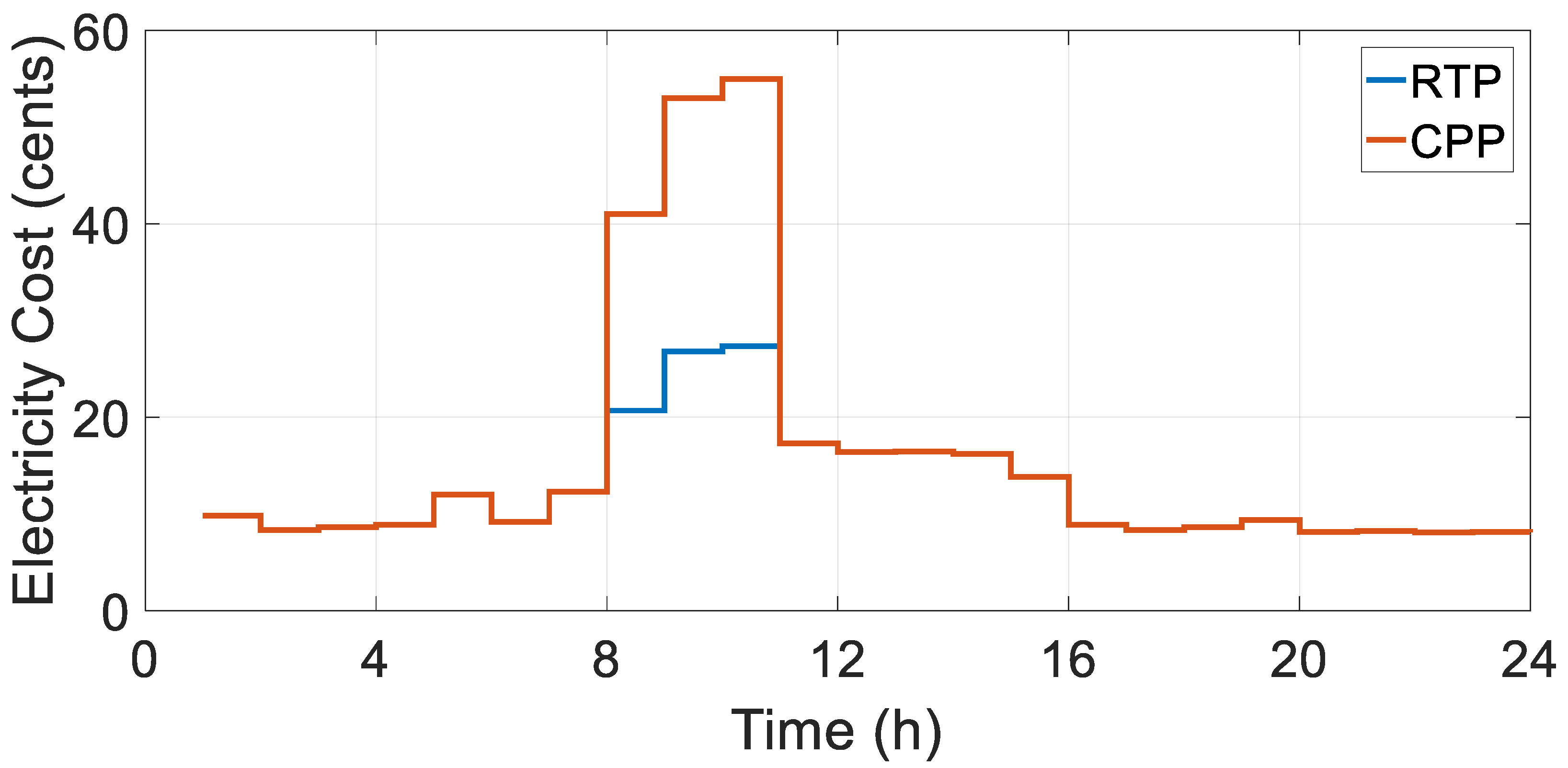
$SO{C}_{max}$	90%	$SO{C}_{min}$	30%

. Two different pricing schemes—RTP and CPP—were considered in this study. Both schemes had the same prices of energy except from 08:00 to 11:00, where the CPP scheme charged more than RTP. The peak price in both schemes was observed between 10:00 to 11:00, as shown in Figure 6. Furthermore, it was assumed that the tariff for the H2G energy export was half of the pricing charged in the energy import from the G2H [27]. Three different scenarios considering PV generation, the ESS (battery), and grid supply were analyzed in this study. The details considered regarding these scenarios are given in

Table 6. Different Scenarios.

Scenarios	Utility	Battery	PV	H2G Export
1	Yes	No	No	No
2	Yes	Yes	No	No
3	Yes	Yes	Yes	Yes

. These scenarios depict the impact of the optimal appliance scheduling on the operating cost of the electricity by considering the absence and presence of PV or/and an ESS.

7. Simulations and Results

The simulation results and discussions are presented in this section to evaluate the performance of a DSM in the presence of utility, ESS, and PV units. The three different scenarios given in Table 6 have been simulated in the MATLAB version R2016a environment using a seventh generation Intel core m3-7Y30 with a processor @ 1.61 GHz and 8 GB RAM. To tackle with the sub-optimality issue of heuristic techniques, the optimal scheduling problem was solved by running the simulation 50 times for each algorithm. All the results presented in the following subsections are the average cost calculated based on the 50 runs. The results of the proposed HGWGA in all three scenarios were compared with the two different heuristic algorithms (GA and GWO) to validate the effectiveness and better performance of the proposed algorithm. All algorithms used in this paper considered the residential load for the optimal appliance scheduling in the presence of utility, ESS, and PV units. The proposed algorithm was also compared with the unscheduled case where an EMC and SMSU were not installed.

7.1. Scenario 1: HEMS with Grid Only

In this scenario, a conventional home without an ESS or PV integration was considered. The electricity consumers of such conventional homes do not have their own ESS and PV generation. Therefore, such consumers can only import energy from the grid to fulfill their daily load requirements without any provision for H2G energy export.

7.1.1. Cost using the RTP and CPP

In the unscheduled case, the appliances completed their operations according to consumer preferences by blindly importing electricity from the utility without considering the electricity purchase tariffs. In this case, the peak load occurred from 10:00 to 11:00 when both the RTP and CPP tariffs of energy purchase were at a maximum, as shown in Figure 7. Therefore, the overall cost of the electricity consumption was increased in this case. However, in the scheduled case, when the GWO, GA, and the proposed HGWGA optimally scheduled the consumer loads by considering the RTP scheme, the costs were 474.06 cents, 462.67 cents, and 449.35 cents, respectively. In comparison with the unscheduled case, the optimal scheduling cost using the GWO, GA, and the proposed HGWGA was reduced by 10.25%, 12.41%, and 14.93%, respectively. Similarly, when the CPP signal was used, the respective electricity consumption costs were 541.45 cents, 523.96 cents, and 508.35 cents, which showed that the electricity consumption costs were reduced by 20.28%, 22.85%, and 25.15%, respectively, as shown in

Table 7. Results comparison table. AWT: appliance waiting time.

Technique Name (Case)	Electricity Cost/Day Using RTP Signal (Cents)	Electricity Cost Reduction/Day Using RTP Signal (%)	Electricity Cost/Day Using CPP Signal (Cents)	Electricity Cost Reduction/day Using CPP Signal (%)	PAR	PAR Reduction (%)	AWT (h)
Unscheduled Case	528.19	------	679.17	------	4.440	------	------
GA (Scheduled)	462.67	12.41	523.96	22.85	3.629	18.25	1.65
GWO (Scheduled)	474.06	10.25	541.45	20.28	3.774	15	1.54
Proposed HGWGA (Scheduled)	449.35	14.93	508.35	25.15	3.108	30	1.72
GA (Scheduled + ESS)	410.07	22.36	435.57	35.87	3.580	19.38	1.58
GWO (Scheduled + ESS)	422.42	20.03	432.30	36.35	3.413	23.13	1.47
Proposed HGWGA (Scheduled + ESS)	399.34	24.39	409.36	39.73	3.052	31.25	1.64
GA (Scheduled + ESS+PV)	315.61	40.25	268.79	60.42	3.588	19.18	1.55
GWO (Scheduled + ESS+ PV)	322.65	38.91	296.36	56.37	3.369	24.13	1.44
Proposed HGWGA (Scheduled + ESS + PV)	299.95	43.22	255.04	62.45	2.730	38.50	1.61

. The total electricity consumption cost for the unscheduled and scheduled cases for scenario 1 using the RTP and CPP signals is presented in Figure 8 and Figure 9, respectively.

7.1.2. PAR Using RTP and CPP

In the proposed architecture of the HEMS, an EMC and SMSU were used. Using these units, all appliances were optimally controlled in a way to avoid peaks. Therefore, the PAR in the optimally scheduled cases was reduced with respect to the unscheduled case. Both for the RTP and CPP tariffs, the PAR for the unscheduled, GA, GWO, and our proposed HGWGA was observed to be 4.44, 3.629, 3.774, and 3.108, respectively. The GA, GWO, and the proposed HGWGA diminished the PAR as compared to the unscheduled case by 18.25%, 15%, and 30%, respectively, as presented in Table 7. The PAR of the unscheduled load and scheduled load of this scenario is shown in Figure 10.

7.1.3. AWT Using RTP and CPP

In the optimal scheduling problem, the consumption cost and appliance waiting time are the two quantities among which a trade-off exists. In this scenario, the AWT for GA, GWO, and the proposed HGWGA was found to be 1.65 h, 1.543 h, and 1.72 h, respectively. It can be observed that HGWGA had the maximum AWT compared with the other implemented optimization techniques, which meant that the consumers were bound to sacrifice their comfort to achieve the cost-minimization objective. The AWT of scenario 1 for the GA, GWO, and HGWGA is presented in Figure 11.

Keeping in mind the different results for scenario 1, the percentage reduction in cost and PAR for both the RTP and CPP tariffs displays the effectiveness of the proposed hybrid technique (HGWGA) as it gives improved results in comparison with the unscheduled and other scheduled cases (GA, GWO).

7.2. Scenario 2: HEMS with an ESS

In scenario 2, the electricity consumers had their own ESS in conjunction with the grid supply to fulfill their load requirements without any RERs. In off-peak hours, the consumers stored the energy from grid in their installed ESS. In each time slot, when the dischargeable energy of the ESS was less than the consumer demand, the consumers imported energy from the grid to fulfill their load requirements. On the other hand, when the dischargeable energy of the ESS was greater than the consumer load demand, the consumers neither purchased energy from the grid nor sold their excess energy to the grid. The hourly loads of this scenario are presented in Figure 12.

7.2.1. Cost Using RTP and CPP

After obtaining the optimal scheduling through the GWO, GA, and the proposed technique HGWGA by considering the RTP tariff, the electricity consumption charges were 422.42 cents, 410.07 cents, and 399.34 cents, respectively, i.e., the optimal scheduling cost using the GWO, GA, and the proposed HGWGA was reduced by 20.03%, 22.36%, and 24.39%, respectively, in comparison with the unscheduled case. Similarly, when the CPP signal was applied, the electricity consumption costs for the GWO, GA, and the proposed technique HGWGA were 432.30 cents, 435.57 cents, and 409.36 cents, respectively, which demonstrated that consumption cost of the unscheduled case was reduced by 36.35%, 35.87%, and 39.73%, respectively, as shown in Table 7. The total electricity consumption costs for the unscheduled and scheduled cases in the RTP and CPP schemes are depicted in Figure 13 and Figure 14, respectively.

7.2.2. PAR Using RTP and CPP

When the ESS was incorporated into the proposed architecture, a greater reduction in the PAR was observed since the ESS supplied the stored energy to meet the load demand. In the unscheduled case, the PAR was 4.4 which became 3.580, 3.413, and 3.052 using optimal scheduling with the GA, GWO, and HGWGA, respectively. The percentage reduction in the PAR after the optimal scheduling using the GA, GWO, and HGWGA was 19.38%, 23.13%, and 31.25%, respectively, relative to the unscheduled case. The same PAR values were observed in both the RTP and CPP tariff schemes. The values of the PAR for the unscheduled and scheduled cases are shown in Figure 15.

7.2.3. AWT Using RTP and CPP

In scenario 2, the AWT for the GA, GWO, and HGWGA was computed to be 1.58 h, 1.47 h, and 1.64 h, respectively, which shows that there was a trade-off between the consumer consumption cost and consumer comfort. Figure 16 represents the AWT of the appliance scheduling using the optimization algorithms GA, GWO, and HGWGA.

Keeping in mind the percentage reduction in cost and PAR for scenario 2 via the GA, GWO, and HGWGA with both the RTP and CPP tariffs, the proposed hybrid technique (HGWGA) seems more promising as it gave improved results in comparison with the unscheduled and other scheduled cases obtained using the GA and GWO.

7.3. Scenario 3: HEMS with ESS and PV

In this scenario, the electricity consumer had their own ESS and a PV generation system integrated with it. The consumers fulfilled their load demand by getting energy from the PV generation, ESS, and utility. In each time interval, when the output energy of the PV plus ESS discharge energy was less than to the consumer load demand, the consumer imported energy from the utility, and whenever the output energy of PV plus ESS discharge energy was greater than the consumer load demand, then the consumer exported the extra energy to the utility at 50% of the purchasing electricity cost for both the RTP and CPP tariff schemes. In time slots 7, 8, and 11 to 18, the consumers had extra energy. Therefore, they exported their extra energy to the grid. Due to this, the total cost of the electricity consumption reduced, and the consumer got the benefits of net metering. The hourly load of this scenario is demonstrated in Figure 17.

7.3.1. Cost Using RTP and CPP

By considering the RTP tariff, the GWO, GA, and the proposed technique HGWGA optimally scheduled the consumer load in the presence of an ESS and PV, and the electricity consumption costs were 322.65 cents, 315.61 cents, and 299.95 cents, respectively. In comparison with the unscheduled case, the optimal scheduling cost using the GWO, GA, and the proposed HGWGA was reduced by 38.91%, 40.25%, and 43.22%, respectively. Similarly, when the CPP signal was applied, the respective electricity consumption costs were 296.36 cents, 268.79 cents, and 255.04 cents, which indicates that the consumption cost relative to the unscheduled case was reduced by 56.37%, 60.42%, and 62.45%, respectively. The total electricity consumption cost for the unscheduled and scheduled cases for scenario 3 using the RTP and CPP schemes is shown in Figure 18 and Figure 19, respectively.

7.3.2. PAR Using RTP and CPP

In the proposed architecture of the HEMS, an SMSU and EMC were used. Using these units, all the appliances connected to the ESS and PV were optimally controlled in a way to avoid peaks. Therefore, the PAR in the scheduled cases was reduced compared to the unscheduled case. Both for the RTP and CPP tariffs, the PAR for the unscheduled, GA, GWO, and our proposed HGWGA was found to be 4.44, 3.588, 3.369, and 2.730, respectively. The GA, GWO, and our proposed HGWGA reduced the PAR compared to the unscheduled case by 19.18%, 24.13%, and 38.5%, respectively, for both the RTP and CPP signals. Figure 20 presents the PAR value of the unscheduled and scheduled cases.

7.3.3. AWT Using RTP and CPP

In present scenario, the AWT for the GA, GWO, and HGWGA was found to be 1.55 h, 1.44 h, and 1.61 h, respectively. It can be clearly observed that HGWGA had the maximum waiting time compared with other implemented optimization techniques, which means that the consumers were bound to sacrifice their comfort to achieve the cost-minimization objective. The AWT for the GA, GWO, and HGWGA is shown in Figure 21.

The percentage reduction in the consumption cost and the PAR for both the RTP and CPP tariffs displays the effectiveness of the proposed hybrid technique (HGWGA) as it gave better results compared to the unscheduled and scheduled load techniques using the GA and GWO.

7.4. Comparison of the Execution Time

To compare the execution time of the GA, GWO, and HGWGA, each of them was run 50 times to find the solution of the scheduling problem, as discussed in Section 4. Different statistics of execution time for different cases using the RTP tariff scheme are shown in

Table 8. Comparison of the execution time of different algorithms for 50 runs.

Technique (Case)	Maximum Execution Time (s)	Minimum Execution Time (s)	Average Execution Time (s)	Standard Deviation	Variance
GA (Scheduled)	23.73	20.09	21.87	0.425	0.180
GWO (Scheduled)	21.69	16.97	18.16	0.373	0.139
Proposed HGWGA (Scheduled)	17.46	12.53	13.99	0.221	0.049
GA (Scheduled + ESS)	25.57	21.37	23.43	0.498	0.248
GWO (Scheduled + ESS)	23.19	18.29	20.65	0.407	0.165
Proposed HGWGA (Scheduled + ESS)	18.93	13.74	15.25	0.369	0.136
GA (Scheduled + ESS + PV)	28.15	22.07	23.65	0.596	0.355
GWO (Scheduled + ESS + PV)	26.27	18.47	20.42	0.515	0.265
Proposed HGWGA (Scheduled + ESS + PV)	20.59	14.83	16.09	0.493	0.241

. For all cases, it can be observed that the proposed HGWGA technique required the lowest average execution time for 50 runs to attain the optimal solution compared to the GA and GWO. In addition, as the complexity of the case study increased due to the addition of more system elements, such as PV and an ESS, the execution time required for the simulation also increased irrespective of the algorithm used. From Table 8, it is also evident that the proposed HGWGA was the more time-efficient technique among those used in this study.

The standard deviation can be a good indicator to assess the performance of an optimization algorithm for its consistent optimal solutions. In terms of execution time, the standard deviation was calculated along with its maximum and minimum values, and the results are presented in Table 8. It can be noted that the standard deviation in execution time of the proposed HGWGA was better for all cases in comparison with the GA and GWO, which validates the performance of the proposed technique.

8. Conclusions

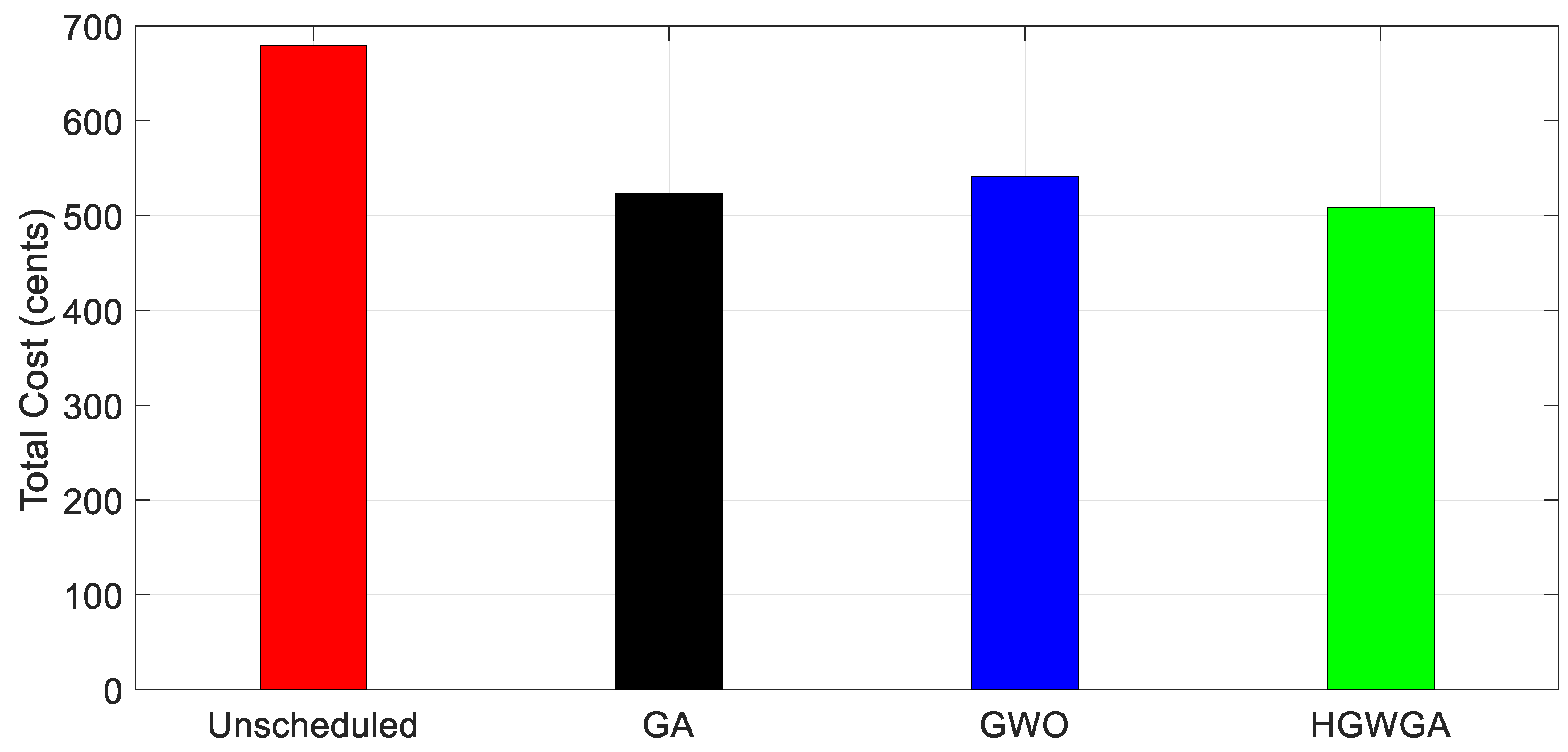
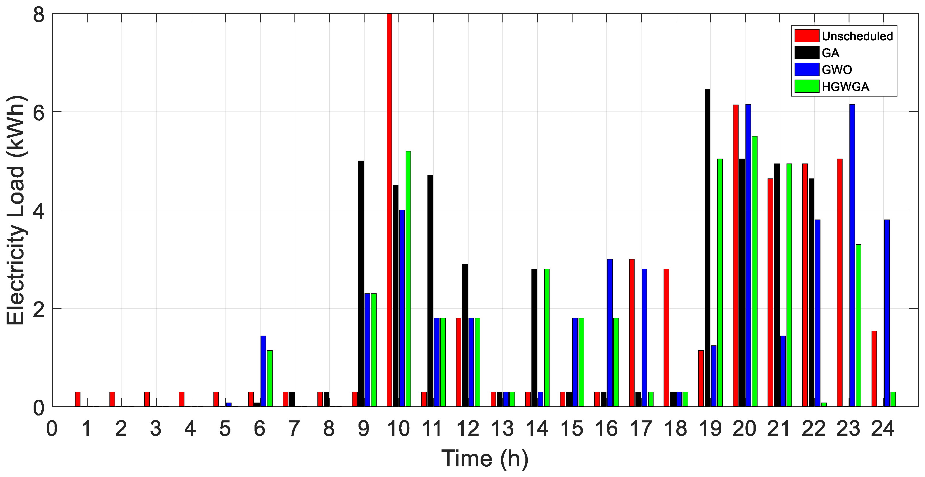
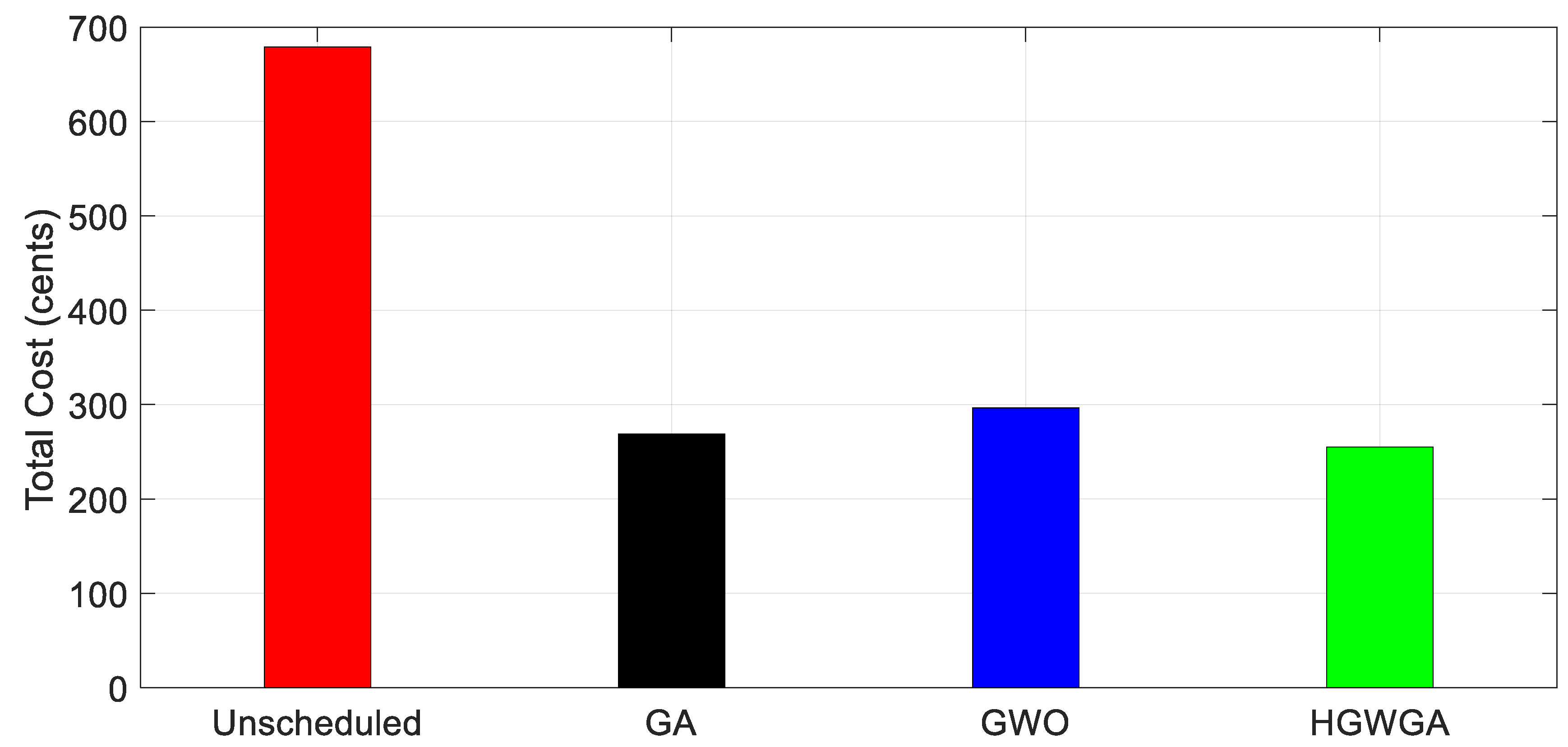
In this paper, a HEMS model was proposed for residential electricity consumers using multiple appliances with an ESS and PV generation including the option of a H2G energy exchange. A new optimization technique called HGWGA was proposed and implemented to solve the residential consumer appliance scheduling problem in the presence of an ESS and PV. The proposed hybrid algorithm was developed by combining the attributes of GWO and the GA to reduce the consumer electricity consumption cost and the PAR while considering RTP and CPP tariff schemes. To substantiate the performance, the strength and effectiveness of the proposed technique, three scenarios were considered, and the obtained results were compared with GWO, the GA, and unscheduled cases. From Table 7, it is clear that for all three scenarios, the total electricity consumption cost was reduced by 14.93%, 24.39%, and 43.22%, respectively, through the optimal appliance scheduling using the proposed HGWGA in case of just the RTP signal being present. Similarly, when the CPP signal was incorporated, the electricity consumption cost decreased by 25.15%, 39.73%, and 62.45%, and the PAR was reduced by 30%, 31.25%, and 38.5%, respectively. For all three scenarios, the percentage reduction in cost and the PAR for both the RTP and CPP tariffs displayed the effectiveness of the proposed hybrid technique. The results of the execution time demonstrated that the convergence rate of the proposed HGWGA for the scheduling of appliances was comparatively fast, and therefore, this technique can be a better choice in real-time applications in SMSUs for load scheduling.

The proposed algorithm for the optimal appliance scheduling strategy can be applied to actual data when and where they are provided. It not only reduced the energy cost, but also increased the stability and reliability of the grid. In addition, the contribution of scheduling results for several HEMSs can be important for an aggregator to manage its resources for a cost-effective and reliable operation of a microgrid.

This work focused on residential loads; however, an increase in the number of appliances and the incorporation of loads of other energy sectors, i.e., industrial and commercial, is planned for future work. In future, RERs including PV, wind, biogas, etc., will be integrated with the conventional energy generation resources to develop a hybrid energy generation system. Battery electric vehicles (BEV) and plug-in hybrid electric vehicles (PHEV) will be considered for the ESS. To improve the performance of the proposed methodology and to diminish the effects of uncertainties, stochastic models of DR strategies can be used. A hybrid of the proposed heuristic technique and fuzzy techniques can be used to further enhance the performance in the future.

References

1. Fuselli, D.; de Angelis, F.; Boaro, M.; Squartini, S. Action dependent heuristic dynamic programming for home energy resource scheduling. Int. J. Electr. Power Energy Syst. 2013, 48, 148–160. [Google Scholar] [CrossRef]
2. Mhanna, S.; Chapman, A.C.; Verbic, G. A Fast Distributed Algorithm for Large-Scale Demand Response Aggregation. IEEE Trans. Smart Grid 2016, 7, 2094–2107. [Google Scholar] [CrossRef]
3. Tükenmez, M.; Demireli, E. Renewable energy policy in Turkey with the new legal regulations. Renew. Energy 2012, 39, 1–9. [Google Scholar] [CrossRef]
4. Farhangi, H. The Path of the Smart Grid. IEEE Power Energy Mag. 2010, 8, 18–28. [Google Scholar] [CrossRef]
5. Fang, X.; Misra, S.; Xue, G.; Yang, D. Smart Grid—The New and Improved Power Grid. IEEE Commun. Surv. Tutor. 2012, 14, 944–980. [Google Scholar] [CrossRef]
6. Lior, N. Sustainable energy development: The present (2011) situation and possible paths to the future. Energy 2012, 43, 174–191. [Google Scholar] [CrossRef]
7. Erdinc, O.; Paterakis, N.G. Smart Household Operation Considering Bi-Directional EV and ESS Utilization by Real-Time Pricing-Based DR. IEEE Trans. Smart Grid 2015, 6, 1281–1291. [Google Scholar] [CrossRef]
8. Tascikaraoglu, A.; Boynuegri, A.R.; Uzunoglu, M. A demand side management strategy based on forecasting of residential renewable sources: A smart home system in Turkey. Energy Build. 2014, 80, 309–320. [Google Scholar] [CrossRef]
9. Albadi, M.H.; El-Saadany, E.F. A summary of demand response in electricity markets. Electr. Power Syst. Res. 2008, 78, 1989–1996. [Google Scholar] [CrossRef]
10. Zhao, Z.; Lee, W.C.; Shin, Y. An Optimal Power Scheduling Method for Demand Response in Home Energy Management System. IEEE Trans. Smart Grid 2013, 4, 1391–1400. [Google Scholar] [CrossRef]
11. Khalid, A.; Javaid, N.; Mateen, A. Demand Side Management using Hybrid Bacterial Foraging and Genetic Algorithm Optimization Techniques. In Proceedings of the 10th International Conference on Complex, Intelligent, and Software Intensive Systems (CISIS), Fukuoka, Japan, 6–8 July 2016; pp. 494–502. [Google Scholar]
12. Pipattanasomporn, M.; Kuzlu, M.; Rahman, S. An Algorithm for Intelligent Home Energy Management and Demand Response Analysis. IEEE Trans. Smart Grid 2012, 3, 2166–2173. [Google Scholar] [CrossRef]
13. Avci, M.; Erkoc, M.; Rahmani, A.; Asfour, S. Model predictive HVAC load control in buildings using real-time electricity pricing. Energy Build. 2013, 60, 199–209. [Google Scholar] [CrossRef]
14. Yang, J.; Zhang, G.; Ma, K. Matching supply with demand: A power control and real time pricing approach. Int. J. Electr. Power Energy Syst. 2014, 61, 111–117. [Google Scholar] [CrossRef]
15. Manzano-agugliaro, F.; Montoya, F.G.; Gil, C.A. Alcayde, J. Gómez, and R. Ba, Optimization methods applied to renewable and sustainable energy: A review. Renew. Sustain. Energy Rev. 2011, 15, 1753–1766. [Google Scholar]
16. Shareef, H.; Ahmed, M.S.; Mohamed, A.; al Hassan, E. Review on Home Energy Management System Considering Demand Responses, Smart Technologies, and Intelligent Controllers. IEEE Access 2018, 6, 24498–24509. [Google Scholar] [CrossRef]
17. Zhang, D.; Evangelisti, S.; Lettieri, P.; Papageorgiou, L.G. Economic and environmental scheduling of smart homes with microgrid: DER operation and electrical tasks. Energy Convers. Manag. 2016, 110, 113–124. [Google Scholar] [CrossRef]
18. Bradac, Z.; Kaczmarczyk, V.; Fiedler, P. Optimal Scheduling of Domestic Appliances via MILP. Energies 2015, 8, 217–232. [Google Scholar] [CrossRef]
19. Huang, G.; Yang, J.; Wei, C. Cost-Effective and comfort-aware electricity scheduling for home energy management system. In Proceedings of the IEEE International Conference on Big Data and Cloud Computing, Atlanta, GA, USA, 8–10 October 2016; pp. 453–460. [Google Scholar]
20. Lokeshgupta, B.; Sivasubramani, S. Multi-objective home energy management with battery energy storage systems. Sustain. Cities Soc. 2019, 47, 1–13. [Google Scholar]
21. Kuzlu, M. Score-based intelligent home energy management (HEM) algorithm for demand response applications and impact of HEM operation on customer comfort. IET Gener. Transm. Distrib. 2015, 9, 627–635. [Google Scholar] [CrossRef]
22. Mohamed, F.A.; Koivo, H.N. Online management genetic algorithms of microgrid for residential application. Energy Convers. Manag. 2012, 64, 562–568. [Google Scholar] [CrossRef]
23. Javaid, N.; Javaid, S.; Abdul, W.; Ahmed, I. A Hybrid Genetic Wind Driven Heuristic Optimization Algorithm for Demand Side Management in Smart Grid. Energies 2017, 10, 319. [Google Scholar] [CrossRef]
24. Abid, M.M.N.; Javaid, N.; Rahim, M.H. Demand side management for residential areas using hybrid bacterial foraging and bat optimization algorithm. In Proceedings of the IEEE International Conference on Computing, Mathematics and Engineering Technologies (iCoMET), Sukkur, Pakistan, 3–4 March 2018; pp. 1–8. [Google Scholar]
25. Mahmood, A.; Javaid, N.; Khan, N.A.; Razzaq, S. An optimized approach for home appliances scheduling in smart grid. In Proceedings of the IEEE 19th International Multi-Topic Conference (INMIC), Islamabad, Pakistan, 5–6 December 2016; pp. 1–5. [Google Scholar]
26. Rehman, N.; Rahim, H.; Ahmad, A.; Khan, Z.A.; Qasim, U.; Javaid, N. Heuristic Algorithm based Energy Management System in Smart Grid. In Proceedings of the IEEE 10th International Conference on Complex, Intelligent, and Software Intensive Systems (CISIS), Fukuoka, Japan, 6–8 July 2016; pp. 396–402. [Google Scholar]
27. Yang, J.; Liu, J.; Fang, Z.; Liu, W. Electricity scheduling strategy for home energy management system with renewable energy and battery storage: A case study. IET Gener. Transm. Distrib. 2018, 12, 639–648. [Google Scholar] [CrossRef]
28. Liao, J.T.; Yang, H.T. Novel Electron Drifting Algorithm Based BESS Scheduling in Home Energy Management System. In Proceedings of the IECON 2016-42nd Annual Conf. of the IEEE Industrial Electronics Society, Florence, Italy, 23–26 October 2016; pp. 3996–4001. [Google Scholar]
29. Javaid, N.; Ullah, I.; Akbar, M.; Iqbal, Z.; Khan, F.A. An Intelligent Load Management System with Renewable Energy Integration for Smart Homes. IEEE Access 2017, 5, 13587–13600. [Google Scholar] [CrossRef]
30. Basit, A.; Ahmad, G.; Sidhu, S.; Mahmood, A. Efficient and Autonomous Energy Management Techniques for the Future Smart Homes. IEEE Trans. Smart Grid 2017, 8, 917–926. [Google Scholar] [CrossRef]
31. Mary, G.A.; Rajarajeswari, R. Smart Grid Cost Optimization using Genetic Algorithm. Int. J. Res. Eng. Technol. 2014, 3, 282–287. [Google Scholar]
32. Bharathi, C.; Vijayakumar, V. Genetic Algorithm Based Demand Side Management for Smart Grid. Wirel. Pers. Commun. 2017, 93, 481–502. [Google Scholar] [CrossRef]
33. Asgher, U.; Rasheed, M.B.; Al-Sumaiti, A.; Rahman, A.U.; Ali, I.; Alzaidi, A.; Alamri, A. Smart energy optimization using heuristic algorithm in smart grid with integration of solar energy sources. Energies 2018, 11, 3494. [Google Scholar] [CrossRef]
34. Sharifi, A.H.; Maghouli, P. Energy management of smart homes equipped with energy storage systems considering the PAR index based on real-time pricing. Sustain. Cities Soc. 2019, 45, 579–587. [Google Scholar] [CrossRef]
35. Aslam, S.; Iqbal, Z.; Javaid, N.; Khan, Z.A.; Aurangzeb, K.; Haider, S.I. Towards efficient energy management of smart buildings exploiting heuristic optimization with real time and critical peak pricing schemes. Energies 2017, 10, 2065. [Google Scholar] [CrossRef]
36. Hafeez, G.; Javaid, N.; Iqbal, S.; Khan, F.A. Optimal residential load scheduling under utility and rooftop photovoltaic units. Energies 2018, 11, 611. [Google Scholar] [CrossRef]
37. Tsui, K.M.; Chan, S.C. Demand Response Optimization for Smart Home Scheduling Under Real-Time Pricing. IEEE Trans. Smart Grid 2012, 3, 1812–1821. [Google Scholar] [CrossRef]
38. Wu, Z.; Zhou, S.; Li, J. Real-time scheduling of residential appliances via conditional risk-at-value. IEEE Trans. Smart Grid 2014, 5, 1282–1291. [Google Scholar] [CrossRef]
39. Naz, M.; Iqbal, Q.Z.; Javaid, N.; Khan, Z.A.; Abdul, W.; Al-Mogren, A.s.; Alamri, A. Efficient power scheduling in smart homes using hybrid grey Wolf differential evolution optimization technique with real time and critical peak pricing schemes. Energies 2018, 11, 384. [Google Scholar] [CrossRef]
40. Khan, Z.A.; Zafar, A.; Javaid, S.; Aslam, S.; Rahim, M.H.; Javaid, N. Hybrid meta-heuristic optimization based home energy management system in smart grid. J. Ambient Intell. Humaniz. Comput. 2019, 1, 1–17. [Google Scholar] [CrossRef]
41. Setlhaolo, D.; Xia, X.; Zhang, J. Optimal scheduling of household appliances for demand response. Electr. Power Syst. Res. 2014, 116, 24–28. [Google Scholar] [CrossRef]
42. Zhu, Z.; Tang, J.; Lambotharan, S.; Chin, W.H.; Fan, Z. An Integer Linear Programming Based Optimization for Home Demand-side Management in Smart Grid. In Proceedings of the IEEE PES Innovative Smart Grid Technologies (ISGT), Perth, Australia, 13–16 November 2011; pp. 1–5. [Google Scholar]
43. Samadi, P.; Member, S.; Wong, V.W.S.; Member, S.; Schober, R. Load Scheduling and Power Trading in Systems With High Penetration of Renewable Energy Resources. IEEE Trans. Smart Grid 2016, 7, 1802–1812. [Google Scholar] [CrossRef]
44. Khan, M.F.N.; Malik, T.N. Probablistic generation model for optimal allocation of PV DG in distribution system with time-varying load models. J. Renew. Sustain. Energy 2017, 9, 1–21. [Google Scholar] [CrossRef]
45. Khan, M.F.N.; Malik, T.N.; Sajjad, I.A. Impact of time varying load models on PV DG planning. J. Renew. Sustain. Energy 2018, 10, 1–21. [Google Scholar]
46. Sajjad, I.A.; Manganelli, M.; Martirano, L.; Chicco, G.; Parise, G. Net Metering Benefits for Residential Buildings: A Case Study in Italy. In Proceedings of the IEEE 15th International Conference on Environment and Electrical Engineering (ICEEE), Rome, Italy, 10–13 June 2015; pp. 1–6. [Google Scholar]
47. Muralitharan, K.; Sakthivel, R.; Shi, Y. Multiobjective optimization technique for demand side management with load balancing approach in smart grid. Neurocomputing 2016, 177, 110–119. [Google Scholar] [CrossRef]
48. Holland, J. Adaptation in Natural and Artificial Systems; University Michigan: Ann Arbor, MI, USA, 1975. [Google Scholar]
49. de Jong, K. An Analysis of the Behavior of a Class of Genetic Adaptive Systems; Dr. Diss. Ann Arbor Univ. Michigan: Ann Arbor, MI, USA, 1975. [Google Scholar]
50. Goldberg, D.E. Genetic Algorithms in Search, Optimization, and Machine Learning; Addison-Wesley Longman Publishing Co., Inc.: Boston, MA, USA, 1989; pp. 1–432. [Google Scholar]
51. Beasley, R.M.D.; Bull, D.R. An Overview of Genetic Algorithms: Part 1, Fundamentals. Univ. Comput. 1993, 15, 58–69. [Google Scholar]
52. Mirjalili, S.; Mohammad, S.; Lewis, A. Advances in Engineering Software Grey Wolf Optimizer. Adv. Eng. Softw. 2014, 69, 46–61. [Google Scholar] [CrossRef] [Green Version]
53. Iqbal, Z.; Javaid, N.; Iqbal, S.; Aslam, S.; Khan, Z.A. A domestic microgrid with optimized home energy management system. Energies 2018, 11, 1002. [Google Scholar] [CrossRef] [Green Version]
Figure 1. Classification of demand response (DR) programs.
Applsci 09 05226 g001
Figure 2. Proposed system model. AMI: advanced metering infrastructure, EMC: energy management controller, ESS: energy storage system, PV: photovoltaic, SMSU: smart scheduler unit.
Applsci 09 05226 g002
Figure 3. Status of the appliances’ execution pattern.
Applsci 09 05226 g003
Figure 4. Flowchart of the proposed hybrid grey wolf genetic algorithm (HGWGA) technique.
Applsci 09 05226 g004
Figure 5. Solar irradiance patterns: (a) original solar irradiance patterns and (b) solar irradiance patterns generated using the beta distribution.
Applsci 09 05226 g005
Figure 6. Price data.
Applsci 09 05226 g006
Figure 7. Per-hour load without an energy storage system (ESS) or photovoltaics (PV).
Applsci 09 05226 g007
Figure 8. Total cost using the real-time pricing (RTP).
Applsci 09 05226 g008
Figure 9. Total cost using the critical peak pricing (CPP).
Applsci 09 05226 g009
Figure 10. Peak-to-average ratio (PAR) without an ESS or PV.
Applsci 09 05226 g010
Figure 11. AWT without ESS or PV.
Applsci 09 05226 g011
Figure 12. Per-hour load with ESS.
Applsci 09 05226 g012
Figure 13. Total cost with an ESS using the RTP.
Applsci 09 05226 g013
Figure 14. Total cost with an ESS using the CPP.
Applsci 09 05226 g014
Figure 15. PAR with an ESS.
Applsci 09 05226 g015
Figure 16. AWT with ESS.
Applsci 09 05226 g016
Figure 17. Per-hour load with an ESS and PV.
Applsci 09 05226 g017
Figure 18. Total cost with an ESS and PV using the RTP.
Applsci 09 05226 g018
Figure 19. Total cost with an ESS and PV using the CPP.
Applsci 09 05226 g019
Figure 20. PAR with an ESS and PV.
Applsci 09 05226 g020
Figure 21. AWT with an ESS and PV.
Applsci 09 05226 g021