1. Introduction
Salvage of floating objects is an important part of water source conservation. At present, interception and manual salvage are the main methods for the salvage task [
1]. These methods are labor consuming and dangerous. Although manipulating robots overcomes the shortcomings noted above [
2,
3], it requires skilled operators and cannot operate around the clock. With the development of image processing and computer vision, the use of autonomous salvage technology in surface cleaning robots has attracted great interest from researchers, and one of its most important elements is the fast and robust detection of floating objects. However, small sample acquisition is a tough problem due to the diversity and rarity of floating objects in different water areas. Additionally, interference factors such as ripple, reflection, and uneven illumination also make it difficult to find a general model for various complex water scenarios.
Few researchers have focused on floating object detection with respect to complex water surfaces. In general, the existing methods that can be applied to the detection task fall into four categories: traditional image segmentation, saliency detection, hand-crafted feature detection, and object detection based on a Convolutional Neural Network (CNN). According to different processing domains, these methods can also be classified into spatial-based methods and frequency-based methods.
In spatial domain, traditional image segmentation has an excellent real-time performance [
4]. Wang et al. [
5] extracted contours of floating objects according to image grayscale, then framed the contours that met a special size criterion. Xue et al. [
6] used the Super-pixel Merging method to segment eligible foreground regions. Tang et al. [
7] used Mean-shift clustering and an improved Otsu [
8] method to detect floating objects. Although these methods work well in calm water, they are not robust enough when ripples or reflections exist. To this end, Jin et al. [
9] proposed an improved Gaussian Mixture Model Based (GMM-based) automatic segmentation method (IGASM) to detect water surface floats, but it is not applicable in static images or in images with severe interferences.
Spatial-based object detection methods can be applied to floating object detection and have a certain anti-interference ability [
10,
11]. Traditional methods of combining hand-crafted features with classifiers are simple and fast [
12]. Hand-crafted texture features with grayscale invariance, e.g., Histogram of Oriented Gradient (HOG) [
13], Local Binary Pattern (LBP) [
14], and Gray Level Co-occurrence Matrix (GLCM) [
15], are suitable for describing floating objects under uneven illumination. But these features do not utilize global information, making feature descriptors inaccurate when other sever interferences exist. Therefore, it is necessary to extract very suitable features with respect to the special detection task, i.e., floating object detection in complex water scenes. Some algorithms based on CNN do not need to manually extract features and perform well in speed and accuracy, e.g., a Region-based Fully Convolutional Network (R-FCN) [
16], Single Shot Multi-Box Detector (SSD) [
17], Single Shot Refinement Detector (RefineDet) [
18], and the You Only Look Once (YOLOv3) method [
19]. However, in the case of a small sample, CNN-based methods are prone to over-fitting due to their multi-layer convolutions. To this end, saliency detection methods based on visual attention mechanism can solve the problem of small sample. But spatial-based saliency detection methods, e.g., Global Contrast-based Saliency Detection (RC) [
20], Contrast-based Filtering for Saliency Detection (SF) [
21] and Boolean Map for Saliency Detection (BMS) [
22] are generally sensitive to parameter selection, which limits their generalization in multiple scenarios.
In the frequency domain, frequency-based saliency detection methods, such as the Spectral Residual (SR) approach [
23], Frequency-tuned (FT) method [
24], and Maximum Symmetric Surround (MSS) method [
25] have fewer parameters and less time consumption than those saliency detection methods in a spatial domain. However, in the case of large ripple, reflection, and other interference factors, redundancies of salient maps are difficult to eliminate, resulting in extreme high false alarm rates.
In order to overcome the problems of small sample acquisition and several interference factors, i.e., ripple, reflection, and uneven illumination in floating objects detection, a simple but effective method combining spatial and frequency domains is proposed. In the spatial domain, after training with few positive samples, sliding image blocks are roughly classified by Support Vector Machines (SVM) [
26,
27,
28] with a Fused Histogram of Oriented Gradient (FHOG) features [
29] and GLCM features to detect floating objects. In the frequency domain, Gaussian high-pass filtering and phase spectrum reconstruction are implemented to preliminarily suppress the interferences. Then, global and local low-rank decompositions [
30,
31] are carried out to remove the residual redundant regions. Finally, bounding boxes from different processing domains are combined by analyzing Intersection-over-Unions (IoUs) to frame real objects accurately.
The main contributions of this paper are as follows:
An effective combination of hand-crafted texture features, i.e., FHOG and GLCM. The new combined features describe floating objects more accurately than traditional HOG, GLCM, and LBP features in complex water scenes, while its time consumption of feature extraction is comparable to the traditional ones.
A new anti-interference saliency detection method. The method processes a frequency spectrum and adopts low-rank matrix decomposition to accurately detect floating objects without any training samples. Note that the method effectively solves the problems caused by ripple, reflection, and uneven illumination, and performs better than other sample-free saliency detection methods.
A novel floating object detection algorithm combining spatial-based texture detection and frequency-based saliency detection. The combined algorithm is characterized by small sample training, low time consumption, strong anti-interference ability, and high precision.
The rest of this paper is organized as follows.
Section 2 introduces the methodology, including the proposed algorithm framework, detailed implementations in different processing domains, and the strategy of combination.
Section 3 presents and analyzes the comprehensive results. Parameter selections and comparative experiments are also conducted in
Section 3.
Section 4 draws the conclusion.
2. Methodology
All images applied are collected by a surface cleaning robot. One of the key tasks of the robot is to detect floating objects in different water areas. Algorithm 1 is the framework of our floating object detection algorithm for each video frame.
| Algorithm 1 Floating Object Detection |
Input: I
Output: B1, B2, B3
1: B1 ← TextureDetection(I)
2: B2 ← SaliencyDetection(I)
3: B3 ← Combination(B1, B2)
4: return B1, B2, B3 |
As shown in Algorithm 1, the input is a video frame I, and the detection task is carried out in three parts: texture detection, saliency detection, and combination. The outputs are three vectors of bounding boxes, i.e., B1, B2, and B3, which are the results of the three parts, respectively. Note that the final output B3 can be an empty vector, indicating that there are no floating objects in this video frame. More details are given in the subsections below.
2.1. Texture Detection in Spatial Domain
Currently, the state-of-the-art methods of universal object detection are usually based on the data-driven CNN. Taking the commonly used 16-depth network by Visual Geometry Group (VGG16-Net) as an example, the convolutional neural network has about 138 million parameters, so thousands of training samples are required to solve the over-fitting problem. However, due to the diversity and rarity of floating objects on different water surfaces, only hundreds or even dozens of effective source images can be collected, which makes it difficult to robustly detect floating objects with CNN-based methods. Although there are a series of Transfer Learning methods [
32,
33,
34] and Data Augmentation strategies [
35,
36] that help CNN models fit methods without plenty of source images, these training skills cannot essentially improve the detection precision and maximize the performance of CNN. Therefore, the popular CNN-based methods may not be the best choices of floating object detection in the case of small sample acquisition.
To solve the problem of over-fitting caused by insufficient training samples, we adopted Latent SVMs as the classifiers instead of convolutional neural networks. Unlike neural networks, Latent SVMs adopt the optimization goal of minimizing structural risk rather than empirical risk, and use the principle of maximum margin to reduce the requirements of data size and data distribution [
26,
27,
28]. Therefore, small sample training with SVM is able to complete a rough detection task. More importantly, SVM is insensitive to the problem of sample imbalance when all background windows are treated as negative samples. Experiments shown in
Section 3 will prove that SVM is effective enough for the rough texture detection task, and more details of SVM training are provided in the later experiment section.
In order to ensure that our classifier has a high hit rate (while high false alarm rate is acceptable at this stage), it is necessary to extract very reliable features which helps to clearly distinguish foregrounds and backgrounds. To this end, the combination of FHOG and GLCM features is adopted. The new texture features have good grayscale invariance and rotation invariance, which effectively describe global and local information of floating objects in complex water scenes.
2.1.1. FHOG Feature Extraction
The traditional HOG method firstly divides the image into many cells (e.g., size 8 × 8 pixels), and then calculates the histogram of nine unsigned gradient directions for each cell [
13]. However, this method considers two regions separated at 180 degrees to be identical, which is not accurate to describe floating objects with 360-degree rotation directions. To guarantee the ability of feature description, the HOG method extracts texture features by sliding image blocks with a small stride. Therefore, the dimension of final feature descriptor is very high, which leads to high time complexity and over-fitting, especially in the case of small sample training.
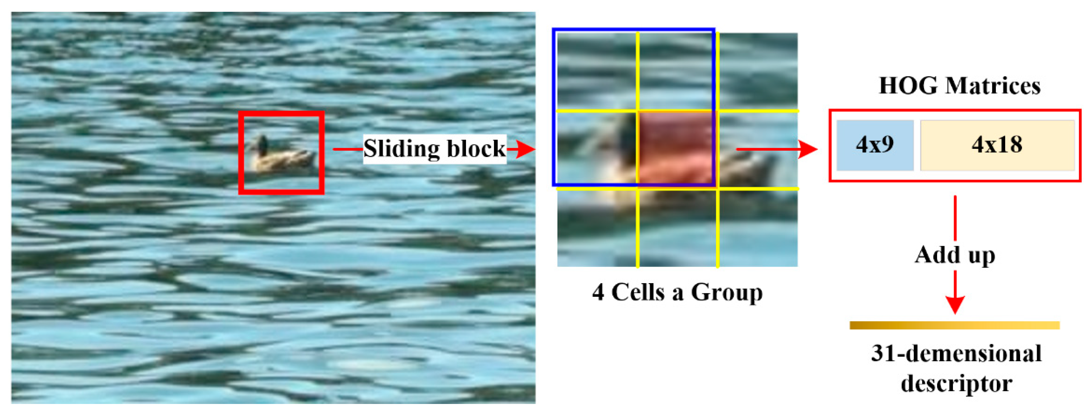
As shown in
Figure 1, an improved HOG named FHOG is adopted. First, the nine cells in a sliding image block are divided into four groups. In each group, an 18-dimensional signed HOG eigenvector and a 9-dimensional unsigned HOG eigenvector are combined into a 4 × 27 matrix. Then, columns of the matrix are added up to get a 1 × 27 vector, while rows of the matrix are added up to get a 4 × 1 vector. Finally, through connecting the two vectors, a 31-dimensional FHOG eigenvector (describing a block with nine cells) is obtained. Note that when describing the same block with nine cells, traditional HOG method needs an 81-dimensional descriptor, which is 50 dimensions larger than that of FHOG. More importantly, FHOG not only improves the speed of feature extraction, but also has a better feature description ability.
2.1.2. GLCM Feature Extraction
To further improve the ability of feature description, GLCM features are extracted. An HOG-like feature is the statistical result of pixels at different gray levels, while GLCM describes grayscale relationships between pixels and their adjacent pixels [
15]. GLCM provides information about the directions and the extents of grayscale changes, but it cannot provide the information in the form of descriptors. Therefore, statistical attributes are used to quantitatively describe texture characteristics on the basis of the GLCM matrix.
Based on the priori knowledge that textures of image blocks containing floating objects change dramatically, while textures of other background blocks change relatively gently, four statistical attributes, i.e., Energy
Eg, Entropy
Eg, Homogeneity
Ho, and Contrast
Ct are calculated. The definition is Equation (1):
where P is the probability matrix obtained by normalizing the GLCM matrix. Energy, Contrast, and Homogeneity reflect the thickness, depth, and variability of the texture, respectively, and Entropy measures the amount of information in an image. At the same time, textures of the foreground image blocks with floating objects are more delicate and more dramatic than the background blocks only with water surfaces. Therefore, the energy, uniformity, and contrast of the foregrounds are small, while the entropy values are large. Through these four attributes, foreground, and background areas can be well distinguished. Our calculation step is 2, and the directions are 0 degrees, 45 degrees, 90 degrees, and 135 degrees. Finally, a 16-dimensional descriptor can be extracted from each sliding window. Experimental results (in
Section 3) show that the combination of GLCM features and FHOG features is more conducive to detecting floating objects than traditional texture features.
2.2. Saliency Detection in Frequency Domain
A novel frequency-based saliency detection method for floating objects in complex scenes is proposed. Different from the mainstream saliency methods such as BMS [
22], the Multi-task Sparsity Pursuit method (MBP) [
37], RC [
20], MSS [
25], SR [
23], and FT [
24], our method can better solve the problems caused by waves, reflections, and uneven illumination. Algorithm 2 is the framework of our saliency detection algorithm for each video frame.
| Algorithm 2 Saliency Detection |
Input:I
Output:B2
Stage 1: Initial Saliency Map
1: G← GammaCorrection(I)
2: H← GaussianHighpassFitering(G)
3: P← PhaseReconstruction(H)
Stage 2: Redundancy Removal
4: Pg← MatrixDecomposition(P)
5: N1, N2, …, Nt← CreateBlocks(P)
6: fori = 1 → k do
7: Mi ← MatrixDecomposition(Ni)
8: Si ← ComputeNorm(Mi)
9: Ni ← Supression(Ni, Si)
10: end for
11: Pl ← Merge(N1, N2, …, Nk)
Stage 3: Ultimate Saliency Map
12: Pf ← γPg + (1 − γ)Pl
13: B2 ← BoundBox(Pf)
14: return B2 |
In saliency detection, as shown in Algorithm 2, the processing steps fall into three stages. Aiming at obtaining an initial saliency map with obvious foreground and background distinctions, the first stage includes gamma correction, Gaussian high-pass filtering, and phase spectrum reconstruction. The second stage aims to remove the scattered redundancies in the initial saliency map, and obtain the global and local saliency maps. At this stage, splitting and merging image blocks are needed for local low-rank decompositions. The third stage is to obtain the ultimate saliency map by fusing global and local saliency maps, and output the bounding box vectors as the final results.
2.2.1. Initial Saliency Map
Gamma correction (i.e., power operation on each pixel) is performed to reduce the impacts of uneven illumination, while Gaussian high-pass filtering is to suppress the ripples and reflections to some extent. The transfer function of Gaussian high-pass filter is:
where
H(
u,
v) is the transfer function of the filter,
D(
u,
v) is the distance from point (
u,
v) to the origin of the Fourier transform center, and
D0 is the cut-off frequency of the filter.
Amplitude spectrum of the image mainly contains the information of brightness, and phase spectrum mainly contains the information of texture structure [
30]. Therefore, a phase spectrum reconstruction is performed to reduce the impacts caused by ripples and uneven illumination. Then, an initial saliency map is obtained.
2.2.2. Redundancy Removal
Although most of the redundant regions have been obviously suppressed by the operations above, the scattered redundancies still need to be removed. Based on Chandrasekaran’s matrix decomposition theory [
31] that an input matrix can be decomposed into a sparse part and a low-rank part, an image can be represented as the following two parts:
where
L(
x,
y) is the low-rank part corresponding to the background, and
M(
x,
y) is the sparse noises corresponding to the salient regions. The decomposition is implemented by Equation (4):
where
P is the input matrix. This is a Non-deterministic Polynomial Hard (NP-Hard) problem, so Equation (4) is optimized by Equation (5):
where
ε is a balance coefficient, and we set
ε as 0.01. When the input matrix
P is an initial saliency map, a global saliency map
Pg = L is obtained. However, global decomposition cannot remove all of the redundancies. To this end, local decomposition is performed as follows.
First, initial saliency map is divided into k blocks of the same size (i.e.,
N1,
N2,
Nk). Next, grayscale features from all the blocks are extracted independently and combined into a matrix
Y, as shown in Equation (6):
where
yi is the column vector obtained by averaging each row of pixels in the
ith image block
Ni. Then,
Y is decomposed by Equation (5), and the saliency level
S of
Ni is obtained by Equation (7):
We have difference strategies to process the blocks according to
S, which is a key step of obtaining the local saliency map:
where
σ1 and
σ2 are the thresholds, while
μ1 and
μ2 are the suppression coefficients. Experiment results show that the best thresholds are 0.3 and 0.7, and the suppression coefficients are 0.2 and 0.8. Note that when
Si >
σ2, the block
Ni will not be processed.
2.2.3. Ultimate Saliency Map
We fuse the global and local saliency maps in a simple way:
where
γ is the weight of the global saliency map,
Pf is the ultimate saliency map, i.e., the result of saliency detection.
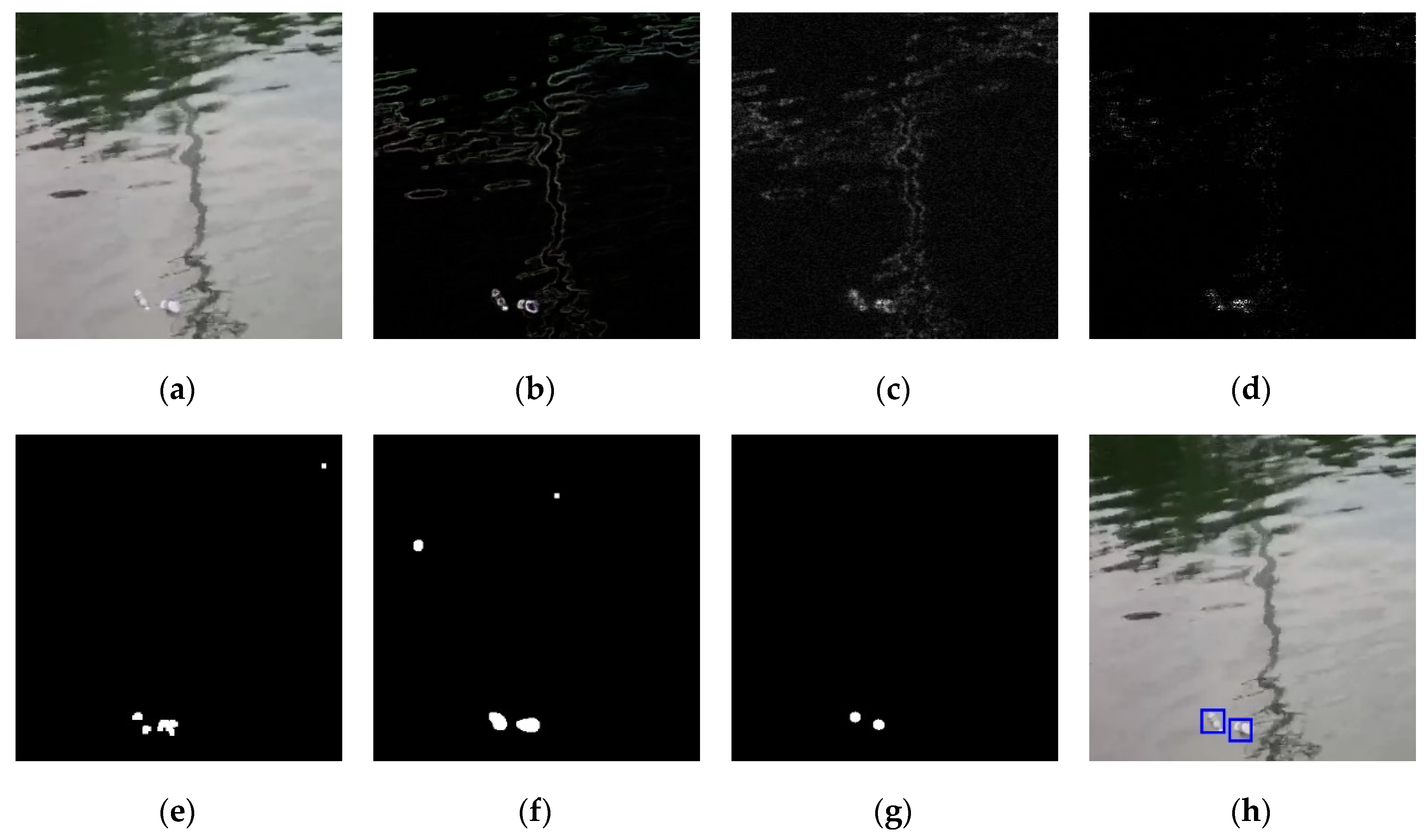
Figure 2 intuitively shows the entire process. In
Figure 2a, huge and abrupt reflections (at the top and middle of the image) make floating objects (at the bottom of the image) inconspicuous.
Figure 2b shows that gamma correction handles the illumination problem well. In
Figure 2c, most of the non-salient parts are obviously suppressed by Gaussian high-pass filtering.
Figure 2d shows that phase spectrum reconstruction makes salient regions relatively concentrated and makes redundant parts dispersed.
Figure 2e,f shows the binary images of global saliency map, local saliency map, and ultimate saliency map, respectively. Note that the method of binarization are all Otsu. In
Figure 2e,f, global or local decomposition can remove most of the redundant parts, but it is not able to remove all redundancies. However, as shown in
Figure 2g,h, through a fusing operation, the final result is much closer to the ground truth.
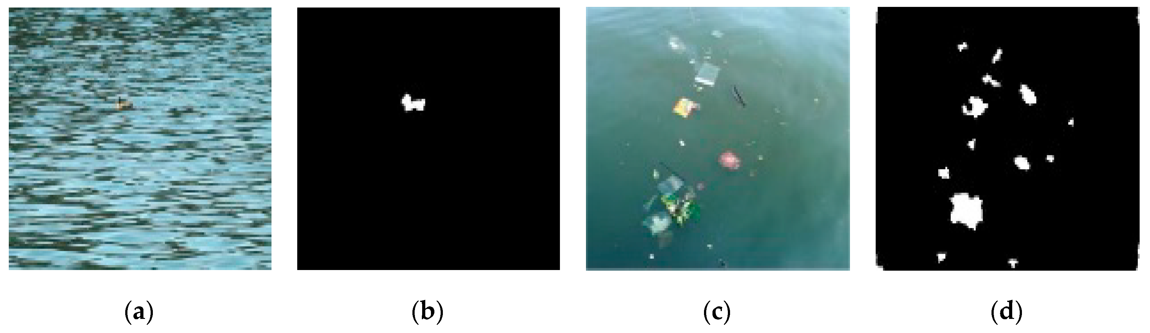
Since it is completely independent of training samples, our saliency detection method can be applied to detect any floating objects. As shown in
Figure 3, even if the floating object in the scene is indistinguishable to the naked eye, or the scene has many targets, our method can successfully detect different unknown floating objects. In
Figure 3a,b, the low contrast duck on the turbulent surface was detected. In
Figure 3c,d, multiple floating litters of different sizes on the clam surface were detected. Note that the smallest object detected in
Figure 3d is approximately 10x10 pixels in size, indicating that our saliency detection method has potential in small object detection.
2.3. Combination
Multiple candidate regions can be obtained by the above methods in spatial and frequency domains. However, these candidate regions may intersect or overlap with each other. So confirmation is needed to get the final bounding boxes, i.e.,
B3. First, Intersection-over-Unions (IoUs) of the bounding boxes from spatial and frequency domains are calculated by Equation (10):
where
A and
B are two bounding boxes from texture detection and saliency detection, respectively, and they constitute a pair of combinations. Note that in a certain video frame, there are
M ×
N similar combinations.
M and
N are the number of bounding boxes from texture detection and saliency detection, respectively. The final result from the candidates is obtained by an Intersection-over-Unions Based (IoU-based) strategy, as shown in Equation (11):
where
C is the result of combining texture detection and saliency detection;
τ1 and
τ2 are the thresholds;
R1 and
R2 are replacement rates. Experiments results show that the best thresholds are 0.2 and 0.8, respectively. The replacement rate is similar to the confidence of a bounding box, which is calculated through Equation 12:
where
R1 and
R2 are the replacement rates of the results of texture detection and saliency detection, respectively. The combination strategy not only strictly judges the existence of floating objects, but also makes the final detection result close to the ground truth.
3. Experiments
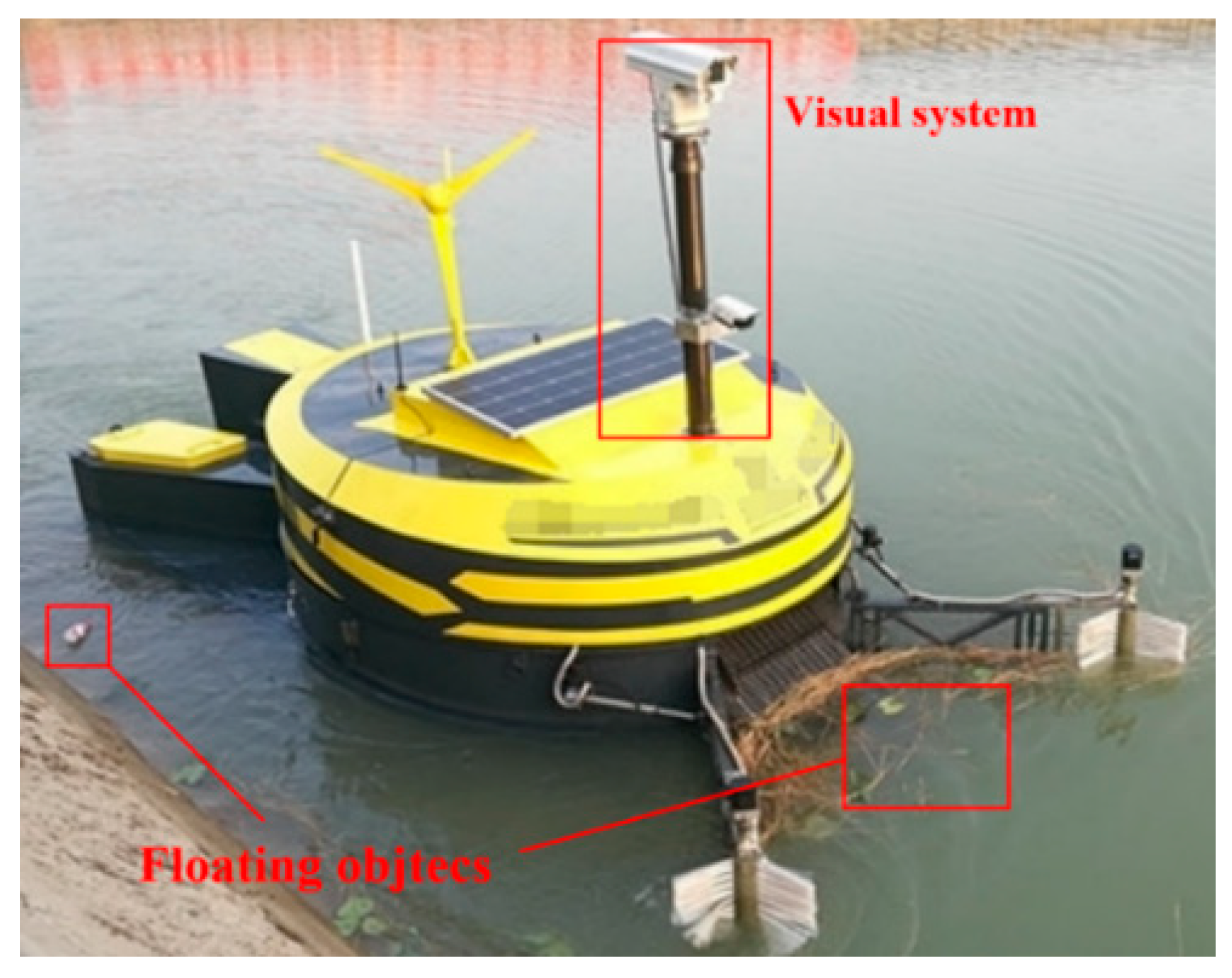
In this section, the detection results in spatial domain, frequency domain and spatial-frequency domain are firstly shown intuitively. Then, through a series of ablation experiments, the optimal parameters are given. Finally, we compare our final results with other floating object detection methods. All experiments are conducted in an unmanned surface cleaning robot shown in
Figure 4. The robot is composed of an image processing unit, a navigation unit, a conveyor caterpillar, etc. The visual system consists of two HIKVISION B12-IPOE surveillance cameras, and the CPU of the image processing unit is Intel (R) Xeon (R) E5-2660 2.20 GHz. Note that no GPU is involved in running the program. The programming libraries used are OpenCV 4.0.1 and Eigen 3.3.7.
Experimental images were sampled from 10 different water surfaces, and each area has 40 images resized into 350 × 350 pixels. Interference factors in these samples include different illumination intensities, waveform shapes, turbulence levels, reflection sizes, etc. Of these 400 source images, 280 were for training and 120 for testing, and all of them have appropriate ground truth labels. Note that in the testing set consisting of 120 source images, 140 distinct floating objects are labeled as positive samples, because some images contain multiple floating objects. Additionally, there are 10 images (1 image each water scene) without any floating objects.
3.1. Intuitive Results of Texture Detection
To intuitively compare the effects of our feature with other mainstream features (LBP [
14], HOG [
13], GLCM [
15], FHOG [
29]) in the task of floating object detection, a comparative experiment is conducted. The experiment occurred under seven challenging water scenes, including large waves, circular ripples, spray, turbulent water surface, strip ripples, near-view reflection, and far-view reflection. In this comparative experiment, the feature extraction method was the only variable, so it was necessary to keep sample generation and classification methods consistent.
Sample generation. The positive samples are not directly cropped from ground truth labels, because one of the most important features of our classification was is the dramatic change of texture features. Instead, positive samples were generated by cropping special images blocks from the 280 source images. These image blocks had the same centers of the corresponding ground truth labels, while their sizes are all 48 × 48 pixels. From each source image, negative samples were generated by cropping sliding image blocks (48 × 48 pixels in size and 20 pixels in stride) that did not intersect with any ground truth labels.
Classification. As mentioned in the
Section 2.1, Latent SVMs are adopted as our classifiers for the small sample problem. The uniformed sample size (i.e., 48 × 48 pixels) guaranteed the same feature dimensions, which as beneficial for SVM training. In addition, the cell sizes of HOG, FHOG and LBP were all 16 × 16 pixels, and the calculation stride of GLCM was 2 pixels. More details of SVM training (built by the Application Programming Interface (API) of opencv4.0.1) are given: the SVM type was C-Support Vector Classification (C-SVC) [
27], kernel was Linear [
28], and the termination criteria was 1000 iterations or the accuracy reached 1 + 1.192092896
−7.
The detection strategy was to classify multi-scale sliding windows in the testing set. We adopted three scaling ratios: 0.8, 1, and 1.2. The initial window size was 48 × 48 pixels and the strides were all 10 pixels.
Figure 5 shows the results.
From
Figure 5a,b, it can be seen that FHOG features make the result more accurate than HOG features.
Figure 5b–d show that the three methods (FHOG, GLCM, and LBP) have plenty of false detections, but the results of FHOG and GLCM are better than those of LBP, indicating that the two features we selected are effective.
Figure 5e shows that our combined features make the detection task in complex scenes more accurate, and greatly reduce false detections. Inevitably, our texture detection results are larger than their ground truths, as there were too few training samples to set small sliding windows. However, floating objects can be correctly detected, and the problem of texture detection will be effectively solved by saliency detection and combination.
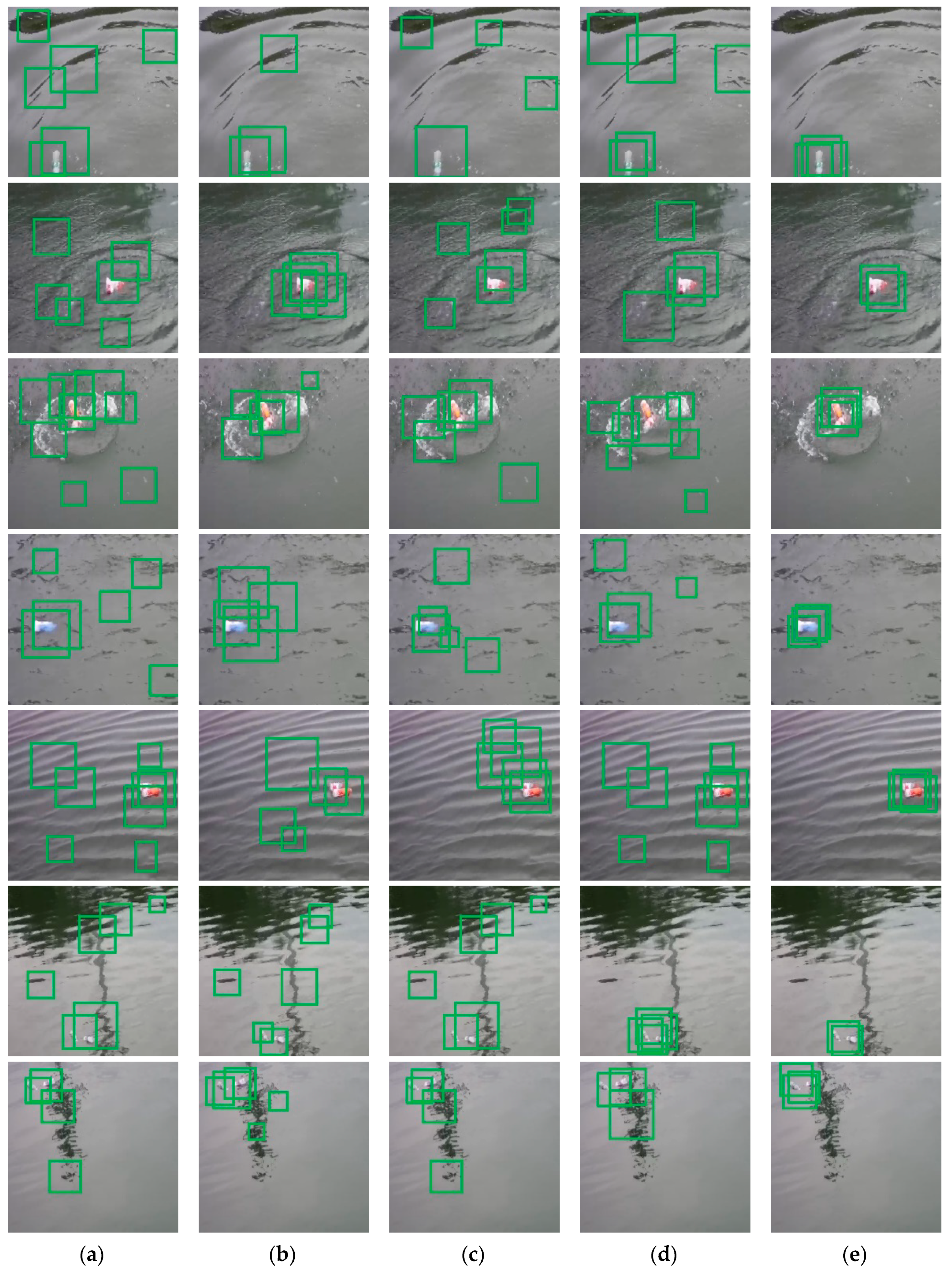
3.2. Intuitive Results of Saliency Detection
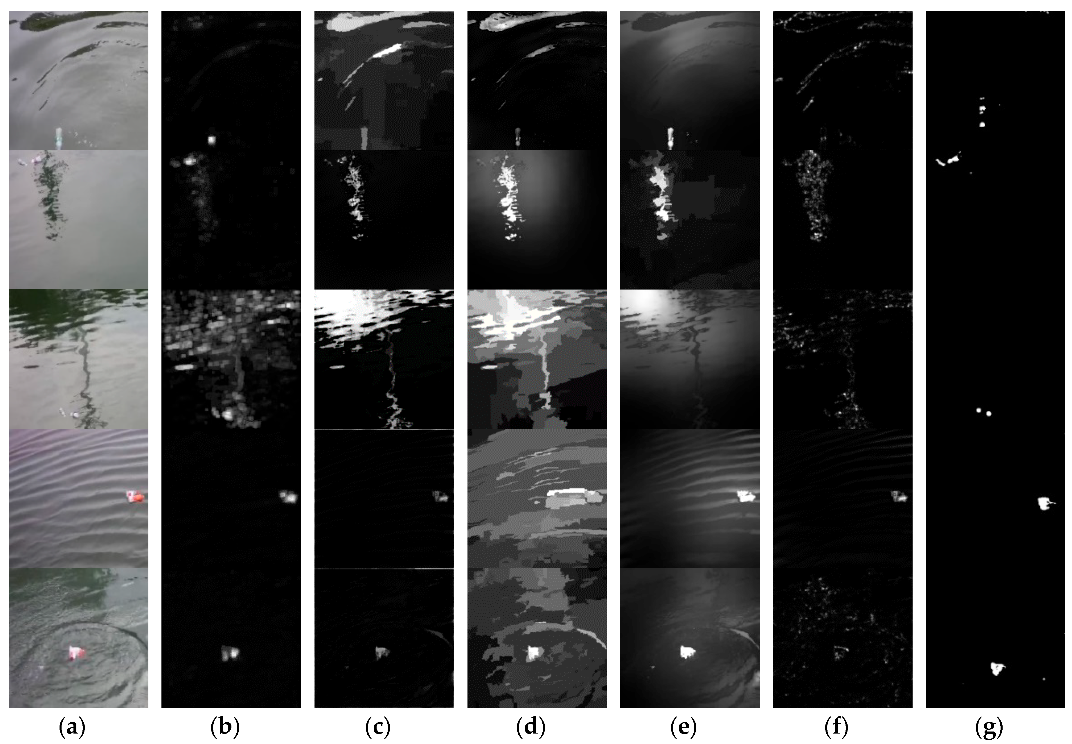
To demonstrate the effectiveness of our frequency-based saliency detection method, experiments with existing sample-free saliency detection methods are carried out. The results are shown in 5 challenging surface scenes, including huge reflections with big waves, striped ripples, slender reflections, huge circular waves under uneven illumination, and far-view reflections.
Figure 6 shows the results.
Figure 6b–f show the results of five popular sample-free saliency detection methods. In
Figure 6c,d, large ripples are mistaken for floating objects. In
Figure 6b,e, near-view reflections cause plenty of false detections. Though some ripples are removed by the frequency-based method SR, shown in
Figure 6f, important information of floating objects is removed as well. From these intuitive results, a preliminary conclusion can be drawn that the detection results of our method shown in
Figure 6g are optimal in the task of floating object detection with respect to various interference factors.
3.3. Intuitive Results of Combination
The results shown in the above subsections indicate that our spatial-based texture detection and frequency-based saliency detection can both obtain location information of floating objects. However, bounding boxes from texture detection are larger than the corresponding ground truths (due to small sample training), and the results of salient detection are smaller than the real sizes (due to the loss of contour information). Through combining bounding boxes from the two methods, closer results to the ground truths can be obtained. To demonstrate the effectiveness of the combination intuitively, results in five challenging scenes are shown in
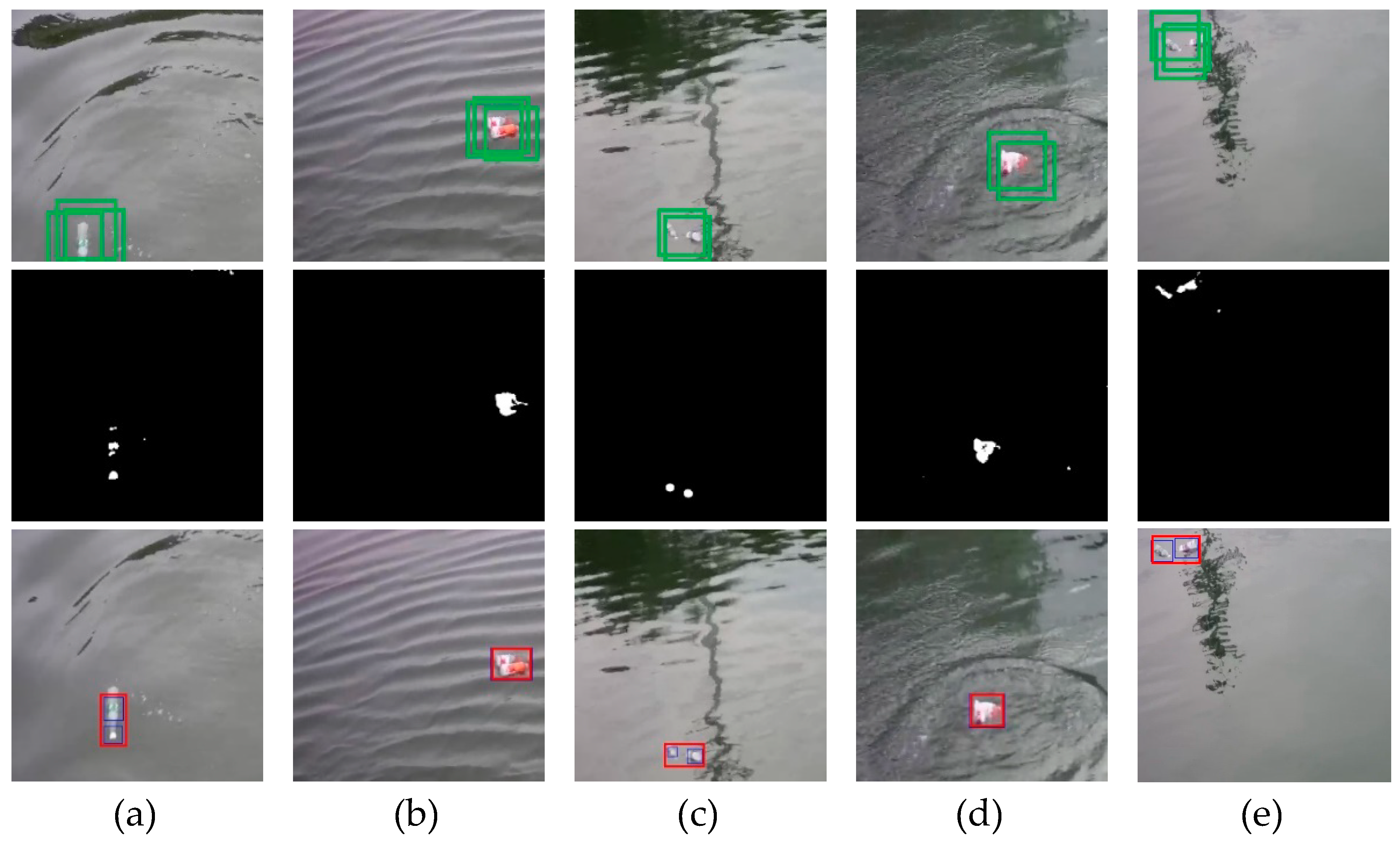
Figure 7.
In
Figure 7, the first line shows that our spatial-based texture detection is able to detect floating objects correctly, though their bounding boxes are larger than the ground truths. The second line shows that correct saliency maps with no redundancies are obtained by our frequency-based saliency detection, but some contours are removed (especially in
Figure 7a,c). The third line shows that the results of combination have the correct size and location information of floating objects, indicating that our combination strategy overcomes the shortcomings in different processing domains. Meanwhile, as shown in
Figure 7a–e, our method is robust in the five challenging scenes, and the final results are close to the ground truths.
3.4. Evaluation Metrics
To evaluate our results quantitatively, four popular evaluation metrics of object detection are calculated, i.e., Precision
P, Recall
R, F
1-Measure
F1, and average detection time
T. Precision and Recall are often a pair of contradiction measures. Generally speaking, when the Precision is high, the Recall tends to be low. Therefore, the comprehensive evaluation metric F
1-Measure is needed. Higher
F1 value indicates better performance of the detection model. The calculation methods of
P,
R, and
F1 are as follows:
where
TP and
TN denote the number of true positives and true negatives, respectively, while
FP and
FN denote the number of false positives and false negatives, respectively.
G is the number of ground truths, equal to the number of all positives. In our testing set consisting of 120 source images, the value of
G is 140 rather than 120, because some testing images contain multiple floating objects.
In our experiments, a result was considered a true positive only when the IoU calculated from the bounding box and its ground truth was higher than 0.8. This threshold guarantees the practicalities of the testing methods.
3.5. Parameters Selection
In the task of texture detection, FHOG feature can be extracted with different cell sizes, so it is necessary to find the optimal cell size through ablation experiments.
Table 1 shows the results of an ablation experiment to find the best cell size in feature extraction. As shown in
Table 1, texture detection with the cell size of 16 × 16 pixels has the highest precision and recall rate (88.24% and 96.4%, respectively), although they are close to the results when the cell size is 32 × 32 pixels. However, in terms of computational complexity, when the cell size is 16 × 16 pixels, the detection time is the shortest (0.333 seconds). This detection time is 0.108 seconds faster than the time when the cell size is 32 × 32 pixels. We concluded that bigger cells perform better in precision than the smaller ones until the size has reached 16 × 16, while the time consumption decreases as cell size increases except the size 32 × 32. Therefore, size 16 × 16 is the best choice.
In the task of saliency detection, ablation experiments are performed for the two tricky problems:
- (1)
what is the best weight of global saliency map in the fusion operation;
- (2)
how to solve the problem of high time consumption caused by matrix decomposition.
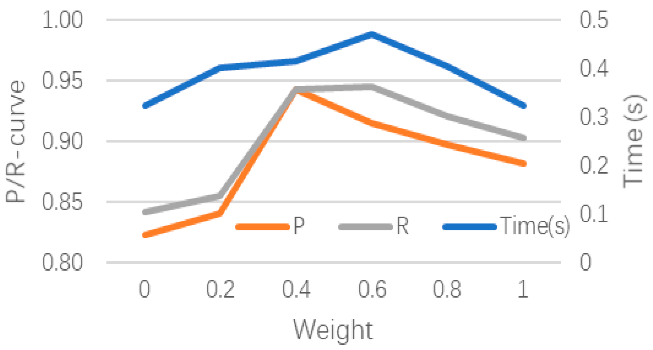
For the first problem, we made a comparison of the results of saliency detection for different global-map weights. As shown in
Figure 8, Precision peaks at the weight value of 0.4, and the Recall remains high at this value. Although the time consumption is very small when the weight is 1 or 0, its Precision and Recall are extremely low. Consequently, the optimal weight value of global saliency map is 0.4.
To solve the problem of time consuming in matrix decomposition, initial saliency maps are down-sampled before global decompositions, as smaller matrices make decompositions faster. Note that the initial saliency maps are not necessary to resize for local decompositions. We make a comparison of the results for different map sizes.
As shown in
Table 2, the smaller size for global decompositions not only makes the whole detection task have less time consumption, but also makes it have higher precision and recall rates. When the size is 48 × 48, all of the three parameters are optimal values, i.e., the highest precision rate (94.29%) and recall rate (94.29%), and the lowest time consumption (0.415 seconds). Note that the detection time of size 48 × 48 is 18.335 seconds faster than that of size 350 × 350, and the precision and recall rate are respectively 9.59% and 15.19% higher than those of size 350 × 350. The possible reason is that when an image is down-sampled, the calculated data is reduced, and some noises and redundant regions are removed as well.
3.6. Comparative Experiments
Comparative Experiments are carried out for the comprehensive evaluation. Among the existing methods in spatial domain, Wang [
5], Jang [
38], Tang [
7] are traditional image segmentation methods; HOG [
13], FHOG [
29], GLCM [
15], and LBP [
14] are texture detection methods; RC [
20], SF [
21], BMS [
22] are saliency detection methods; SSD300 [
17], the You Only Look Once method (YOLOv3) [
19], R-FCN [
16], RefineDet321 [
18] are popular object detection methods based on CNN. Due to the particularity of the research, only SR [
23], FT [
24], and MSS [
25] are the existing saliency detection methods in the frequency domain.
The experiments have the same configuration as below:
- (1)
Otsu Method [
8] for binarizations;
- (2)
cell size 16x16, block size 48x48 and classifier SVM for texture detections;
- (3)
backbone VGG16 and pre-training weight VGG16-VOC2007 [
35] for CNNs.
Table 3 shows the comparison of the results of existing methods.
In
Table 3, not only is the final result of our method (i.e., row 20) listed, but so is the result of spatial-based texture detection and the result of frequency-based saliency detection (i.e., row 8 and row 19, respectively). Unless otherwise specified, the result of our method refers to the final result. As shown in
Table 3, recalls of traditional image segmentation methods (i.e., rows 1–3) are lower than all the others because of interference factors. Texture detection methods (i.e., rows 4–8) have little time consumption, but their recalls are relatively low. It can be shown that our texture detection method (i.e., row 8) performs better than other texture-based methods, indicating that FHOG-GLCM is an effective hand-crafted texture feature. Frequency-based saliency detection methods (i.e., rows 16–19) are faster than the spatial-based ones (i.e., rows 13–15), and our saliency detection method (i.e., row 19) has the highest precision and recall rates among them. Although the popular CNN-based methods (i.e., rows 9–12) are close to ours in terms of Recall, our final method has higher precision with less time consumption.
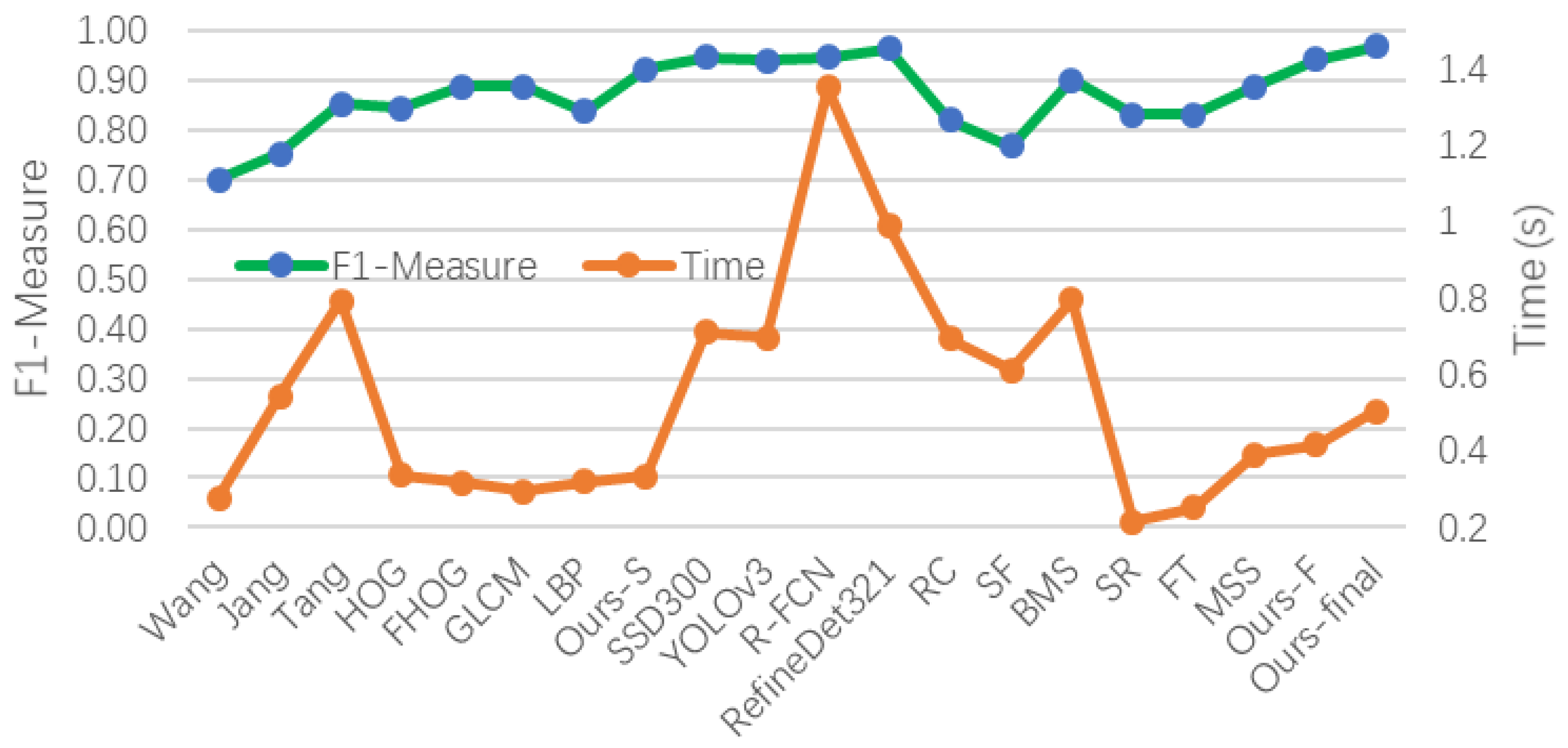
We calculated the size information of the objects detected by our final method. Statistical results show that in our testing set, when the accuracy is IoU >= 0.8, the largest object detected is 56 × 70 pixels and the smallest object is 27 × 31 pixels. To compensate for the inadequacy of the comparison of the above Precision and Recall (P-R) results, F1-Measures and time consumptions of all methods are intuitively shown in
Figure 9.
As shown in
Figure 9, the F
1-Measure of our final method (at around 0.95) is close to those of CNN-based methods, i.e., SSD300, YOLOv3, R-FCN, and RefineDet321. Meanwhile, the F
1-Measure of our final method is higher than those of traditional image segmentation methods, saliency detection methods, and other texture detection methods. In addition, time consumption of our method (at around 0.5 seconds) is much smaller than those of CNN-based methods. All the experimental results indicate that the overall performance of this method is the best one.
4. Conclusions
Aiming at the problem of floating object detection for the surface cleaning robot in the case of small sample acquisition and interferences factors from waves, reflections, and uneven illumination, an effective detection method is proposed. The method combines texture detection in spatial domain and saliency detection in frequency domain.
In texture detection, a useful combination of hand-crafted texture features is implemented. Compared with 4 traditional texture detection methods, precision of our texture detection is 88.24%, recall is 96.43% (IoU >= 0.8), F1-Measure is 0.92, and average detection time is 0.333 seconds, which demonstrates that our texture feature (FHOG-GLCM) describes floating objects effectively and efficiently.
In saliency detection, the proposed method combines frequency-domain processing and low-rank decomposition. Compared with six traditional saliency detection methods, the precision of our saliency detection is 94.29%, the recall is 94.29% (IoU >= 0.8), the F1-Measure is 0.89, and the average detection time is 0.415 seconds, which demonstrates that our saliency detection method performs better than other saliency detection methods in complex water scenes.
Compared with 17 existing methods including traditional image segmentation, saliency detection, hand-crafted feature classification, and CNN-based object detection, our final method has the highest precision (97.12%) and the highest recall (96.43%) with little time consumption (0.504 seconds). The results show the effectiveness of combining spatial and frequency domains, and the reliability and rapidity of our method of floating object detection for surface cleaning robots.


