Article

A MATLAB Package for Calculating Partial Derivatives of Surface-Wave Dispersion Curves by a Reduced Delta Matrix Method

Research Institute of Petroleum Exploration & Development, Lanzhou 730030, China
*
Author to whom correspondence should be addressed.
Appl. Sci. 2019, 9(23), 5214; https://doi.org/10.3390/app9235214
Submission received: 26 October 2019 / Revised: 26 November 2019 / Accepted: 27 November 2019 / Published: 30 November 2019
(This article belongs to the Special Issue Surface Waves for Monitoring of Materials at Different Scales)

Abstract

:
Various surface-wave exploration methods have become increasingly important tools in investigating the properties of subsurface structures. Inversion of the experimental dispersion curves is generally an indispensable component of these methods. Accurate and reliable calculation of partial derivatives of surface-wave dispersion curves with respect to parameters of subsurface layers is critical to the success of these approaches if the linearized inversion strategies are adopted. Here we present an open-source MATLAB package, named SWPD (Surface Wave Partial Derivative), for modeling surface-wave (both Rayleigh- and Love-wave) dispersion curves (both phase and group velocity) and particularly for computing their partial derivatives with high precision. The package is able to compute partial derivatives of phase velocity and of Love-wave group velocity analytically based on the combined use of the reduced delta matrix theory and the implicit function theorem. For partial derivatives of Rayleigh-wave group velocity, a hemi-analytical method is presented, which analytically calculates all the first-order partial differentiations and approximates the mixed second-order partial differentiation term with a central difference scheme. We provide examples to demonstrate the effectiveness of this package, and demo scripts are also provided for users to reproduce all results of this paper and thus to become familiar with the package as quickly as possible.

1. Introduction

Over the past three decades, a variety of surface-wave exploration methods has become an increasingly important means for inferring the properties of subsurface structures, especially in the near-surface region [1,2]. Compared with the commonly employed seismic body waves, the seismic surface waves (SWs), which primarily include Rayleigh and Love waves in land acquisition, usually propagate in the vicinity of the free surface and exhibit conspicuous dispersion characteristics in seismic records. This dispersion characteristic of SWs is generally delineated by the so-called phase- and/or group-velocity dispersion curves (DCs). The near-surface shear-wave velocities (Vs) can be obtained by inverting these DCs. The inverse problem of DCs, inherently nonlinear, can be solved by using global optimization methods, for instance, genetic algorithm [3], simulated annealing [4], particle swarm optimization [5], etc., or by using various linearized inversion strategies [1,6,7]. The success of either DCs inversion strategy is based on the accurate and efficient computation of surface-wave DCs. In addition, if the latter strategies are chosen, reliable calculations of partial derivatives (PDs) of DCs with respect to the parameters of subsurface strata are indispensable to create the Jacobian matrix (or the sensitivity matrix) in this class of strategies, especially due to the demand of their repeated calculations during the entire inversion process.
The efficient computation of surface-wave DCs benefits not only from the pioneering groundwork of Thomson and Haskell [8,9], but also from the rapid development of computer techniques after the 1960s. Inspired by Thomson and Haskell, numerous approaches have been proposed since then [10,11,12,13,14,15,16,17,18,19,20,21,22,23], particularly to remedy the issue of loss of numerical precision at high frequencies, which is an inherent shortcoming of Haskell’s theory (see reference [23] for more details). Among all these approaches, the one put forward by Dunkin [13] and its improved variants [14,23] are frequently utilized as the foundation of various surface-wave DCs inversion strategies due to their simplicity, efficiency, and effectiveness. Dunkin’s approach is based on the so-called delta matrix theory [13], with which the shortcoming of Haskell’s theory are thoroughly overcome.
Press et al. [10] developed the first computer program for computation of Rayleigh- and Love-wave DCs. In spite of the high efficiency in computing phase-velocity DCs, they applied the numerical differentiation of phase velocity to acquire the group velocity, which is a brute-force, low-precision, and unreliable method. The first category of analytical approaches for calculating the surface-wave group-velocity DCs and their PDs is based on the variational theory [24,25,26,27,28,29]. By virtue of Rayleigh’s principle, Jeffreys [24] first derived expressions for computing the group velocities of surface waves analytically; nonetheless, the PDs of DCs were approximated to the first order accuracy with numerical differentiation. Thereafter, the same idea was adapted to tackle more sophisticated cases, such as Takeuchi et al. [25,26], Anderson [27], Harkrider [28], and Aki et al. [29], just to name a few. On the other hand, to bypass the theoretical complexity of these approaches, Novotný introduced the implicit function method, another analytical approach, first for Love waves [30,31] and then for Rayleigh waves in the case of a layer overlying a half-space [32]. Then Urban et al. [33] succeeded in generalizing this approach to the case of multiple layers for Rayleigh waves. With the help of Knopoff’s algorithm [11,15,16], in combination with the implicit function method, they successfully acquired the analytical expressions for computing the PDs of Rayleigh-wave phase velocities, and the group velocities are also acquired by further using Rodi’s method [34].
To date, the most credit on this subject is given to researchers who focused on the scale of crustal seismology and who were mainly active before the 1990s. However, with the flourishment of the surface-wave methods for near surface characterization [1,2,3,4,5,6,7], this subject has regained new interest in recent years. For example, Cercato recently applied the reduced delta matrix method along with the implicit function theory to achieve the analytical computation of PDs of Rayleigh-wave ellipticity [35] as well as the necessary phase velocity [36]. In order to increase the computational efficiency, he formulated the PDs of Rayleigh-wave phase velocity in a vector-transferring manner instead of the matrix multiplication. Nevertheless, this computational manner makes it intractable to further calculate the PDs of group velocity analytically since more complex second-order partial differentiations must be dealt with. In addition, he only considered the Rayleigh waves in the study. Due to the complexity of this analytical method, it is not widely used in current surface-wave linearized inversion strategies and many researchers have resorted to the global optimization methods as previously mentioned, bypassing the calculation of PDs. However, these methods require a large amount of calculation, particularly when thousands of DCs need to be inverted, as in the context of oil seismic exploration.
Based on the above-mentioned reasons, here we rederive a set of new analytical expressions in the manner of matrix multiplication and present the relevant algorithms to compute the PDs of surface-wave DCs. This work can be taken as another option or a complement to the previous studies. We derive the relevant formulas and algorithms in such another way that is more convenient and more straightforward for considering all of the cases (Love and Rayleigh waves; phase and group velocity). Furthermore, we develop an open-source MATLAB package called SWPD (Surface Waves Partial Derivatives) accompanying this paper, and it has the following merits: (i) it is able to deal with both Rayleigh and Love waves; (ii) it can calculate the PDs of surface-wave phase-velocity DCs analytically or accomplish the calculations for Rayleigh-wave group-velocity DCs by a hemi-analytical method with high precision; (iii) all the relevant expressions and algorithms are derived from a widely accepted frame (i.e., the reduced delta matrix method), which makes the package easy to use and to be extended. It is worth mentioning that the hemi-analytical method is a compromise: it calculates all the relevant first-order PDs analytically and approximates the only second-order mixed PD term with a central finite-difference scheme. By doing so, we still can obtain satisfying results comparable to the analytical approach [32], meanwhile avoiding the intricate analytical derivations for the second-order term.
We first outline the reduced delta matrix theory and its application in modeling the surface-wave phase-velocity DCs. We then present the algorithms and related formulas to calculate analytically the PDs of the phase velocity (Section 3). Next, both the fully analytical and the hemi-analytical approaches for calculating the PDs of the surface-wave group velocity are elaborated (Section 4). After that, we also describe the accompanying MATLAB code with focus on some key scripts or functions (Section 5). Last, four models are utilized for verification of our method and of the package (Section 6).

2. Computations of Surface-Wave Phase-Velocity DCs Based on the Reduced Delta Matrix Method

We first give a brief overview of the reduced delta matrix method [14,23,35] since it constitutes the foundation of the following sections. We strictly follow the formulism of Buchen et al. [23] due to his modern mathematical representations compared with other earlier studies.
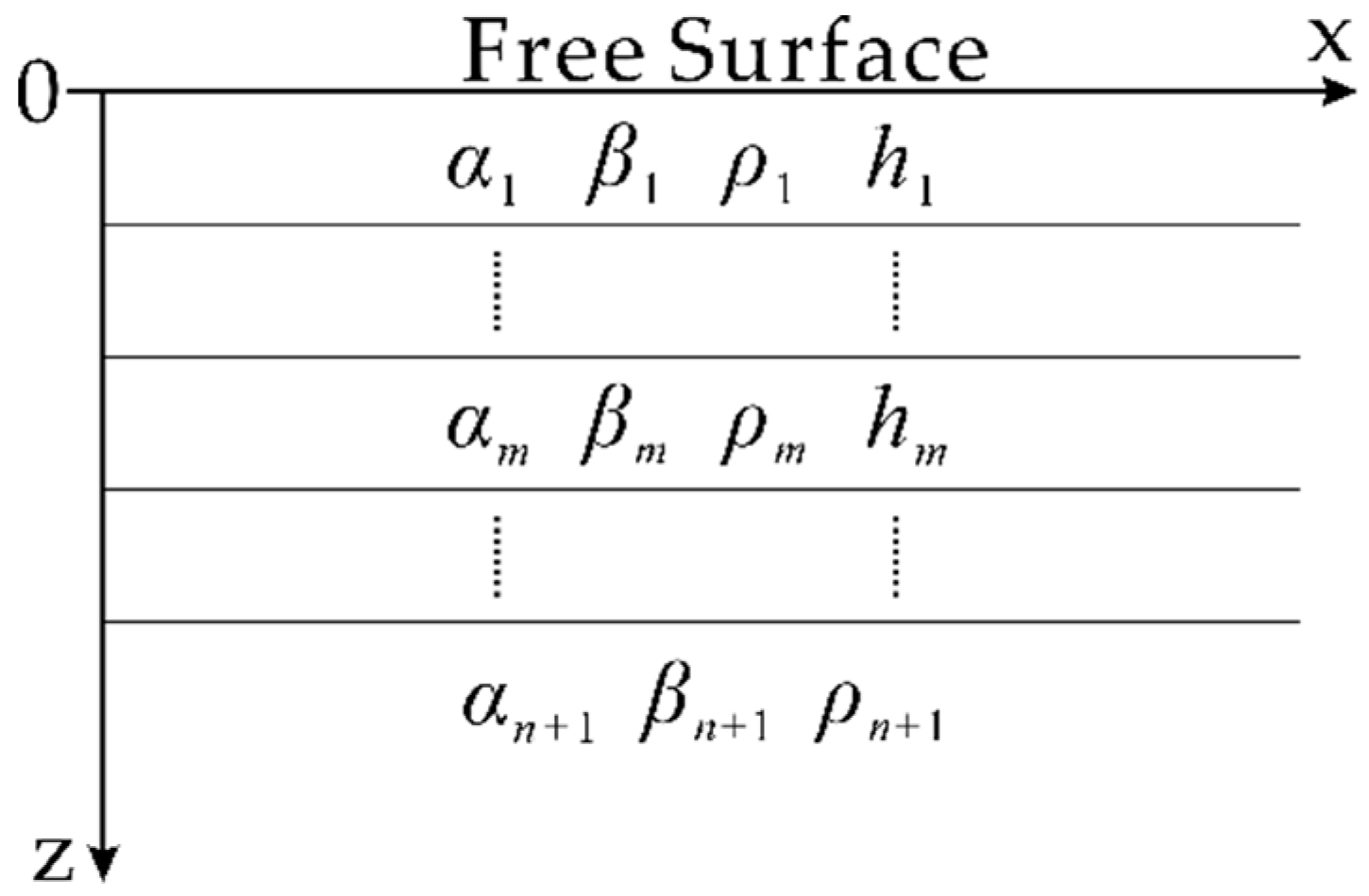
This research involved a multilayered earth model (Figure 1), which consists of many homogeneous, isotropic, and elastic layers that overlie a half-space and lie beneath a free surface. Each layer is denoted by the P-wave velocity α m , the S-wave velocity β m , the density ρ m and the thickness h m . According to the reduced delta matrix method, the surface-wave secular (or dispersion) equation F can be described as an implicit function by the delta matrix recursion:
X ¯ m + 1 * = X ¯ m * T ¯ m * ,   m = 1 , 2 , , n F ( ω , c ) = X ¯ n + 1 * V ¯ n + 1 * = 0
where ω is the angular frequency, c is the phase velocity, m is the sequence number for layers, and n + 1 indicates the half-space. X ¯ m * is a row vector with different lengths depending on which wave (Love or Rayleigh wave) is concerned. T ¯ m * and V ¯ n + 1 * can be regarded as the reduced delta matrices corresponding to the layer m and the half-space, respectively. The elements of these three matrices are listed in Appendix A. In order to obtain the phase-velocity DCs, the frequencies or periods of interest are substituted into (1), followed by a root-finding procedure consisting of the integrated use of the bisection method and the Brent method in this paper. Generally, there are multiple solutions or roots at a certain frequency or period, and the root corresponding to the lowest c is the fundamental mode while other roots are the higher modes.

3. Computation of PDs of Surface-Wave Phase Velocities

In this section, we derive the algorithms, based on matrix multiplication, for computation of PDs of surface-wave phase velocities. In fact, the surface-wave dispersion equation F also depends on the physical parameters of the subsurface. To facilitate the description, let a vector Q indicate these parameters [35]. In other words,
Q R = ( α 1 , , α n + 1 , β 1 , , β n + 1 , ρ 1 , , ρ n + 1 , h 1 , , h n )
for the case of Rayleigh waves, or
Q L = ( β 1 , , β n + 1 , ρ 1 , , ρ n + 1 , h 1 , , h n )
for the case of Love waves. Hence, the completed form of F is
F ( ω , c , Q R ) = 0   or   F ( ω , c , Q L ) = 0 .
Suppose we want to compute c / p t , where p represents a generic physical parameter such as α, β, ρ, or h of the objective layer t. Making use of the implicit function theory, c / p t can be written as:
c / p t = F / p t F / c .
In the following, let us first consider F / c . On the basis of recursion (1) and the derivative rules, the expression for F / c can be derived as follows:
F / c = X ¯ n + 1 * c V ¯ n + 1 * + X ¯ n + 1 * V ¯ n + 1 * c .
Obviously, the calculation of V ¯ n + 1 * / c is straightforward, whereas X ¯ n + 1 * / c has to be calculated recursively starting from the first layer via formula (1):
X ¯ m + 1 * / c = X ¯ m * c T ¯ m * + X ¯ m * T ¯ m * c ,   m = 1 , 2 , , n .
For a clearer description of the algorithm (Table 1), let us introduce a new vector, i.e., Y ¯ m * = X ¯ m * / c , thus (6) can be reformulated as follows:
Y ¯ m + 1 * = Y ¯ m * T ¯ m * + X ¯ m * T ¯ m * c ,   m = 1 , 2 , , n .
This is obviously a zero vector as X ¯ 1 * is a constant vector. A similar algorithm can be derived for F / p t (Table 2), except that there are two cases that need to be taken into account according to the sequence number t (whether it equals to n + 1). Therefore, by using these two algorithms and (4) in conjunction, the PDs can be computed analytically. We only show the elements of V ¯ n + 1 * / c , T ¯ m * / c , V ¯ n + 1 * / p n + 1 , and T ¯ t * / p t for Love waves in Appendix B. As for Rayleigh waves, due to the lengthy formulas and the limited space, we suggest readers go directly to the source code according to the description in Section 5.

4. Computation of PDs of Surface-Wave Group Velocities

The group velocity is the propagation velocity of the energy of a wave packet and is related to the phase velocity by the following expression [31]:
U = ω / k = c / [ 1 ( ω / c ) c / ω ]
where k is the angular wavenumber. Therefore, if certain modes of phase-velocity DCs have been acquired, then the corresponding group-velocity DCs can be calculated by (8).
Two different approaches are implemented in the package: (i) a fully analytical method via implicit function theory (for Love waves); (ii) a hemi-analytical method (for Rayleigh waves). In the following, we will explain both approaches, respectively.

4.1. Fully Analytical Method

The first order derivative c / ω in (8) also can be calculated by using the implicit function theory:
c / ω = F / ω F / c .
Although the pseudo-code in Table 1 is for F / c , it is apparently applicable to F / ω , provided that c is replaced by ω. Similarly, the PDs of group velocity with respect to certain generic physical parameter p of the objective layer t can be derived from (8) [30,31,32,33,36]:
U p t = U c ( 2 U c ) c p t + ω U 2 c 2 2 c ω p t .
The second-order mixed partial derivative in (10) can be derived by further differentiating (4) with respect to ω [31]:
2 c ω p t = [ 2 F ω p t + 2 F ω c c p t + ( 2 F c p t + 2 F c 2 c p t ) c ω ] / F c .
In the following, we take 2 F c 2 as an example to illustrate how to calculate the second-order partial derivatives analytically. As for 2 F c p t , 2 F ω p t , and 2 F ω c , they can be calculated in the same way.
The computational procedure for F / c (Table 1) can be performed in a recursive manner:
X ¯ m + 1 * = X ¯ m * T ¯ m * ,   m = 1 , 2 , , n ; Y ¯ m + 1 * = Y ¯ m * T ¯ m * + X ¯ m * T ¯ m * c ,   m = 1 , 2 , , n ; F / c = Y ¯ n + 1 * V ¯ n + 1 * + X ¯ n + 1 * V ¯ n + 1 * c .
Therefore, we differentiate the last expression above with respect to c and thus obtain
2 F / c 2 = Y ¯ n + 1 * c V ¯ n + 1 * + 2 Y ¯ n + 1 * V ¯ n + 1 * c + X ¯ n + 1 * 2 V ¯ n + 1 * c 2 .
Then, in order to obtain Y ¯ n + 1 * / c , we shall resort to the second expression in (12):
Y ¯ m + 1 * / c = Y ¯ m * c T ¯ m * + 2 Y ¯ m * T ¯ m * c + X ¯ m * 2 T ¯ m * c 2 , m = 1 , 2 , , n .
Similarly, if we introduce a new vector Z ¯ m * = Y ¯ m * / c , then (14) can be reformulated as follows:
Z ¯ m + 1 * = Z ¯ m * T ¯ m * + 2 Y ¯ m * T ¯ m * c + X ¯ m * 2 T ¯ m * c 2 , m = 1 , 2 , , n .
Obviously, Z ¯ 1 * is a zero vector as well. Thus, by taking advantage of (12), (15), and (13), we can finally implement the analytical computation of 2 F / c 2 (Table 3). See Appendix C for the elements of 2 T ¯ m * / c 2 and of 2 V ¯ n + 1 * / c 2 for Love waves.

4.2. Hemi-Analytical Method

In the fully analytical method, the crucial second-order partial derivative term 2 c ω p t in (10) is substituted by (11) and then solved via some recursive procedures. In contrast, the hemi-analytical method approximates this term with a central finite-difference scheme [36], a procedure which will be briefly reviewed in the following.
Suppose that the partial derivative U / p t is desired at the angular frequency ω 0 and that the phase velocity c 0 and group velocity U 0 are computed at ω 0 . Define two other frequencies around ω 0 : ω + 1 = ω 0 e + δ and ω 1 = ω 0 e δ . δ is a small quantity, denoting a perturbation of log ω ; see [36] for a more detailed explanation. And suppose the quantities c + 1 , U + 1 , and c + 1 / p t are corresponding to ω + 1 and have been obtained. The same hypothesis is applied to the quantities c 1 , U 1 , and c 1 / p t at ω 1 . Then the PD of the group velocity at ω 0 can be computed via
U 0 / p t = U 0 c 0 ( 2 U 0 c 0 ) c 0 p t + U 0 2 c 0 2 ( c + 1 / p t c 1 / p t 2 δ )
We call (16) ‘hemi-analytical’ due to the fact that all the first-order partial derivatives and U 0 in (16) are computed by the analytical approach discussed previously, leaving only 2 c ω p t approximated by the central finite-difference.

5. Package Description

SWPD, written in MATLAB, consists of two independent parts for dealing with Rayleigh and Love wave respectively. Most source files of the package are written for implementing the partial differentiations of matrix T ¯ m * and of dispersion function F. To make it clearer, we list these files in Table A1 and Table A2, respectively. As shown in these two Tables, for example, reduced_delta_love.m and reduced_delta.m implement the delta matrix recursion (1) for Love and Rayleigh waves, respectively. Files reduced_delta_love_dfdc.m and reduced_delta_dfdc.m perform the pseudo-code in Table 1 to yield the PDs of the dispersion function F with respect to c. When F / β is desired (as the pseudo-code shown in Table 2), one can go to files reduced_delta_love_dfdb.m and reduced_delta_dfdb.m. Similarly, reduced_delta_love_dfdcc.m has implemented the algorithm in Table 3. In summary, all the main *.m files that perform partial differentiations are summarized in Table A2 and they need to call the sub-function files in Table A1 to accomplish the relevant computations.
Besides those scripts described above, there are a few other *.m files deserving to be mentioned. rayleighphase.m and lovephase.m are used to model the multimodal phase-velocity DCs. The hemi-analytical method has been implemented in four *.m files whose filenames contain the string ‘rodi’. In fact, we have included five demo scripts, whose filenames begin with the string ‘demo’. Hence, one can replicate all figures of this paper by running the demo scripts directly and so to become familiar with SWPD as quickly as possible.

6. Examples

6.1. Love-Wave Case

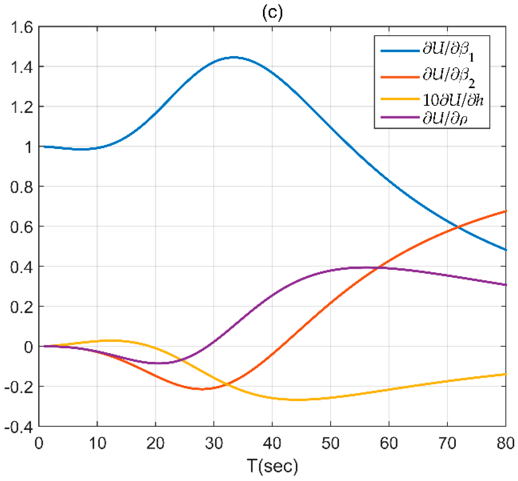
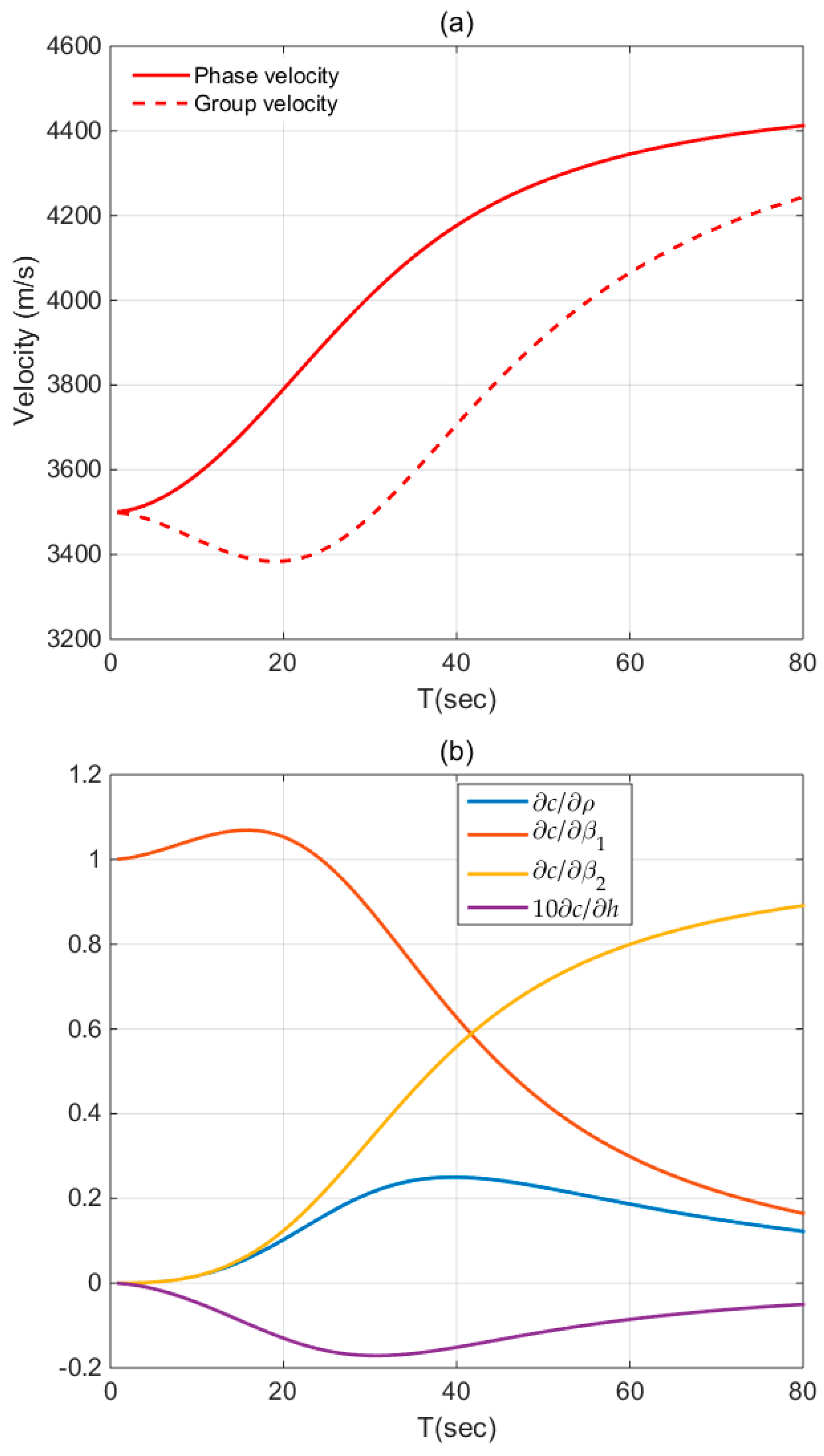
First, a two-layer model (Model Nov71 in Table 4) is chosen to demonstrate the validity of the proposed algorithms and of the developed code for the case of Love waves. Figure 2 shows the computational results for Model Nov71. Although the package is capable of modeling multiple modes, we only show the results of the fundamental mode for comparison with the published studies [30,31]. It is noteworthy that, in Figure 2 we plot curves of 10 × c / h and 10 × U / h instead of their original values due to their large differences in quantitative values compared to the other derivatives, so to make the changes of these two curves recognizable. In addition, in the work of Novotný [31], to facilitate the derivation of the analytical formulism specifically for the case of two layers, he introduced a dimensionless quantity ρ = ρ 2 / ρ 1 and plotted the curves of c / ρ and U / ρ . Therefore, to obtain the same curves, we have made use of the chain rule:
c / ρ = c ρ 2 ρ 2 ρ = ρ 1 c ρ 2   and   U / ρ = U ρ 2 ρ 2 ρ = ρ 1 U ρ 2 .
Obviously, the computational results in Figure 2 are rather consistent with the work of Novotný [31] (see Figure 1, Figure 2 and Figure 3 of his paper). To verify the correctness of these results more clearly, the relevant quantities calculated at 20, 30, and 40 s are shown in Table 5 (related to phase velocity) and in Table 6 (related to group velocity), respectively. As shown in the Tables, they are in good agreement with the outcomes from Novotný [31] (see Table 1 and Table 2 of his paper).
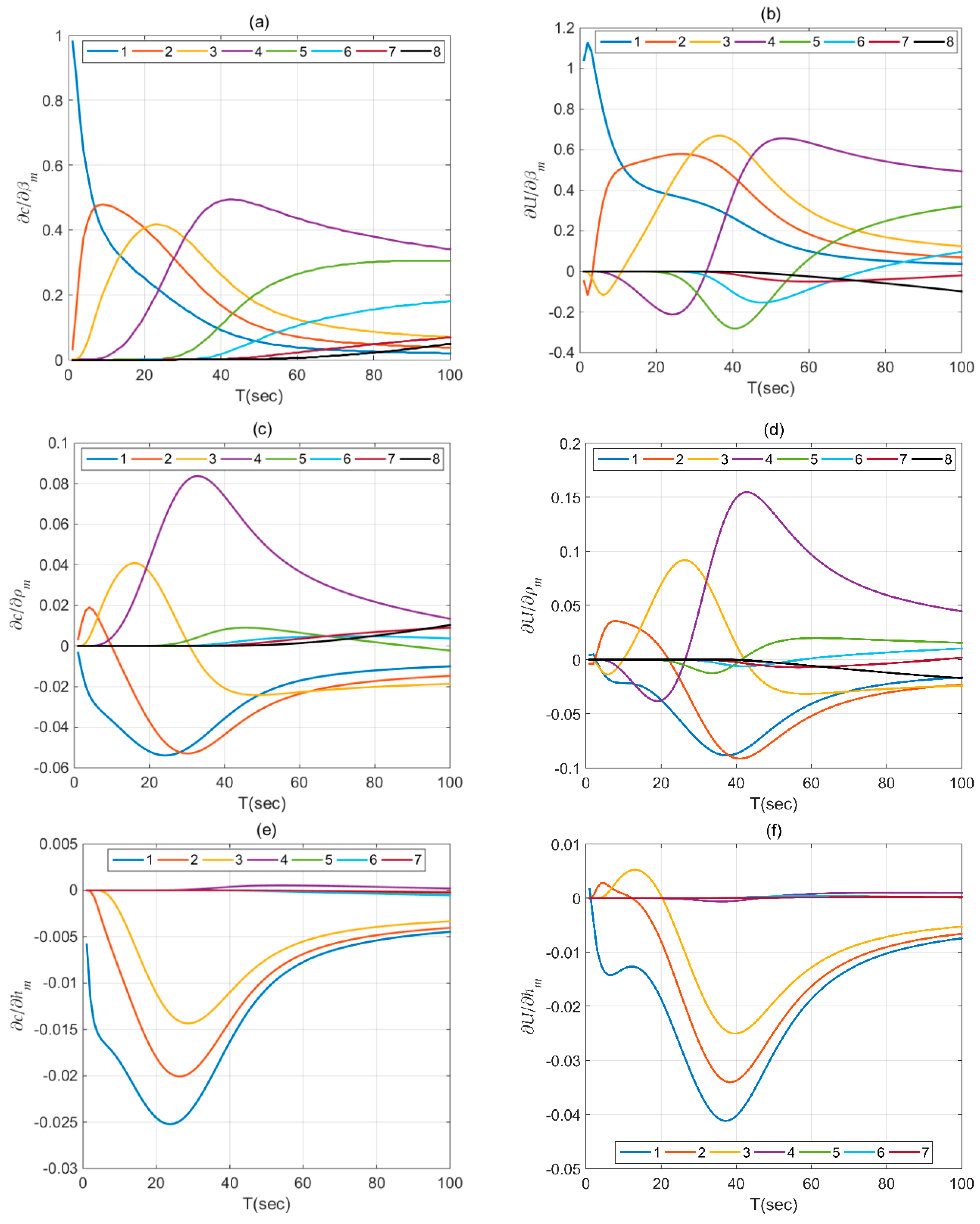
Next, an eight-layer model (Model Nov70 in Table 4) is used for a further verification. The PDs of the fundamental-mode phase and group velocity are presented in Figure 3. Also, the results calculated at 20 and 40 s for individual layer are listed in Table 7 and Table 8 for detailed comparisons. It should be pointed out that Novotný [30] (Figure 1, Figure 2, Figure 3, Figure 4 and Figure 5 in that paper) did not plot some partial derivatives because of their too small absolute values, whereas we plot all partial derivatives, regardless of their magnitude. After comparison, we can conclude that the results for the case of multiple layers are also satisfactory.

6.2. Rayleigh-Wave Case

6.2.1. A Two-Layer Model

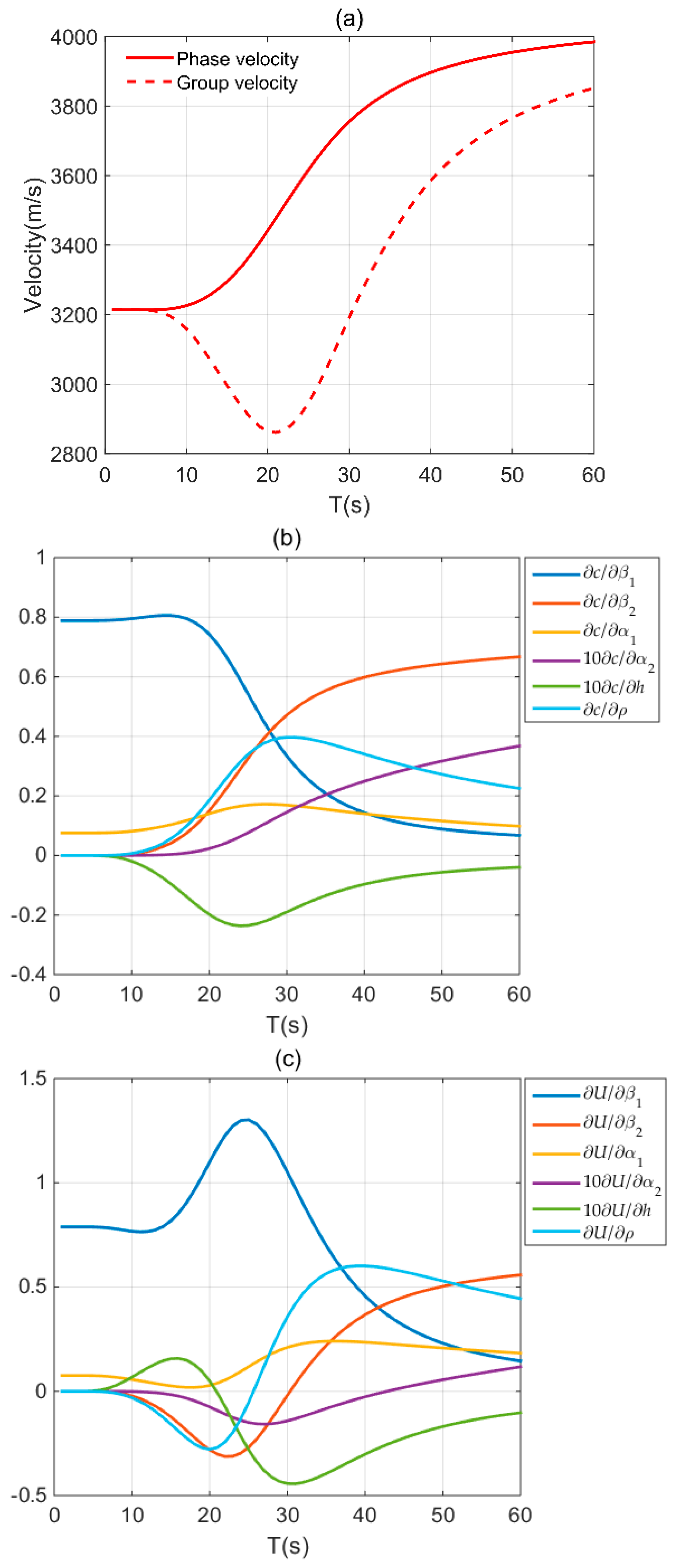
Let us further consider Rayleigh waves. In the first example, we adopt a two-layer model that is almost the same with Model Nov71, except that the P-wave velocities of the layers are also taken into account ( α 1 = 6000 m∙s−1 and α 2 = 8000 m∙s−1) [32]. Figure 4 displays the related computational outcomes of fundamental-mode phase and group velocity. They show apparently good agreements with [32] (Figure 1, Figure 2 and Figure 3 in that paper). Table 9 also shows the relevant results of phase velocity at three different periods for a detailed comparison. It is worth to point out that although we have used difference approximation while coping with the PDs of group velocity, the quantities acquired by the hemi-analytical approach still can be accurate to five decimal places as compared to the fully analytical approach [32] (see Figure 4c and Table 10). Hence, the hemi-analytical approach is a rather effective and accurate scheme that can be used to construct the Jacobian matrix while the linearized inversion of Rayleigh-wave group-velocity DCs is to be conducted.

6.2.2. A Six-Layer Model

All of the above-mentioned models are aimed at the scale of crustal seismology. In this example, we chose a near-surface six-layer model (Table 11) to demonstrate the applicability and effectiveness of our code at the scale of near-surface geophysics. This model was also chosen because some researchers have reported their results [1,35].
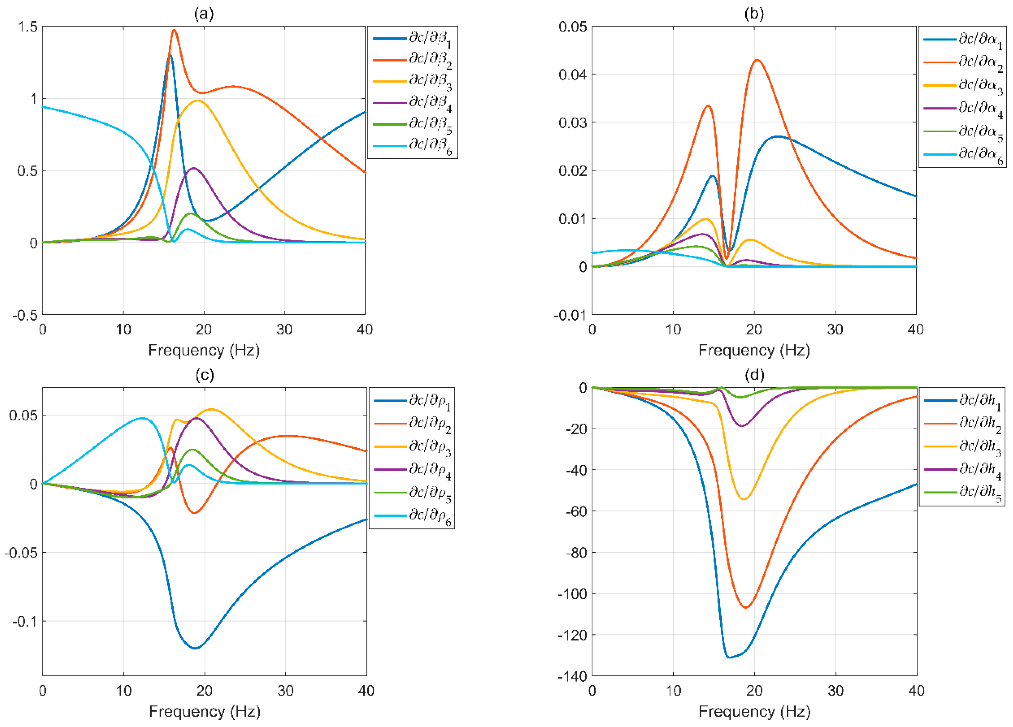
As shown in Figure 5, the analytical PDs of the fundamental-mode Rayleigh-wave phase velocity of the six-layer model are quite consistent with [35] (Figure 3, Figure 4 and Figure 5 of his paper). In order to show more details, as an example, the PDs with respect to the S-wave velocities at five different frequencies, along with the outcomes from other researchers, are presented in Table 12 (modified from [35]). Individual column of these matrices corresponds to a layer, whereas individual row corresponds to a frequency. Obviously, only the numerical results from Lai and Rix [6] show a certain lack of accuracy due to the adopted numerical integration in their code [35], whereas other results (including our result) are quite similar.

7. Discussion and Conclusions

The accurate and reliable calculation of PDs of surface-wave DCs is an essential component of any linearized inversion strategy based on surface-wave DCs. In this paper, we have rederived a series of algorithms and the related expressions based on the reduced delta matrix theory to compute analytically the PDs of surface-wave (both Love and Rayleigh waves) phase-velocity DCs. Moreover, we have also applied this analytical method to compute the PDs of Love-wave group velocity. Although Equations (9)–(15) constitute an abstract framework applicable to both waves, the derivation of all the second-order mixed PDs for Rayleigh waves could be rather difficult. Therefore, we have implemented a high-precision hemi-analytical method, which computes all the first-order partial differentiation analytically (Section 3) and approximates the only mixed second-order partial differentiation term with a central finite-difference scheme. For the fully analytical computation of Rayleigh-wave group-velocity PDs, Novotný et al. [32] is the only work we could find, despite the fact that only the case of two-layer model was studied due to the complexity of this problem. The comparison (Section 6.2.1) demonstrates that this mixed computational strategy is satisfying, with a comparable accuracy to five decimal places, as shown in Table 10.
An open-source MATLAB package named SWPD has been developed accompanying this paper. All examples in this paper have been validated by comparing with the results of previous studies, and all the results computed by our package are satisfactory with rather high precision. Therefore, it has been demonstrated that the analytical expressions and the algorithms derived in this paper are effective. Also, these examples can be reproduced by other users with the help of four demo scripts in the package. Upon becoming familiar with this package, people could modify and extend it without any difficulty, including any further development of the surface-wave linearized inversion strategy. We think this package could be a useful tool for people who are engaged in the field of near-surface geophysics, especially for those who are interested in surface-wave exploration methods.
Author Contributions

Conceptualization, D.W., X.W. and Q.S.; Methodology, D.W., X.W. and Q.S.; Software, D.W.; Formal analysis, D.W., X.W., Q.S. and T.Z.; Funding acquisition, X.W. and Q.S.; Investigation, D.W., Q.S. and T.Z.; Project administration, X.W., Q.S. and T.Z.; Resources, X.W. and Q.S.; Validation, D.W., X.W., Q.S. and T.Z.; Writing—original draft, D.W.; Writing—review & editing D.W., X.W., Q.S. and T.Z.

Funding

This research is funded by the National Science and Technology Major Project of the Ministry of Science and Technology of China “the study of key geophysical exploration technologies for Lower Palaeozoic Erathem-Precambrian basement tectonics (2016ZX05004-003)”

Acknowledgments

We are grateful to the valuable comments by the anonymous reviewers, which have helped improve this manuscript.

Conflicts of Interest

The authors declare no conflict of interest.

Appendix A

The expressions presented below are adapted from Buchen & Ben-Hador [23] just for convenience of reference.
Basic physical quantities employed:
  • ω = angular frequency
  • c = phase velocity
  • k = ω / c = angular wavenumber
  • i = 1 = imaginary unit
Basic derived quantities employed for the m-th layer (subscript m is omitted for simplicity):
r = { 1 c 2 / α 2 , c < α i c 2 / α 2 1 , c > α
C α = { cosh ( k r h ) , c < α cos ( i k r h ) , c > α
C β = { cosh ( k s h ) , c < β cos ( i k s h ) , c > β
S α = { sinh ( k r h ) , c < α i sin ( i k r h ) , c > α
S β = { sinh ( k s h ) , c < β i sin ( i k s h ) , c > β
γ = β 2 / c 2 ,   t = 2 1 / γ ,   μ = ρ β 2
F o r   L o v e   w a v e s : F o r   R a y l e i g h   w a v e s : X ¯ 1 * = [ 0 1 ] X ¯ 1 * = [ 0 0 0 0 1 ] T ¯ m * = [ C β S β μ s μ s S β C β ] m T ¯ m * = [ T ¯ 11 T ¯ 12 T ¯ 13 T ¯ 14 T ¯ 16 2 T ¯ 21 2 T ¯ 22 1 2 T ¯ 23 2 T ¯ 24 2 T ¯ 26 T ¯ 31 T ¯ 32 T ¯ 33 T ¯ 34 T ¯ 36 T ¯ 41 T ¯ 42 T ¯ 43 T ¯ 44 T ¯ 46 T ¯ 61 T ¯ 62 T ¯ 63 T ¯ 64 T ¯ 66 ] m V ¯ n + 1 * = [ 1 μ s ] n + 1 T V ¯ n + 1 * = [ 1 r s 2 μ ( t 2 r s ) μ s ( 2 t ) μ r ( 2 t ) μ 2 ( 4 r s t 2 ) ] n + 1 T
where the superscript T means the matrix transpose.
The elements of matrix T ¯ m * for Rayleigh wave:
Q j = ( t j r s + 2 j r s ) S α S β ,   0 j 4
T ¯ 11 = γ 2 [ 4 t + ( t 2 + 4 ) C α C β Q 2 ]
T ¯ 12 = γ 2 μ [ ( 2 + t ) ( 1 C α C β ) + Q 1 ]
T ¯ 13 = γ μ ( C α S β / s r S α C β )
T ¯ 14 = γ μ ( s C α S β S α C β / r )
T ¯ 16 = γ 2 μ 2 [ 2 ( 1 C α C β ) + Q 0 ]
T ¯ 21 = μ γ 2 [ 2 t ( t + 2 ) ( 1 C α C β ) Q 3 ]
T ¯ 22 = 1 + C α C β T ¯ 11
T ¯ 23 = γ ( t C α S β / s 2 r S α C β )
T ¯ 24 = γ ( 2 s C α S β t S α C β / r )
T ¯ 26 = T ¯ 12
T ¯ 31 = μ γ ( 4 s C α S β t 2 S α C β / r )
T ¯ 32 = T ¯ 24
T ¯ 33 = C α C β
T ¯ 34 = s S α S β / r
T ¯ 36 = T ¯ 14
T ¯ 41 = μ γ ( t 2 C α S β / s 4 r S α C β )
T ¯ 42 = T ¯ 23
T ¯ 43 = r S α S β / s
T ¯ 44 = T ¯ 33
T ¯ 46 = T ¯ 13
T ¯ 61 = μ 2 γ 2 [ 8 t 2 ( 1 C α C β ) + Q 4 ]
T ¯ 62 = T ¯ 21
T ¯ 63 = T ¯ 41
T ¯ 64 = T ¯ 31
T ¯ 66 = T ¯ 11

Appendix B

The expressions listed below are used for the construction of the first-order PDs of matrices T ¯ m * and V ¯ n + 1 * for Love waves. For clarity, we use the same notation as Cercato [35], i.e., the prime mark (e.g., s ) is used exclusively to indicate PD with respect to phase velocity c, whereas any subscript indicates PD with respect to that parameter (e.g., s β = s / β and ( C β ) β = C β / β ).
Define an intermediate variable
s 0 = 1 c 2 / β 2
For T ¯ m * / c :
s 0 = 2 c / β 2
s = 0.5 s 0 / s
C β = S β k h ( s s / c )
s β = C β k h ( s s / c )
T ¯ m * / c = [ C β S β s S β s μ s 2 μ ( s S β + s s β ) C β ]
For V ¯ n + 1 * / c :
V ¯ n + 1 * / c = [ 0 s μ ] T
For T ¯ m * / β :
( s 0 ) β = 2 c 2 / β 3
μ β = 2 ρ β
s β = 0.5 ( s 0 ) β / s
( C β ) β = k h S β s β ,     ( S β ) β = k h C β s β
T ¯ m * / β = [ ( C β ) β μ β S β μ 2 s + ( S β ) β s S β s β μ s 2 μ β s S β + μ ( S β s β + s ( S β ) β ) ( C β ) β ]
For V ¯ n + 1 * / β :
V ¯ n + 1 * / β = [ 0 μ β s + μ s β ] T
For T ¯ m * / ρ :
μ ρ = β 2
T ¯ m * / ρ = [ 0 μ ρ S β μ 2 s μ ρ s S β 0 ]
For V ¯ n + 1 * / ρ :
V ¯ n + 1 * / ρ = [ 0 μ ρ s ] T
For T ¯ m * / h :
( C β ) h = S β k s ,     ( S β ) h = C β k s
T ¯ m * / h = [ ( C β ) h ( S β ) h μ s μ s ( S β ) h ( C β ) h ]

Appendix C

The double-prime mark is used for indicating the second-order PDs with respect to c for Love waves.
s 0 = 2 / β 2
s = ( 0.5 s 0 ( s ) 2 ) / s
C β = k h { ( S β S β c ) ( s s c ) + S β [ s ( s s c ) 1 c ] }
S β = k h { ( C β C β c ) ( s s c ) + C β [ s ( s s c ) 1 c ] }
For 2 T ¯ m * / c 2 :
y = S β s S β s
y = S β s S β s
2 T ¯ m * / c 2 = [ C β y s 2 2 y s s μ s 4 μ ( s S β + 2 s S β + s S β ) C β ]
For 2 V ¯ n + 1 * / c 2 :
2 V ¯ n + 1 * / c 2 = [ 0 s μ ] T

Appendix D

Table A1. MATLAB *.m files that compute matrix T ¯ m * and its partial derivatives (PDs).
RoleLove wavesRayleigh waves
T ¯ m * get_T_love.mget_T.m
T ¯ m * / α get_dTda.m
T ¯ m * / β get_dTdb_love.mget_dTdb.m
2 T ¯ m * β c get_dTdbc_love.m
2 T ¯ m * β ω get_dTdbw_love.m
T ¯ m * / c get_dTdc_love.mget_dTdc.m
2 T ¯ m * / c 2 get_dTdcc_love.m
T ¯ m * / ω get_dTdw_love.mget_dTdw.m
2 T ¯ m * ω c get_dTdwc_love.m
T ¯ m * / h get_dTdh_love.mget_dTdh.m
2 T ¯ m * h c get_dTdhc_love.m
2 T ¯ m * h ω get_dTdhw_love.m
T ¯ m * / ρ get_dTdrho_love.mget_dTdrho.m
2 T ¯ m * ρ c get_dTdrhoc_love.m
2 T ¯ m * ρ ω get_dTdrhow_love.m
Table A2. MATLAB *.m files that compute dispersion function F and its PDs.
RoleLove wavesRayleigh waves
F reduced_delta_love.mreduced_delta.m
F / α reduced_delta_dfda.m
F / β reduced_delta_love_dfdb.mreduced_delta_dfdb.m
2 F β c reduced_delta_love_dfdbc.m
2 F β ω reduced_delta_love_dfdbw.m
F / c reduced_delta_love_dfdc.mreduced_delta _dfdc.m
2 F / c 2 reduced_delta_love_dfdcc.m
F / h reduced_delta_love_dfdh.mreduced_delta _dfdh.m
2 F h c reduced_delta_love_dfdhc.m
2 F h ω reduced_delta_love_dfdhw.m
F / ρ reduced_delta_love_dfdrho.mreduced_delta _dfdrho.m
2 F ρ c reduced_delta_love_dfdrhoc.m
2 F ρ ω reduced_delta_love_dfdrhow.m
F / ω reduced_delta_love_dfdw.mreduced_delta _dfdw.m
2 F ω c reduced_delta_love_dfdwc.m

References

  1. Xia, J.; Miller, R.D.; Park, C.B. Estimation of near-surface shear-wave velocity by inversion of Rayleigh waves. Geophysics 1999, 64, 691–700. [Google Scholar] [CrossRef]
  2. Socco, L.V.; Foti, S.; Boiero, D. Surface-wave analysis for building near surface velocity models—Established approaches and new perspectives. Geophysics 2010, 75, A83–A102. [Google Scholar] [CrossRef]
  3. Yamanaka, H.; Ishida, H. Application of genetic algorithms to an inversion of surface wave dispersion data. Bull. Seismol. Soc. Am. 1996, 86, 436–444. [Google Scholar]
  4. Beaty, K.S.; Schmitt, D.R.; Sacchi, M. Simulated annealing inversion of multimode Rayleigh wave dispersion curves for geological structure. Geophys. J. Int. 2002, 151, 622–631. [Google Scholar] [CrossRef]
  5. Wilken, D.; Rabbel, W. On the application of particle swarm optimization strategies on Scholte-wave inversion. Geophys. J. Int. 2012, 190, 580–594. [Google Scholar] [CrossRef]
  6. Lai, C.G.; Rix, G.J. Simultaneous Inversion of Rayleigh Phase Velocity and Attenuation for Near Surface Characterization; Research Report; Georgia Institute of Technology: Atlanta, GA, USA, 1998; Available online: https://pdfs.semanticscholar.org/7a5c/8eb282face291b1437dabb8d46c3f6874d6c.pdf (accessed on 28 July 2019).
  7. Wu, D.S.; Wang, X.W.; Su, Q.; Hu, Z.D.; Xie, J.F. Simultaneous inversion of shear wave velocity and layer thickness by surface-wave dispersion curves. In Proceedings of the 81st EAGE Conference & Exhibition, London, UK, 3–6 June 2019. [Google Scholar]
  8. Thomson, W.T. Transmission of elastic waves through a stratified solid medium. J. Appl. Phys. 1950, 21, 89–93. [Google Scholar] [CrossRef]
  9. Haskell, N.A. Dispersion of surface waves on multilayered media. Bull. Seismol. Soc. Am. 1953, 43, 17–34. [Google Scholar]
  10. Press, F.; Harkrider, D.; Seafeldt, C.A. A fast, convenient program for computation of surface-wave dispersion curves in multilayered media. Bull. Seismol. Soc. Am. 1961, 51, 495–502. [Google Scholar]
  11. Knopoff, L. A matrix method for elastic wave problems. Bull. Seismol. Soc. Am. 1964, 54, 431–438. [Google Scholar]
  12. Thrower, E.N. The computation of the dispersion of elastic waves in layered media. J. Sound Vib. 1965, 2, 210–226. [Google Scholar] [CrossRef]
  13. Dunkin, J.W. Computation of modal solutions in layered, elastic media at high frequencies. Bull. Seismol. Soc. Am. 1965, 55, 335–358. [Google Scholar]
  14. Watson, T.H. A note on fast computation of Rayleigh wave dispersion in the multilayered elastic half-space. Bull. Seismol. Soc. Am. 1970, 60, 161–166. [Google Scholar]
  15. Schwab, F.; Knopoff, L. Surface-wave dispersion computations. Bull. Seismol. Soc. Am. 1970, 60, 321–344. [Google Scholar]
  16. Schwab, F. Surface-wave dispersion computations: Knopoff’s method. Bull. Seismol. Soc. Am. 1970, 60, 1491–1520. [Google Scholar]
  17. Kennett, B.L.N.; Kerry, N.J. Seismic waves in a stratified halfspace. Geophys. J. Int. 1979, 57, 557–583. [Google Scholar] [CrossRef]
  18. Hisada, Y. An efficient method for computing Green’s functions for a layered half-space with sources and receivers at close depths. Bull. Seismol. Soc. Am. 1994, 84, 1456–1472. [Google Scholar]
  19. Chen, X. A systematic and efficient method of computing normal modes for multilayered half-space. Geophys. J. Int. 1993, 115, 391–409. [Google Scholar] [CrossRef]
  20. Abo-Zena, A. Dispersion function computations for unlimited frequency values. Geophys. J. Int. 1979, 58, 91–105. [Google Scholar] [CrossRef]
  21. Kausel, E.; Roësset, J.M. Stiffness matrices for layered soils. Bull. Seismol. Soc. Am. 1981, 71, 1743–1761. [Google Scholar] [CrossRef]
  22. Kumar, J.; Naskar, T. A fast and accurate method to compute dispersion spectra for layered media using a modified Kausel-Roësset stiffness matrix approach. Soil Dyn. Earthq. Eng. 2017, 92, 176–182. [Google Scholar] [CrossRef]
  23. Buchen, P.W.; Ben-Hador, R. Free-mode surface-wave computations. Geophys. J. Int. 1996, 124, 869–887. [Google Scholar] [CrossRef]
  24. Jeffreys, H. Small corrections in the theory of surface waves. Geophys. J. Int. 1961, 6, 115–117. [Google Scholar] [CrossRef]
  25. Takeuchi, H.; Saito, M. Study of shear velocity distribution in the upper mantle by mantle Rayleigh and Love waves. J. Geophys. Res. 1962, 67, 2831–2839. [Google Scholar] [CrossRef]
  26. Takeuchi, H.; Dorman, J. Paritial derivatives of surface wave phase velocity with respect to physical parameter changes within the Earth. J. Geophys. Res. 1964, 69, 3429–3441. [Google Scholar] [CrossRef]
  27. Anderson, D.L. Universal dispersion tables, 1, Love waves across oceans and continents on a spherical earth. Bull. Seismol. Soc. Am. 1964, 54, 681–726. [Google Scholar]
  28. Harkrider, D.G. The perturbation of Love wave spectra. Bull. Seismol. Soc. Am. 1968, 58, 861–880. [Google Scholar]
  29. Aki, K.; Richards, P.G. Quantitative Seismology, 2nd ed.; University Science Books: Sausalito, CA, USA, 2002; pp. 283–289. [Google Scholar]
  30. Novotný, O. Partial derivatives of dispersion curves of Love waves in a layered medium. Stud. Geophys. Geod. 1970, 14, 36–50. [Google Scholar] [CrossRef]
  31. Novotný, O. Partial derivatives of dispersion curves of Love waves in a single-layered medium. Stud. Geophys. Geod. 1971, 15, 24–35. [Google Scholar] [CrossRef]
  32. Novotný, O.; Mufti, I.; Vicentini, A.G. Analytical partial derivatives of the phase- and group velocities for Rayleigh waves propagating in a layer on a half-space. Stud. Geophys. Geod. 2005, 49, 305–321. [Google Scholar] [CrossRef]
  33. Urban, L.; Cichowicz, A.; Vaccari, F. Computation of analytical partial derivatives of phase and group velocities for Rayleigh waves with respect to structural parameters. Stud. Geophys. Geod. 1993, 37, 14–36. [Google Scholar] [CrossRef]
  34. Rodi, W.L.; Glover, P.; Li, T.M.C.; Alexander, S.S. A fast, accurate method for computing group-velocity partial derivatives for Rayleigh and Love modes. Bull. Seismol. Soc. Am. 1975, 65, 1105–1114. [Google Scholar]
  35. Cercato, M. Sensitivity of Rayleigh wave ellipticity and implications for surface wave inversion. Geophys. J. Int. 2018, 213, 489–510. [Google Scholar] [CrossRef]
  36. Cercato, M. Computation of partial derivatives of Rayleigh-wave phase velocity using second-order subdeterminants. Geophys. J. Int. 2007, 170, 217–238. [Google Scholar] [CrossRef] [Green Version]
Figure 1. A multilayered earth model with each layer being homogeneous, isotropic and elastic.
Applsci 09 05214 g001
Figure 2. Computational results of Model Nov71: (a) phase and group velocities of the fundamental mode; (b) Partial derivatives (PDs) of the phase velocity; (c) PDs of the group velocity.
Applsci 09 05214 g002aApplsci 09 05214 g002b
Figure 3. Computational results of Model Nov70. PDs of the phase velocity with respect to β (a), ρ (c), and h (e) are presented in the left column, whereas (b,d,f) show the corresponding PDs of the group velocity. Each line represents the PD of that numbered layer.
Applsci 09 05214 g003
Figure 4. Computational results of Model Nov71 for Rayleigh wave: (a) phase and group velocities for the fundamental mode; (b) analytical PDs of the fundamental-mode phase velocity; (c) the PDs of the fundamental-mode group velocity acquired by the hemi-analytical approach.
Applsci 09 05214 g004
Figure 5. Analytical PDs of the fundamental-mode phase velocity with respect to β (a), α (b), ρ (c), and h (d) for the six-layer model in Table 10.
Applsci 09 05214 g005
Table 1. Pseudo-code for computation of F / c .
Pseudo-code 1 The computation of F / c
Input: angular frequency ω, phase velocity c, earth model Q R or Q L
1:Initialize four vectors: xold = X ¯ 1 * , yold = Y ¯ 1 * , xnew = 0, and ynew = 0
2:form = 1–n do
3:  calculate T ¯ m * and T ¯ m * / c
4:  update xnew: xnew = xold × T ¯ m *
5:  update ynew: ynew = yold × T ¯ m * + xold × T ¯ m * / c
6:  update xold: xold = xnew
7:  update yold: yold = ynew
8:end for
9:compute V ¯ n + 1 * and V ¯ n + 1 * / c
Output:   F / c = ynew × V ¯ n + 1 * + xnew × V ¯ n + 1 * / c
Table 2. Pseudo-code for computation of F / p t .
Pseudo-code 2 The computation of F / p t
Input: angular frequency ω, phase velocity c, earth model Q R or Q L , and the sequence number t of the objective layer
1:Initialize one vector and one matrix: x = X ¯ 1 * , T = 0
2:ift equals to n + 1 then
3:  for m = 1–n do
4:    calculate T ¯ m * : T = T ¯ m *
5:    update x: x = x × T
6:  end for
7:  Calculate V ¯ n + 1 * / p n + 1
Output:   F / p n + 1 = x × V ¯ n + 1 * / p n + 1
8:else
9:  for m = 1–n do
10:    if m equals to t then
11:      Calculate T ¯ t * / p t : T = T ¯ t * / p t
12:    else
13:      Calculate T ¯ m * : T = T ¯ m *
14:    end if
15:    update x: x = x × T
16:  end for
17:  compute V ¯ n + 1 *
Output: F / p t = x × V ¯ n + 1 *
18:end if
Table 3. Pseudo-code for computation of 2 F / c 2 .
Pseudo-code 3 The computation of 2 F / c 2
Input: angular frequency ω, phase velocity c, earth model Q R or Q L
1:Initialize six vectors: xold = X ¯ 1 * , yold = Y ¯ 1 * , zold = Z ¯ m * , xnew = 0, ynew = 0, and znew = 0
2:form = 1–n do
3:  calculate T ¯ m * , T ¯ m * / c and 2 T ¯ m * / c 2
4:  update xnew: xnew = xold × T ¯ m *
5:  update ynew: ynew = yold × T ¯ m * + xold × T ¯ m * / c
6:  update znew: znew = zold × T ¯ m * + 2 × yold × T ¯ m * / c + x o l d × 2 T ¯ m * / c 2
7:  update xold: xold = xnew
8:  update yold: yold = ynew
9:  update zold: zold = znew
10:end for
11:compute V ¯ n + 1 * , V ¯ n + 1 * / c and 2 V ¯ n + 1 * / c 2
Output:   2 F / c 2 = znew × V ¯ n + 1 * + 2 × y n e w × V ¯ n + 1 * / c + x n e w × 2 V ¯ n + 1 * / c 2
Table 4. Two models chosen for validation of the package.
LayerS-Wave Velocity (m∙s−1)Density (kg∙m−3)Thickness (m)
Model Nov71
Two layered model in Novotný (1971) [31]
13500270035,000
245003300
Model Nov70
The model of the Canadian shield CANSD in Novotný (1970) [30]
1347027006000
23640280010,500
33850285018,700
44720330080,000
545403440100,000
645103530100,000
74760360080,000
851203760
Table 5. Computational results relevant to phase velocities for Model Nov71.
T (s)c (m∙s−1)∂c/∂β1∂c/∂β2
NovotnýThis paperNovotnýThis paperNovotnýThis paper
203790.453790.45291.053441.05343720.124050.1240473
304010.574010.57350.880830.88082880.339200.3392031
404176.654176.64740.626790.62679040.558320.5583233
∂c/∂h∂c/∂ρ
NovotnýThis paperNovotnýThis paper
20 −0.01299−0.01299400.102810.1028084
30 −0.01711−0.01710690.213060.2130622
40 −0.01513−0.01513070.250150.2501495
Table 6. Computational results relevant to group velocities for Model Nov71.
T (s)U (m∙s−1)∂U/∂β1∂U/∂β2
NovotnýThis paperNovotnýThis paperNovotnýThis paper
203384.383384.38391.166421.1664245−0.14784−0.1478377
303489.613489.60751.422651.4226530−0.20843−0.2084253
403706.663706.66451.367671.3676722−0.03879−0.0387899
∂U/∂h∂U/∂ρ
NovotnýThis paperNovotnýThis paper
20 −0.00094−0.0009381−0.08530−0.0853015
30 −0.01576−0.01576470.023340.0233376
40 −0.02588−0.02587530.255470.2554651
Table 7. Computational results relevant to phase velocities for Model Nov70.
T (s)∂c/∂βm∂c/∂ρm∂c/∂hm
NovotnýThis PaperNovotnýThis PaperNovotnýThis Paper
200.250480.2504840−0.05192−0.0519198−0.02455−0.0245543
0.404580.4045771−0.03721−0.0372102−0.01807−0.0180673
0.406660.40665780.036420.0364167−0.01113−0.0111329
0.136360.13636300.042550.04254540.000000.0000024
0.000220.00022460.000050.00005370.000000.0000000
0.000000.00000010.000000.00000000.000000.0000000
0.000000.00000000.000000.00000000.000000.0000000
0.000000.00000000.000000.0000000
400.092340.0923393−0.03562−0.0356177−0.01633−0.0163304
0.168020.1680152−0.04359−0.0435873−0.01415−0.0141500
0.261710.2617060−0.02070−0.0206981−0.01100−0.0109961
0.489980.48998210.073740.07373810.000370.0003742
0.107460.10746400.008130.00812730.00000−0.0000047
0.017420.01742260.001360.0013618−0.00001−0.0000138
0.001470.00147140.000270.00027280.00000−0.0000016
0.000110.00011180.000030.0000315
Table 8. Computational results relevant to group velocities for Model Nov70.
T (s)∂U/∂βm∂U/∂ρm∂U/∂hm
NovotnýThis PaperNovotnýThis PaperNovotnýThis Paper
200.396100.3960951−0.03708−0.0370822−0.01867−0.0186684
0.562170.56217080.010130.0101325−0.00798−0.0079819
0.299700.29969700.069460.06945580.000430.0004303
−0.17980−0.1797986−0.03776−0.0377645−0.00002−0.0000189
−0.00205−0.0020513−0.00046−0.00045730.000000.0000000
0.00000−0.00000270.00000−0.00000060.000000.0000000
0.000000.00000000.000000.00000000.000000.0000000
0.000000.00000000.000000.0000000
400.266270.2662661−0.08695−0.0869520−0.04030−0.0402958
0.471050.4710498−0.09121−0.0912147−0.03377−0.0337734
0.647650.64765410.013590.0135921−0.02506−0.0250638
0.374270.37427300.149470.1494679−0.00050−0.0004986
−0.28059−0.2805924−0.00354−0.00354080.000060.0000633
−0.10107−0.1010694−0.00573−0.00573440.000110.0001124
−0.01280−0.0128006−0.00223−0.00222960.000020.0000172
−0.00132−0.0013249−0.00036−0.0003618
Table 9. Computational results relevant to phase velocities for a two-layer model.
T (s)c (m∙s−1)∂c/∂β1∂c/∂β2
NovotnýThis paperNovotnýThis paperNovotnýThis paper
203441.813441.81330.742500.74250260.150130.1501333
303755.733755.73070.333740.33374050.471410.4714082
403896.683896.67540.143810.14380770.598320.5983238
∂c/∂α1∂c/∂α2
NovotnýThis paperNovotnýThis paper
20 0.140410.14040940.002310.0023095
30 0.169010.16900980.014540.0145360
40 0.139870.13987050.024920.0249162
∂c/∂h∂c/∂ρ
NovotnýThis paperNovotnýThis paper
20 −0.01981−0.01981370.185600.1856024
30 −0.01897−0.01897270.397020.3970193
40 −0.00965−0.00964750.340350.3403527
Table 10. Computational results relevant to group velocities for a two-layer model.
T (s)U (m∙s−1)∂U/∂β1∂U/∂β2
NovotnýThis paperNovotnýThis paperNovotnýThis paper
202864.632864.62981.099931.0999266−0.28108−0.2810790
303191.453191.45461.051731.0517331−0.01968−0.0196826
403585.943585.94000.457060.45706420.367290.3672883
∂U/∂α1∂U/∂α2
NovotnýThis paperNovotnýThis paper
20 0.027990.0279941−0.00754−0.0075417
30 0.210340.2103442−0.01419−0.0141852
40 0.235210.2352072−0.00267−0.0026709
∂U/∂h∂U/∂ρ
NovotnýThis paperNovotnýThis paper
20 0.004920.0049175−0.27858−0.2785814
30 −0.04428−0.04427500.357180.3571744
40 −0.03018−0.03018450.601460.6014577
Table 11. A six-layer model from Xia [1].
LayerP-Wave Velocity (m∙s−1)S-Wave Velocity (m∙s−1)Density (kg∙m−3)Thickness (m)
165019418202.0
275027018602.3
3140036719102.5
4180048519602.8
5215060320203.2
628007402090
Table 12. PDs of the fundamental-mode phase velocity with respect to β.
Frequency (Hz): [5, 10, 15, 20, 25, 30]
(Xia et al. 1999) [1]
( 0.018 0.018 0.022 0.021 0.017 0.872 0.130 0.106 0.062 0.025 0.022 0.766 1.067 0.925 0.313 0.034 0.017 0.262 0.155 1.037 0.967 0.457 0.145 0.040 0.293 1.072 0.517 0.102 0.012 0.001 0.520 0.923 0.202 0.016 0.000 0.000 )
(Lai & Rix 1998) [6]
( 0.01443 0.01300 0.01383 0.01193 0.01382 0.86939 0.12161 0.08636 0.04675 0.02314 0.01812 0.76576 0.95916 0.84527 0.28894 0.02847 0.01531 0.25958 0.14780 0.96370 0.92731 0.45258 0.13932 0.03864 0.28708 1.04603 0.49245 0.10321 0.01138 0.00070 0.51321 0.89495 0.20270 0.01552 0.00060 0.00001 )
(Cercato 2007) [35]
( 0.01809 0.01834 0.02219 0.02036 0.01750 0.87242 0.13002 0.10646 0.06174 0.02467 0.02225 0.76580 1.06766 0.92490 0.31304 0.03359 0.01665 0.26204 0.15460 1.03665 0.96729 0.45739 0.14507 0.04024 0.29284 1.07203 0.51690 0.10261 0.01137 0.00074 0.52024 0.92354 0.20196 0.01592 0.00060 0.00001 )
(Wu et al. this paper)
( 0.0180908 0.0183407 0.0221925 0.0203622 0.0174990 0.8724199 0.1300197 0.1064578 0.0617429 0.0246696 0.0222537 0.7658011 1.0676629 0.9249004 0.3130410 0.0335878 0.0166527 0.2620402 0.1546003 1.0366473 0.9672942 0.4573936 0.1450729 0.0402373 0.2928380 1.0720290 0.5168966 0.1026072 0.0113722 0.0007421 0.5202410 0.9235443 0.2019644 0.0159170 0.0005995 0.0000107 )