Article

Contactless Ultrasonic Wavefield Imaging to Visualize Near-Surface Damage in Concrete Elements

1
Nuclear Science and Engineering Division, Argonne National Laboratory, Lemont, IL 60439, USA
2
Department of Civil and Environmental Engineering, University of Illinois at Urbana-Champaign, Urbana, IL 61801, USA
*
Author to whom correspondence should be addressed.
Appl. Sci. 2019, 9(15), 3005; https://doi.org/10.3390/app9153005
Submission received: 31 May 2019 / Revised: 14 July 2019 / Accepted: 22 July 2019 / Published: 26 July 2019
(This article belongs to the Special Issue Surface Waves for Monitoring of Materials at Different Scales)

Abstract

:
We present work to detect and visualize near-surface damage in concrete using contactless ultrasonic wavefield imaging technology. A fully contactless ultrasonic scanning system that utilizes a micro-electro-mechanical systems (MEMS) ultrasonic microphone array is used to collect ultrasonic surface wave data from a concrete sample. The obtained wavefield data sets are processed with a frequency-wavenumber (f-k) domain wavefield filtering approach to extract non-propagating oscillatory fields set up by near-surface concrete cracking damage. The experimental results demonstrate that near-surface concrete damage can be detected and visualized using the proposed ultrasonic wavefield imaging approach.

1. Introduction

The term ultrasonic wavefield imaging implies visualizing ultrasonic wave motion over a region of interest in a test medium. During the last decade, ultrasonic wavefield imaging technology has proven to be an effective nondestructive ultrasonic inspection tool for various engineering materials [1,2,3,4]. A source at a fixed position generates ultrasonic waves in a test medium, and a contactless scanning receiver, typically a laser Doppler vibrometer (LDV), collects the corresponding ultrasonic wave responses across a predefined spatial sampling grid on the surface [2,5,6]. A reciprocal hardware configuration for fixed sensing and scanning ultrasound generation can also be used [7,8]. Using the scanning measurement data sets, video-like ultrasonic wavefield images are generated, where the interaction between propagating ultrasonic waves and inhomogeneities within a test medium can be observed and intuitively understood. Ultrasonic wavefield imaging technology usually incorporates an additional data processing method to extract damage-induced scattered ultrasonic wavefields, thereby visualizing possible damage in a test medium [5,9,10,11].
Although ultrasonic wavefield imaging technology has been shown to be effective for inspecting a range of engineering materials, it is rarely applied to infrastructure materials such as concrete [12]. This is in part because of restricted use of an LDV for contactless measurements in concrete owing to optically rough surfaces and variable material properties. The naturally occurring strong heterogeneity of concrete causes ultrasound attenuation and dispersion [13,14], and lowers signal-to-noise ratio (SNR) of data obtained with contactless measurements. In addition, low laser light reflectivity at the concrete surfaces makes it difficult to achieve high measurement sensitivity. To improve measurement sensitivity for LDV measurements, special surface treatments (e.g., retro-reflective tapes) are necessary [12,14,15].
Air-coupled ultrasonic transducers, on the other hand, do not require special surface treatment and can serve an alternative solution to perform contactless measurements needed for ultrasonic wavefield imaging [15,16]. However, the spatial resolution of the acquired ultrasonic wavefield data can be undesirably low if the active sensing area of the air-coupled transducer is not small enough. Recently, the authors developed low-cost contactless ultrasonic wavefield imaging hardware based on a multi-channel MEMS ultrasonic microphone array especially for concrete testing applications [17,18]. Those results demonstrated that the developed wavefield imaging hardware enables rapid collection of high SNR ultrasonic wavefield data from concrete elements.
In this paper, we present work to detect and visualize near-surface damage in concrete using contactless wavefield imaging hardware that we developed. A wavefield data processing approach extracts non-propagating oscillatory fields set up by concrete damage while suppressing forward propagating and back-scattered surface waves. This study presents the first attempt to apply MEMS microphone-based wavefield imaging technology to concrete for visualizing near-surface cracking damage. The presented approach offers several advantages for nondestructive inspection of concrete over existing approaches: (1) a fully contactless (air-coupled) test setup that requires no special surface treatment of concrete enables rapid collection of ultrasonic wavefield data; (2) the extracted non-propagating wave energy using the proposed wavefield data processing approach enables detection and visualization of near-surface cracking damage; and (3) a low-cost wavefield imaging hardware configuration is used.

2. Materials and Methods

In this section, the tested concrete sample and ultrasonic wavefield data collection and processing methods are described.

2.1. Concrete Sample and Damage Implementation

A mature concrete sample with dimensions of 533 mm × 152 mm × 152 mm was tested. The concrete sample was produced with the mixture design proportion shown in Table 1. The concrete sample was tested over a year after it was cast. Hence, the concrete sample was assumed to reach its ultimate material properties (i.e., Young’s modulus and Poisson’s ratio) already. The type of ultrasonic waves generated and detected from the concrete sample are Rayleigh surface waves (hereafter called surface waves). To visually understand the interaction between incident surface waves and surface (or near-surface) damage of concrete, impact damage points were introduced on the top surface of the concrete sample using a low-power nail gun (Windsor probe system manufactured by James Instruments, Inc., Chicago, IL, USA). We assume that a mechanical impact introduced by the nail gun locally crushes the concrete sample and forms a fine microcrack network in the vicinity of the impact points. Four locations of impact damage were sequentially introduced, from D1 to D4 on the top surface of the sample, as shown in Figure 1. Ultrasonic wavefield data were collected for every damage case including the undamaged case. The tested sample cases are summarized in Table 2.

2.2. Ultrasonic Wavefield Data Collection

The contactless scanning ultrasound measurement hardware to collect ultrasonic surface wave data from the concrete sample is shown in Figure 1. The hardware consists of an air-coupled transmitter (NCG50-D50, Ultran Group, State College, PA, USA) with a center frequency of 43 kHz to generate ultrasonic surface waves in the concrete sample, an eight-channel MEMS microphone array to collect the corresponding surface wave responses across eight lateral spatial points simultaneously, and a mechanical scanning frame to position and move the MEMS microphone array across a predefined scanning grid. The ultrasonic transmitter was excited by a 3-cycle sinusoidal tone burst signal with a center frequency of 43 kHz. Note that the MEMS microphone array was developed by the authors; details about the development can be found in [18]. The lift-off distance and incident angle were respectively set to 37.5 mm and 10° for the air-coupled transmitter and 12.5 mm and 10° for the MEMS microphone array. Ultrasonic surface wave signals were collected across predefined 101 × 8 spatial grid points over a 250 mm × 49 mm scan area on the top surface of the concrete sample, as indicated in Figure 1. The spacing between two adjacent grid points (spatial sampling interval) was 2.5 mm along the horizontal axis and 7 mm along the vertical axis of the scanned area. Given the spatial sampling intervals, the Nyquist wavenumbers are 200 m−1 and 71 m−1 for the horizontal and vertical directions, respectively. Hence, the smallest wavelengths that can be detected are 5 mm and 14 mm along the horizontal and vertical axes respectively. A multifunction data acquisition device (NI USB-6366, National Instruments Inc., Austin, TX, USA) was used to generate an input signal and digitize the measured surface wave signals. To achieve high-voltage excitation, the input signal generated by the multifunction device was amplified with 60 dB gain using a power amplifier (1000S04, E&I, Ltd., Rochester, NY, USA) before being fed into the air-coupled transmitter. The temporal sampling rate was 2 MS/s, and the signals were repetition time-averaged 25 times.

2.3. Frequency-Wavenumber (f-k) Domain Wavefield Data Processing

An overview of the f-k domain wavefield data processing approach is shown in Figure 2. The data processing approach described in this section generally follows the data processing procedure that we proposed in [19]. However, the dimension of the forward and inverse Fourier transforms (FT) carried out in the process is increased by one to consider a 3-D data structure of the collected wavefield data: one dimension in time t and two more dimensions in space x, y.
The wavefield data processing procedure is described here. First, a 3-D FT is applied to the collected wavefield data to convert the data from time-space (t-x-y) to frequency-wavenumber (f-kx-ky) domains using
S ¯ ( f , k x , k y ) = s ( t , x , y ) e i 2 π ( f t + k x x + k y y ) d y d x d t ,
where s ( t , x , y ) is the original time-space domain wavefield and S ¯ ( f , k x , k y ) the converted frequency-wavenumber domain wavefield. Then, S ¯ ( f , k x , k y ) is decomposed into two wavefield components: the forward propagating wavefield S ¯ F P ( f , k x , k y ) , and the non-propagating oscillatory field S ¯ N P O ( f , k x , k y ) . This is achieved by multiplying S ¯ ( f , k x , k y ) with filtering masks M F P ( f , k x , k y ) and M N P O ( f , k x , k y ) , respectively, through
S ¯ F P ( f , k x , k y ) = S ¯ ( f , k x , k y ) M F P ( f , k x , k y )
and
S ¯ N P O ( f , k x , k y ) = S ¯ ( f , k x , k y ) M N P O ( f , k x , k y ) .
Full detail about the masking functions are provided below in Section 3.2. The two decomposed wavefield components are then reconverted into time-space domain using an inverse 3-D FT through
s F P ( t , x , y ) = S ¯ F P ( f , k x , k y ) e i 2 π ( f t + k x x + k y y ) d k y d k x d f
and
s N P O ( t , x , y ) = S ¯ N P O ( f , k x , k y ) e i 2 π ( f t + k x x + k y y ) d k y d k x d f .
In the next step, the time-cumulative wave energies, E F P ( x , y ) and E N P O ( x , y ) , are computed up to time T for both wavefield components by
E F P ( x , y ) = 0 T [ s F P ( t , x , y ) ] 2 d t
and
E N P O ( x , y ) = 0 T [ s N P O ( t , x , y ) ] 2 d t .
Here, T is defined such that the wavefield data are long enough to include sufficient scattering content, but short enough not to include direct acoustic wave noise. The same value of T, 450 μs, is used to process all the wavefields collected from the pristine and damaged sample cases. To make use of spatial distribution of the non-propagating wave energy for damage location, the non-propagating wave energy is computed in time-space domain after reconverting those data from Fourier domain. Finally, the normalized non-propagating wave energy E N P O N ( x , y ) is computed as
E N P O N ( x , y ) = E N P O ( x , y ) E F P ( x , y ) .
The normalization expressed in Equation (8) is carried out in order to compensate for variations in ultrasonic signal amplitude caused by changes in injected ultrasonic energy across the different measurement points. In this process we make the following assumptions: (1) the amounts of non-propagating and forward propagating wave energies are proportional to the amount of injected ultrasonic energy into the tested sample; and (2) forward propagating surface wave components are insensitive to the presence of concrete damage. With this approach, regions showing high E N P O N values within an ultrasonic scan area indicate damaged regions, while those showing low E N P O N values indicate pristine regions.

3. Results

In this section, ultrasonic wavefield data sets collected using the contactless scanning ultrasound measurement hardware are presented, and then damage visualization results obtained using the proposed data processing approach are presented.

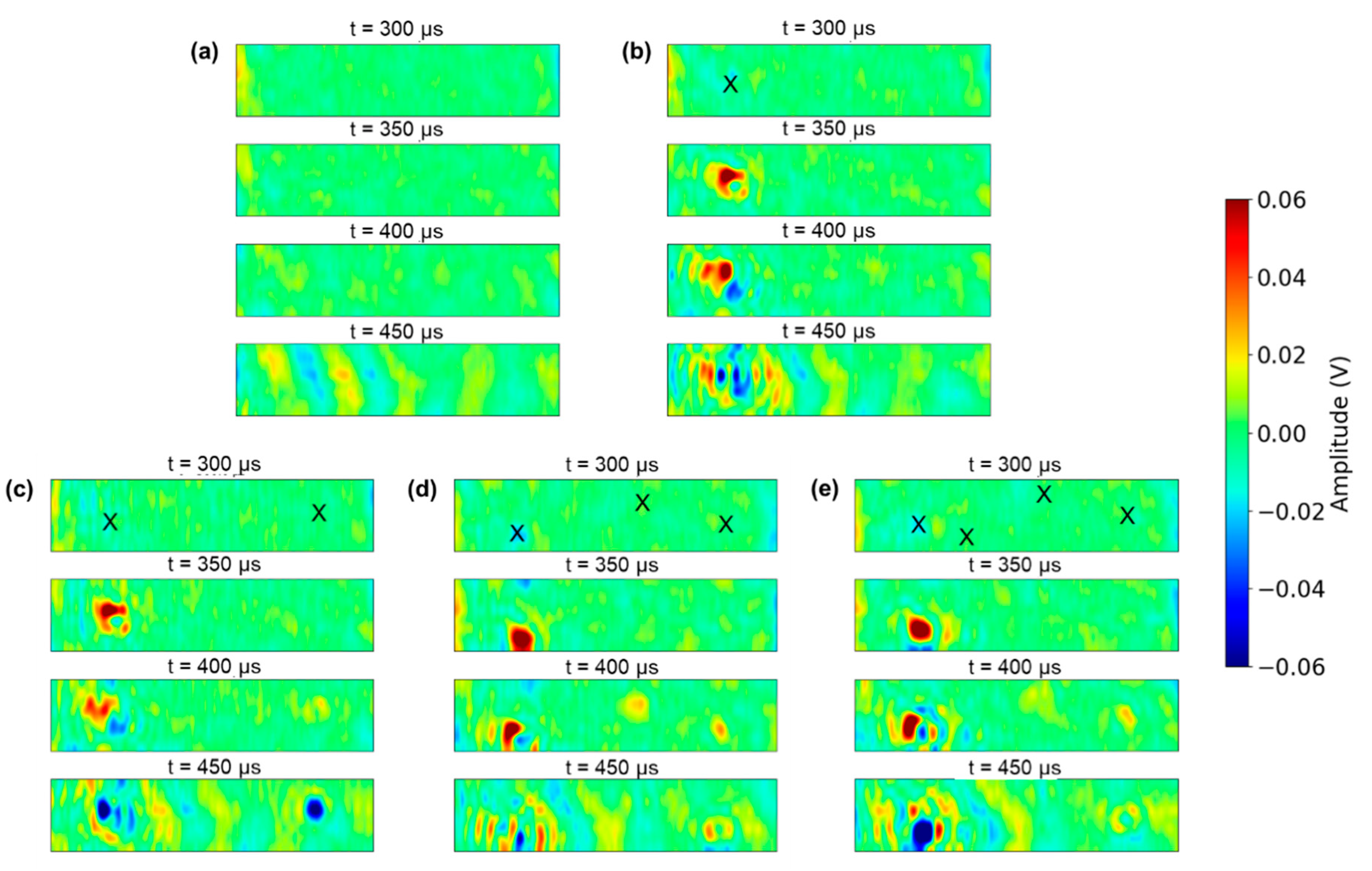
3.1. Ultrasonic Wavefield Data

An example time domain ultrasonic surface wave signal collected from the pristine concrete sample case is shown in Figure 3, which reveals suitably high signal-to-noise level. Measured ultrasonic time-space domain surface wave data for all the sample cases are shown in Figure 4. The total time required to acquire each wavefield data set was 5.6 min when using the following data acquisition parameters: 25 time averages per signal and an 80 ms pulse repetition interval. Although not presented nor discussed in this paper, the wavefield data acquisition time can be significantly reduced using a compressed sensing approach [18,20]. Wavefield snapshots at four time instances are shown for each wavefield data set, and the wavefield images each represent a 250 mm × 49 mm scan area. The locations of impact damage points are indicated as markers (‘X’) within the scan area for each sample case. In the figure, propagation of incident surface waves and scattered wavefields nearby impact damage locations are seen. In Case 0 (pristine concrete) seen in Figure 4a, forward propagating surface waves are the dominant wave components. Cases 1 to 4, seen in Figure 4b–e, show disruption to the forward propagating wavefield nearby the impact damage locations.
To better understand the scattered wavefields set up by impact damage, f-k domain signal analyses were carried out. The 3-D FTs of the ultrasonic wavefield data sets were computed using Equation (1). The f-k domain magnitude spectrum for each sample case was then normalized with respect to its maximum spectral magnitude. Figure 5 shows normalized f-kx-ky magnitude spectra for the wavefield data seen in Figure 4, where kx and ky are wavenumbers in horizontal and vertical directions, respectively. For visualization purposes, only spectra at the center frequency of excitation (43 kHz) are shown. The pristine concrete sample case (Case 0) seen in Figure 5a, mostly shows forward propagating surface wave components (indicated as ‘FP’) on the positive kx side. The damaged concrete samples cases (Cases 1 to 4 seen in Figure 5b–e) exhibit broadened magnitude spectra, with higher spectral energy outside the major (forward propagating) wavenumber band than for the pristine concrete case. The ultrasonic wavefield data and the corresponding f-k magnitude spectra demonstrate that impact damage in concrete sets up wavefields that exhibit wavenumber broadening. We presume that the wavenumber broadening is caused by surface wave scatter set up by the cracked damaged regions in the concrete.

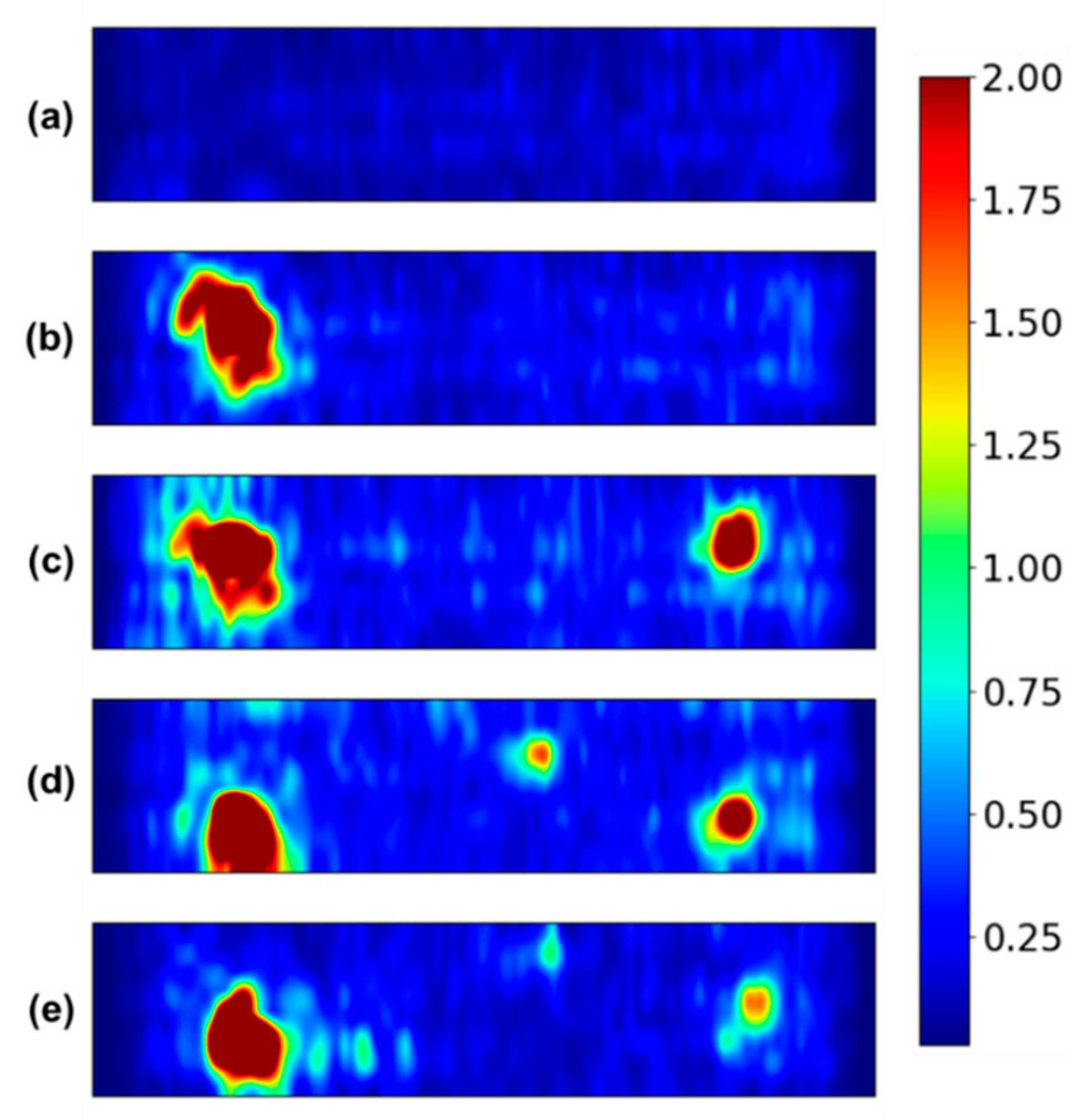
3.2. Concrete Damage Visualization

The complete wavefield data processing approach described in Section 2.3 was applied to the measured time-space wavefield data shown in Figure 4. Figure 6a,b show the filtering masks used to extract forward propagating surface waves (MFP) and non-propagating oscillatory fields (MNPO), respectively. Each mask is defined in f-kx-ky (3-D), but in the figure it is shown in kx-ky (2-D) at f = 43 kHz for visualization purposes. In the figures, white and black colors represent complete pass and reject of the masking function, respectively. Assuming that the majority of the wave components propagating in the pristine concrete sample takes the form of forward propagating surface waves, MFP shown in Figure 6a is defined as
M F P ( f , k x , k y ) = { 1 if   | S ¯ p ( f , k x , k y ) | > 0.05   max ( | S ¯ p | ) 0 otherwise ,
where | S ¯ p | is the f-k magnitude spectrum (3-D) of the wavefield from the pristine concrete sample. Here, the f-k region having magnitude greater than 5% of max ( | S ¯ p | ) is assumed to capture most of the forward propagating surface wave energy. Then, MNPO shown in Figure 6b is defined to suppress forward propagating and back-scattered surface waves using
M N P O ( f , k x , k y ) = { 1 M F P ( f , k x , k y ) if   k x > 0 1 M B S ( f , k x , k y ) if   k x 0 ,
where MBS is the f-k domain mask to extract back-scattered surface waves that is obtained by flipping MFP with respect to zero-kx line (kx = 0). Although back-scattered surface waves can indicate presence of damage, we suppress them to extract non-propagating wave components that can have higher damage localization capability.
The extracted forward propagating wavefields using MFP (Figure 6a) for all the concrete sample cases are shown in Figure 7, and the extracted non-propagating oscillatory fields using MNPO (Figure 6b) in Figure 8. The extracted forward propagating surface waves for all the concrete sample cases show similarity in amplitudes and geometric patterns, demonstrating insensitivity of forward propagating components to concrete damage. A significant distinction between each sample case is observed from the extracted non-propagating oscillatory fields however, as shown in Figure 8. The pristine concrete sample (Case 0) case, shown in Figure 8a, indicates a very small amount of non-propagating wave energy throughout the scanned region. The damaged sample cases (Cases 1 to 4), shown in Figure 8b–e, exhibit non-propagating wave components with high oscillatory energies nearby the impact locations.
Normalized non-propagating wave energy maps, E N P O N ( x , y ) , for all the tested concrete sample cases are shown in Figure 9. As observed from the extracted non-propagating oscillatory fields in Figure 8, the damaged sample cases (Figure 9b–e) show higher E N P O N values nearby the impact locations, while the pristine sample case (Figure 9) shows negligible E N P O N values throughout the scanned area.

4. Discussion

The measured ultrasonic wavefield data seen in Figure 4 demonstrate that near-surface concrete damage introduced by mechanical impacts set up distinct non-propagating oscillatory fields nearby the impact locations. Such non-propagating oscillatory fields can be considered multiply reflected wave events from multiple scatterers (e.g., cracks) that are densely gathered within a localized region of a medium [19]. Considering the strong oscillatory responses observed nearby the impact locations, especially D1 and D2, the damage is presumed to be present in the form of multiple scatterers (presumably cracks) densely gathered nearby the impact points rather than by surface pits. If the impact damage was present in the form of surface pits, the scattered wavefields would have been in the form of propagating waves (e.g., back-scattered surface waves or radiated surface waves from the pits).
The localized nature of the non-propagating oscillatory fields causes magnitude spectra broadening in the wavenumber domain as shown in Figure 5. Because of their localized nature, the non-propagating oscillatory fields enable localization (or visualization) of concrete damage within a scan area. The normalized non-propagating wave energy maps shown in Figure 9 demonstrate the potential of the proposed approach to detect and to visualize near-surface concrete damage.
We assert that the presented approach is insensitive to small variations of signal processing parameters, in particular the nature of the filtering masks MFP and MNPO. As long as MFP suitably covers the wavenumber range where most forward propagating wave components are present, the filtered responses and the corresponding damage visualization maps should not vary significantly.
In the experiments, we introduced near-surface concrete damage using mechanical impacts. Impact-based damage is suitable for laboratory investigations. However, these artificial damage types differ from real-world concrete damage (e.g., those caused by deterioration mechanisms) in damage morphology, geometric connectivity, and dimension. Such discrepancies in geometric features of damage may cause important discrepancies in scattered wavefields. Further research on ultrasonic wavefield imaging applied to damaged concrete by realistic deterioration mechanism is needed. We are currently addressing this issue by conducting experiments on concrete samples subjected to realistic damage-promoting environments including that caused by alkali-silica reaction and freezing/thawing cycles.
The wavefield imaging hardware presented in this study should be further improved for industrial or field applications. Also, quantitative damage characterization (e.g., crack sizing) should be carried out for in-depth characterization of detected damage. We set these topics as our future work.

5. Conclusions

This paper describes work to visualize near-surface concrete damage using a contactless ultrasonic wavefield imaging technique. Based on the presented work, the following conclusion are drawn:
  • Near-surface concrete cracking damage introduced by mechanical impact scatter incident surface waves and set up distinct non-propagating oscillatory wavefields that exhibit broadened wavenumbers;
  • The proposed f-k domain wavefield data processing approach can extract non-propagating oscillatory field contributions to the wavefields caused by near-surface damage; and
  • An extracted non-propagating wave energy map enables visualization and location of near-surface damage in concrete.

Author Contributions

H.S. and J.S.P. designed the study. H.S. carried out experiments, analyzed the collected data, and wrote the manuscript draft. J.S.P. acquired the funding, supervised the study, reviewed and improved the manuscript draft.

Funding

This research was funded by the Integrated Research Program-Nuclear Energy University Program of U.S. Department of Energy under grant number DE-NE0008266.

Conflicts of Interest

The authors declare no conflict of interest.

References

  1. Michaels, J.E. Ultrasonic wavefield imaging: Research tool or emerging NDE method? AIP Conf. Proc. 2017, 1806, 020001. [Google Scholar]
  2. Ruzzene, M. Frequency-wavenumber domain filtering for improved damage visualization. Smart Mater. Struct. 2007, 16, 2116–2129. [Google Scholar] [CrossRef]
  3. Yu, L.; Tian, Z.; Leckey, C.A. Crack imaging and quantification in aluminum plates with guided wave wavenumber analysis methods. Ultrasonics 2015, 62, 203–212. [Google Scholar] [CrossRef] [PubMed]
  4. Mesnil, O.; Yan, H.; Ruzzene, M.; Paynabar, K. Fast wavenumber measurement for accurate and automatic location and quantification of defect in composite. Struct. Health Monit. 2016, 15, 223–234. [Google Scholar] [CrossRef]
  5. Michaels, T.E.; Michaels, J.E.; Ruzzene, M. Frequency-wavenumber domain analysis of guided wavefields. Ultrasonics 2011, 51, 452–466. [Google Scholar] [CrossRef] [PubMed]
  6. Flynn, E.B.; Chong, S.Y.; Jarmer, G.J.; Lee, J.R. Structural imaging through local wavenumber estimation of guided waves. Ndt E Int. 2013, 59, 1–10. [Google Scholar] [CrossRef]
  7. Park, B.; An, Y.K.; Sohn, H. Visualization of hidden delamination and debonding in composites through noncontact laser ultrasonic scanning. Compos. Sci. Technol. 2014, 100, 10–18. [Google Scholar] [CrossRef]
  8. Lee, J.R.; Cho, C.M.; Park, C.Y.; Truong, C.T.; Shin, H.J.; Jeong, H.; Flynn, E.B. Spar disbond visualization in in-service composite UAV with ultrasonic propagation imager. Aerosp. Sci. Technol. 2015, 45, 180–185. [Google Scholar] [CrossRef]
  9. An, Y.K.; Park, B.; Sohn, H. Complete noncontact laser ultrasonic imaging for automated crack visualization in a plate. Smart Mater. Struct. 2013, 22, 025022. [Google Scholar] [CrossRef]
  10. Kudela, P.; Radzieński, M.; Ostachowicz, W. Identification of cracks in thin-walled structures by means of wavenumber filtering. Mech. Syst. Signal Process. 2015, 50, 456–466. [Google Scholar] [CrossRef]
  11. Yu, L.; Tian, Z.; Li, X.; Zhu, R.; Huang, G. Core–skin debonding detection in honeycomb sandwich structures through guided wave wavefield analysis. J. Intell. Mater. Syst. Struct. 2018, 30, 1306–1317. [Google Scholar] [CrossRef]
  12. Algernon, D.; Grafe, B.; Mielentz, F.; Köhler, B.; Schubert, F. Imaging of the elastic wave propagation in concrete using scanning techniques: Application for impact-echo and ultrasonic echo methods. J. Nondestruct. Eval. 2008, 27, 83–97. [Google Scholar] [CrossRef]
  13. Aggelis, D.G.; Shiotani, T. Experimental study of surface wave propagation in strongly heterogeneous media. J. Acoust. Soc. Am. 2007, 122, EL151–EL157. [Google Scholar] [CrossRef] [PubMed]
  14. Chekroun, M.; Le Marrec, L.; Abraham, O.; Durand, O.; Villain, G. Analysis of coherent surface wave dispersion and attenuation for non-destructive testing of concrete. Ultrasonics 2009, 49, 743–751. [Google Scholar] [CrossRef] [PubMed] [Green Version]
  15. Abraham, O.; Piwakowski, B.; Villain, G.; Durand, O. Non-contact, automated surface wave measurements for the mechanical characterisation of concrete. Constr. Build. Mater. 2012, 37, 904–915. [Google Scholar] [CrossRef]
  16. Kaczmarek, M.; Piwakowski, B.; Drelich, R. Noncontact Ultrasonic Nondestructive Techniques: State of the Art and Their Use in Civil Engineering. J. Infrastruct. Syst. 2016, 23, B4016003. [Google Scholar] [CrossRef]
  17. Song, H.; Popovics, J.S.; Park, J. Development of an automated contactless ultrasonic scanning measurement system for wavefield imaging of concrete elements. In Proceedings of the IEEE International Ultrasonics Symposium (IUS), Washington, DC, USA, 6–9 September 2017. [Google Scholar]
  18. Song, H.; Park, J.; Popovics, J.S. Contactless ultrasonic wavefield imaging of concrete using a MEMS microphone array and compressed sensing. Mech. Syst. Signal Process. 2019. submitted. [Google Scholar]
  19. Song, H.; Popovics, J.S. Extracting non-propagating oscillatory fields in concrete to detect distributed cracking. J. Acoust. Soc. Am. 2019. submitted, under review. [Google Scholar]
  20. Mesnil, O.; Ruzzene, M. Sparse wavefield reconstruction and source detection using Compressed Sensing. Ultrasonics 2016, 67, 94–104. [Google Scholar] [CrossRef] [PubMed]
Figure 1. The contactless scanning ultrasound measurement hardware (left) and the concrete sample (right) that shows impact damage locations; ultrasonic scan area indicated by red box. Impact damage points were introduced sequentially from the position D1 to D4.
Applsci 09 03005 g001
Figure 2. An overview of the proposed f-k domain wavefield data processing approach.
Applsci 09 03005 g002
Figure 3. Example time domain surface wave signal collected from the pristine sample (Case 0).
Applsci 09 03005 g003
Figure 4. Measured time-space domain wavefield data: (a) Case 0 (pristine), (b) Case 1 (D1 only), (c) Case 2 (D1 and D2), (d) Case 3 (D1 to D3) and (e) Case 4 (D1 to D4). The wavefield images each represent a 250 mm (horizontal) × 49 mm (vertical) scan area. ‘X’ indicates an impact damage location.
Applsci 09 03005 g004
Figure 5. Normalized f-k (f-kx-ky) domain magnitude spectra of the wavefield data at the center frequency of excitation (f = 43 kHz): (a) Case 0 (pristine), (b) Case 1 (D1 only), (c) Case 2 (D1 and D2), (d) Case 3 (D1 to D3) and (e) Case 4 (D1 to D4). The color bar indicates normalized spectral amplitude.
Applsci 09 03005 g005
Figure 6. Filtering masks to extract (a) forward propagating surface waves (MFP) and (b) non-propagating oscillatory fields (MNPO). In the images, the white color represents complete pass and the black color complete reject of the masking function. Each mask is defined in f-kx-ky (3-D), but here is shown in kx-ky (2-D) at f = 43 kHz for visualization purposes.
Applsci 09 03005 g006
Figure 7. Extracted forward propagating surface waves: (a) Case 0 (pristine), (b) Case 1 (D1 only), (c) Case 2 (D1 and D2), (d) Case 3 (D1 to D3) and (e) Case 4 (D1 to D4). The wavefield images each represent a 250 mm (horizontal) × 49 mm (vertical) scan area. ‘X’ indicates impact damage locations.
Applsci 09 03005 g007
Figure 8. Extracted non-propagating oscillatory fields: (a) Case 0 (pristine), (b) Case 1 (D1 only), (c) Case 2 (D1 and D2), (d) Case 3 (D1 to D3) and (e) Case 4 (D1 to D4). The wavefield images each represent a 250 mm (horizontal) × 49 mm (vertical) scan area. ‘X’ indicates impact damage locations.
Applsci 09 03005 g008
Figure 9. Normalized non-propagating wave energy maps E N P O N ( x , y ) : (a) Case 0 (pristine), (b) Case 1 (D1 only), (c) Case 2 (D1 and D2), (d) Case 3 (D1 to D3) and (e) Case 4 (D1 to D4). Each scan area represents a 250 mm (horizontal) × 49 mm (vertical) scan area.
Applsci 09 03005 g009
Table 1. Mixture design proportions for the concrete sample.
ContentsUnit Weight [kg/m3]
Cement406.5
Water192.7
Fly ash71.7
Coarse aggregate *953.5
Fine aggregate663.5
* The nominal maximum aggregate size is 25.4 mm.
Table 2. The pristine and damaged sample cases considered for testing.
CaseThe Number of Impact Damage Points
00 (Pristine)
11 (D1 only)
22 (D1 & D2)
33 (D1 to D3)
44 (D1 to D4)

