Redundancy Removed Dual-Tree Discrete Wavelet Transform to Construct Compact Representations for Automated Seizure Detection

Abstract

With the development of pervasive sensing and machine learning technologies, automated epileptic seizure detection based on electroencephalogram (EEG) signals has provided tremendous support for the lives of epileptic patients. Discrete wavelet transform (DWT) is an effective method for time-frequency analysis of EEG and has been used for seizure detection in daily healthcare monitoring systems. However, the shift variance, the lack of directionality and the substantial aliasing, limit the effects of DWT in some applications. Dual-tree discrete wavelet transform (DTDWT) can overcome those drawbacks but may increase information redundancy. For classification tasks with small dataset sizes, such redundancy can greatly reduce learning efficiency and model performance. In this work, we proposed a novel redundancy removed DTDWT (RR-DTDWT) framework for automated seizure detection. Energy and modified multi-scale entropy (MMSE) features in a dual tree wavelet domain were extracted to construct a complete picture of mental states. To the best of our knowledge, this is the first study to employ MMSE as an indicator of epileptic seizures. Moreover, a compact EEG representation can be obtained after removing useless information redundancy (redundancy between wavelet trees, adjacent channels and entropy scales) by a general auto-weighted feature selection framework via global redundancy minimization (AGRM). Through validation on Bonn and CHB-MIT databases, the proposed RR-DTDWT method can achieve better performance than previous studies.

1. Introduction

Epilepsy is a functional disorder caused by paroxysmal abnormal discharge of brain cells. According to the World Health Organization, about 50 million patients worldwide of all ages are suffering from epilepsy [1]. Conventional manual seizure inspection of long-term EEG monitors is time-consuming. With the rapid development of pervasive sensing in daily healthcare system and machine learning technologies, computer-aided diagnosis mechanisms, such as automated seizure detection based on electroencephalogram (EEG), provides tremendous support for a patient’s health and quality of life [2]. Such automated seizure detectors can trigger alarm when users are or will possibly be in a state of seizure. So far, algorithms for automated epileptic seizure detection proposed in most studies consist of three parts: (1) signal domain transformation, such as frequency domain via Fourier transform [3], wavelet time-frequency domain via discrete wavelet transform (DWT) [4,5], weighted and specific shapes via Hermite transformation [6] or original domain without transformation [7]; (2) feature extraction in the target domain, such as energy features [8] and complexity features [9]; and (3) machine learning based classification using a support vector machine (SVM) [10], k-nearest neighbor (KNN) [11] or artificial neural network (ANN) [12]. However, all the aforementioned three parts have shown limitations in some application scenarios, which are discussed in the following paragraphs separately.

For signal domain transformation, in spite of the many transformed domains explored for automated epileptic seizure detection, the most discriminative information resides in the time-frequency domain due to the evident transient characteristics and rich frequency components of epilepsy EEG. Accordingly, discrete wavelet transform (DWT) [4,5] has been widely applied in EEG based epileptic seizure detection applications because it can represent both the time and frequency characteristics of EEG signals. However, some drawbacks of DWT, such as shift variance, lack of directionality and the oscillation attribute of DWT coefficients [13], limit its effectiveness in some applications. Moreover, the iterated downsampling operations during wavelet decomposition may introduce severe aliasing [13]. Such aliasing can lead to information loss of original signals. Dual tree DWT (DTDWT) [13] can overcome the aforementioned drawbacks of DWT at the cost of increasing information redundancy (a $2^d$ redundancy factor for d-dimensional signals). But large redundancy may greatly reduce learning efficiency, which in turn weakens the performance of the trained models.

For feature extraction in the target domain, complexity features [9] have received a great deal of attention in the biomedical signal processing field in recent years. To measure the complexity property of EEG signals during epileptic seizures, entropy-based features have been widely used, such as sample entropy [9], fuzzy entropy [10], approximate entropy [14], permutation entropy [15] and distribution entropy [9]. All these entropy indicators listed above measure EEG complexity on a single scale. The single scale complexity measure may fail to quantify the underlying dynamics of the extremely complex physiological signals. Therefore, multi-scale entropy (MSE) was proposed [16]. However, the coarse-graining procedure during MSE computation can shorten the length of time sequence but a precise entropy relies heavily on a longer sequence length.

For machine learning based classification between normal (or interictal) and ictal seizure EEG, as mentioned earlier, large redundancy may greatly reduce the learning efficiency and increase model complexity. Epileptic seizure detection is a pattern recognition task with a small dataset size due to the scarcity of ictal seizure EEG. With only a small database available for model training, the large amount of redundancy in the seizure detection scenario will especially weaken the model performance. Due to the huge cost of data collection and data labeling, another alternative solution is to construct a compact data representation, reducing the dependence on data volume. Therefore, redundancy removal is crucial. Some classical redundancy reduction methods, such as principal component analysis (PCA) [17] do not take feature separability into consideration. For a pattern recognition problem, the high feature separability and low redundancy are both important.

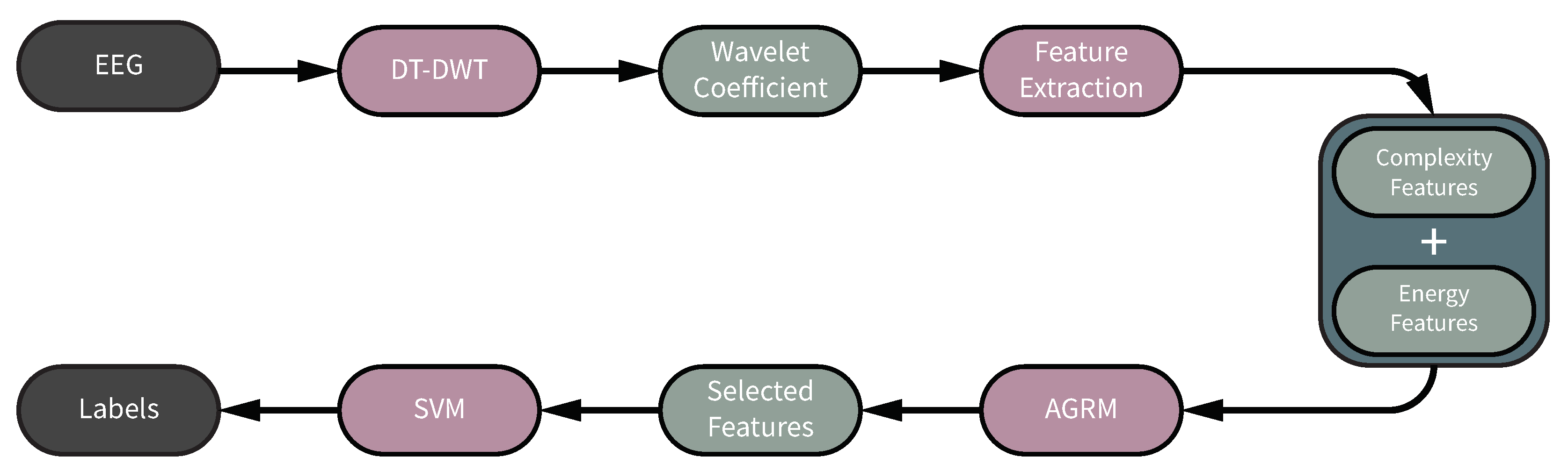
To address the aforementioned issues, we propose a novel framework of redundancy removed DTDWT (RR-DTDWT) to reduce global redundancy introduced by DTDWT and achieve a compact signal representation through low-redundancy features in the wavelet domain. First, DTDWT was employed to represent EEG signals in dural tree wavelet domain and at the same time, to overcome the drawbacks of DWT at the cost of increasing information redundancy. Then, energy and complexity features were both extracted for classification in our method. The energy features refer to the mean absolute values and variance-like statistic metrics. To measure the complexity property of EEG signals and reduce the influence of the short length of time sequence on entropy calculation, we used modified multi-scale entropy (MMSE) [18] to represent the complexity of EEG signals. MMSE can overcome the shortcoming of MSE by replacing the coarse-graining procedure with a moving-average procedure. To the best of our knowledge, this is the first study to evaluate the effectiveness of MMSE for seizure detection. We constructed a complete picture to represent mental electrophysiological activity in wavelet domain with both a wealth of useful information and redundancy. The redundancy in this work was introduced from three levels: (1) redundancy between adjacent EEG channels, (2) redundancy between dual wavelet trees and (3) redundancy between entropy in different scales. Therefore, in the next step, we aimed to minimize the global redundancy, and meanwhile retain the feature separability. In our work, auto-weighted feature selection via global redundancy minimization (AGRM) [19] was used to reduce the information redundancy. AGRM can take both feature redundancy and separability into account. Moreover, the optimization problem involved in AGRM is convex, so that a global optimum instead of local optimum can be obtained. In our work, a compact representation of the EEG signal can be obtained after removing information redundancy by AGRM. We validated the proposed RR-DTDWT framework on two benchmark databases (Bonn database and CHB-MIT database). The results on both databases demonstrate that RR-DTDWT can yield competitive results compared with previous studies.

2. Methodologies

The proposed RR-DTDWT consists of four parts; namely, DTDWT-based signal domain transformation, feature extraction, AGRM-based feature selection and SVM-based classification. The framework of the proposed method is shown in Figure 1. The principles of the four parts are given separately in the following subsections.

2.1. Dual-Tree Discrete Wavelet Transform (DTDWT)

DWT employs analysis filters to decompose signals into approximation components and detail components. Then 1/2 downsampling was applied to obtain the approximation coefficients and detail coefficients. The downsampling procedure may introduce severe aliasing, leading to distortion which may reduce the ability of wavelet coefficients to characterize the original signals. DTDWT is an enhancement of DWT which can overcome the above mentioned drawbacks. The flow chart of DTDWT is shown in Figure 2. As shown in Figure 2, DTDWT employs two wavelet trees for signal decomposition. For the first level decomposition, if the delay between two wavelet trees equals to the sampling interval, then the sample value discarded during the downsampling operation of the 1st wavelet tree is exactly the reserved one of the 2nd wavelet tree (equivalent to no downsampling operation). For decomposition in a higher level, alternate odd and even-length linear phase filters are utilized in DTDWT. However, the use of alternate odd/even filter approach is impractical in some scenarios. Therefore, a Q-shift [20] dual tree structure was proposed so that all filters beyond level 1 decomposition were of even-length. In our work, the 10-tap Q-shift filter was selected, which has been proven effective and is the common choice in many applications of DTDWT [21,22].

Through DTDWT (Figure 2), we can obtain 14 coefficient sets (2 sets of approximation coefficients: $A_{T1L6}$, $A_{T2L6}$; 12 sets of detail coefficients: $D_{T1L1}$, $D_{T2L1}$, $D_{T1L2}$, $D_{T2L2}$, ... , $D_{T1L6}$ and $D_{T2L6}$) for each EEG channel. Complexity and energy features were extracted directly from these wavelet coefficient sets.

2.2. Feature Extraction

2.2.1. Sample Entropy

Sample Entropy [23] was introduced for time-sequence analysis, complexity measurement in particular, which has been applied in physiological signal analysis [9]. For discrete time sequence $X=\left\{x\right(1),x(2),\dots ,x(N\left)\right\}$, the sample entropy can be calculated as follows:

(1) 

Construct a set of m-length vector series $\{X_m\left(1\right)$, $X_m\left(2\right)$, ... , $X_m(N-m+1)\}$, where $X_m\left(i\right)=\{x\left(i\right),x(i+1),\dots ,x(i+m-1\}$, $1\le i\le N-m+1$.

(2) 

Define $d[X_m\left(i\right),X_m\left(j\right)]$ to be the distance between $X_m\left(i\right)$ and $X_m\left(j\right)$, which takes the following form.

$$d[X_m\left(i\right),X_m\left(j\right)]=\underset{k=0,1,\dots ,m-1}{max}|x(i+k)-x(j+k)|.$$

(1)

(3) 

For a given $X_m\left(i\right)$, assign $B_i$ to be the number of j which meets the following condition: $d[X_m\left(i\right),X_m\left(j\right)]\le r$ and $j\ne i$, where r is the tolerance parameter. Then, define:

$$B_i^m\left(r\right)=\frac{1}{N-m-1}{B}_i.$$

(2)

(4) 

Define $B^{\left(m\right)}\left(r\right)$ to be:

$$B^{\left(m\right)}\left(r\right)=\frac{1}{N-m}\sum _{i=1}^{N-m}{B}_i^m\left(r\right).$$

(3)

(5) 

Increase the length of vector series from m to $m+1$. Then repeat step (1) to (4) to obtain $B^{(m+1)}\left(r\right)$.

(6) 

The sample entropy of time sequence X is:

$$SameEn(m,r)=\underset{N\to \infty }{lim}-ln\left(\frac{B^{(m+1)}\left(r\right)}{B^{\left(m\right)}\left(r\right)}\right).$$

(4)

When N is a finite value, sample entropy can be estimated by the following formula:

$$SameEn(m,r)=-ln\left(\frac{B^{(m+1)}\left(r\right)}{B^{\left(m\right)}\left(r\right)}\right).$$

(5)

2.2.2. Multi-Scale Entropy

Sample entropy may fail to interpret the signal complexity in multiple time scales. MSE was, thus, proposed [16]. MSE accounts for complex dynamics of time sequence over multiple scales by introducing the coarse-graining process directly before entropy calculation. For discrete time sequence $X=\left\{x\right(1),x(2),\dots ,x(N\left)\right\}$, the coarse-grained time sequence $\left\{y^{\left(\tau \right)}\right\}$ can be calculated by the following formula:

$$y^{\left(\tau \right)}=\frac{1}{\tau }\sum _{i=(j-1)\tau +1}^{j\tau }x\left(i\right),1\le j\le \frac{N}{\tau },$$

(6)

where $\tau$ is the scale factor. Then, we can obtain the sample entropy of the coarse-grained time sequence $\left\{y^{\left(\tau \right)}\right\}$ as MSE in scale $\tau$.

2.2.3. Modified Multi-Scale Entropy

Although MSE can quantify complex dynamics of time sequence over multiple scales, there are still some limitations. Considering time sequence with a length of 100 points, MSE in scale 5 is calculated by only 20 coarse-grained points. However, a precise complexity analysis relies heavily on time sequence with sufficient samples. MMSE was proposed for complexity measurement of short-term time sequence [18] and has been applied for signal complexity analysis [24,25]. In this work, entropy features were extracted directly from wavelet coefficients. The iterated downsampling operations of DTDWT greatly reduce the lengths of coefficient sets in high level decomposition. Accordingly, MMSE is preferred rather than MSE to estimate complexity of short wavelet coefficients. For MMSE, the coarse-grained time sequence $\left\{y^{\left(\tau \right)}\left(j\right)\right\}$ is calculated through moving-average strategy as follows:

$$y^{\left(\tau \right)}\left(j\right)=\frac{1}{\tau }\sum _{i=j}^{j+\tau -1}x\left(i\right),1\le j\le N-\tau +1.$$

(7)

Instead of utilizing disjoint time window to divide original time sequence into coarse-grained sample points, for MMSE, an overlapping moving window was applied. Therefore, the length of coarse-grained time sequence increases from $N/\tau$ to $N-\tau +1$. According to previous study [26], $m=1$ or $m=2$ with r fixed at a value between 0.1 and 0.25 of the standard deviation (STD) of time sequence was suggested. Many applications of sample entropy selected parameters following this criterion [27]. Specifically, $r=0.15\times STD$ was selected in [28]. In our method, $m=2$, $r=0.15\times STD$ and $\tau =\{1,2,3,4,5\}$ (5 scales) were selected for MMSE calculation.

2.2.4. Energy Features

Energy features, namely, variance and mean absolute values of wavelet coefficient sets, were also extracted for classification, as a complement of the complexity features.

2.3. Feature Selection Based on Auto-Weighted Feature Selection via Global Redundancy Minimization (AGRM) Algorithm

The extracted features in above procedures contain huge amounts of redundant information. For pattern recognition problems with small dataset size, epileptic seizure detection for example, such redundancy may greatly reduce learning efficiency and model performance. In this section, we introduce the principle of a latest redundancy removal algorithm, namely, AGRM, which has been proven quite effective in the image processing field. Traditional redundancy removal algorithms only focus on minimizing feature redundancy but ignore feature separability. For AGRM, feature redundancy and separability are both taken into consideration at the same time. We denote the feature matrix as $F\in {\mathbb{R}}^{n\times d}$, where rows of F correspond to observations and columns to features. Each column $f_i$ ($i\in \{1,2,\dots ,d\}$) has been normalized by Z-score. The objective function of AGRM takes the following form,

$$\begin{array}{c}\hfill \underset{z,\lambda }{min}{\lambda }^2{z}^{T}Az-\lambda z^{T}s\\ \hfill s.t.z^T\mathbf{1}=1,z\ge 0,\end{array}$$

(8)

where $\mathbf{1}={(1,1,\dots ,1)}^T$ and $z\in {\mathbb{R}}^{d\times 1}$ refer to the final feature score obtained by AGRM so that the top ranking features are selected to represent the original signals. Matrix $A\in {\mathbb{R}}^{d\times d}$ in objective function (8) denotes pair-wise feature redundancy, where $A_{i,j}={\left(\frac{f_i^T{f}_j}{\parallel f_i\parallel \parallel f_j\parallel }\right)}^2$. Besides, $s\in {\mathbb{R}}^{d\times 1}$ refers to another input feature score to be jointly taken into account. In this work, s denotes the Fisher score of original features. We denote ${\mu }_i$ as the mean value of the ith feature of all EEG segments. Similarly, ${\mu }_i^k$ is the mean value of the ith feature of segments in class k. Given a feature $f_i$ in c known classes, with segment ID j in a specific class, Fisher score s can be computed as Equation (9).

$$s\left(i\right)=\frac{S_B}{S_W}=\frac{{\sum }_{k=1}^c\frac{n_k}{n}{({\mu }_i^k-{\mu }_i)}^2}{\frac{1}{n}{\sum }_{k=1}^c{\sum }_{j=1}^{n_k}{(f_{i;j}-{\mu }_i^k)}^2}.$$

(9)

In Equation (9), $S_B$ and $S_W$ denote feature distance between and within class respectively. Therefore, a higher Fisher score contributes to higher feature separability. The first term $z^{T}Az$ in (8) is the global redundancy of extracted features. The second term $z^{T}s$ in (8) denotes feature separability. And $\lambda$ acts as a trade-off parameter between the two terms, which comes to convergence automatically in optimization procedure. Obviously, by minimizing the objective function (8), feature redundancy is minimized while feature separability is maximized. The optimization problem of AGRM has been proven convex [19], so a global optimum can be achieved. The optimal z and $\lambda$ can be obtained by general augmented Lagrangian multiplier (ALM) method given by [19]. Here, we give a brief description of optimization procedure:

(1) 

Given input A and s, initialize $z=\frac{1}{d}\mathbf{1}$, $\rho >1$, $\mu$ and $\beta$.

(2) 

Unless $\lambda$ converges, repeat step (3).

(3) 

Compute $\lambda =\frac{z^{T}s}{2z^{T}Az}$ and update z by repeating step (4) until z converges.

(4) 

Update $v=z+\frac{s+\beta -\lambda Az}{\mu }$. Compute z by step (5). Update $\beta =\beta +\mu (z-v)$. Update $\mu =\rho \mu$.

(5) 

Compute $m=v-\frac{1}{\mu }(\beta +\lambda A^{T}v)$. Compute $g=m-\frac{{\mathbf{11}}^T}{d}m+\frac{1}{d}\mathbf{1}$. Use Newton’s method to obtain root ${\overline{\eta }}^{\ast }$ of equation ${\overline{\eta }}^{\ast }=\frac{1}{d}{\sum }_{t=1}^d{\left({\overline{\eta }}^{\ast }-g\left(t\right)\right)}_{+}$, where ${\left(x\right)}_{+}=max(x,0)$. For $\forall i$, the optimal $z^{\ast }\left(i\right)={\left(g\left(i\right)-{\overline{\eta }}^{\ast }\right)}_{+}$.

Following the optimization procedure above, feature scores z can be obtained. The leading features with higher scores are picked out to represent original data with minimal redundancy.

2.4. Classification with the Support Vector Machine

The SVM is a machine learning algorithm based on the structural risk minimization principle [29]. SVM has achieved great performance in many pattern recognition based advanced technologies, such as the human–machine interface based on muscle activity classification [30], the brain–computer interface based on mental state classification [31] and the engine control system based on fault diagnosis [32]. The principle of SVM is introduced in brief.

Given input feature vectors $x=\{x_i,i=1,2,\dots ,N\}$ and the corresponding labels $y=\{y_i,i=1,2,\dots ,N\}$, where $x_i\in {\mathbb{R}}^{d\times 1}$, d is the dimensionality of the feature space, N is the dataset size and $y=1$ or $y=-1$ refer to the two categories (normal or ictal in this work) to be classified. We define a function $f\left(x\right)$ taking the following form:

$$f\left(x\right)=w^{T}x+b,$$

(10)

where $w\in {\mathbb{R}}^{d\times 1}$. SVM aims to find the optimal function $f\left(x\right)$ to achieve $f\left(x_i\right)\ge 0$ for $y_i=1$ and $f\left(x_i\right)<0$ for $y_i=-1$ so that data of two classes in the high-dimensional feature space are separated by the optimal hyper-plane $w^{T}x+b=0$. To obtain the optimal hyper-plane as the classification boundary with the maximal separating margin between the two classes [33], mathematically, the objective function of SVM takes the following form:

$$\begin{array}{cc}\hfill & \underset{w}{min}\frac{1}{2}{w}^{T}w=\frac{1}{2}{\parallel w\parallel }^2\hfill \\ \hfill s.t.& w^T{x}_i+b\ge 1,if{y}_i=1\hfill \\ \hfill s.t.& w^T{x}_i+b\le -1,if{y}_i=-1.\hfill \end{array}$$

(11)

The constraints in Equation (11) can be rewritten in a compact form:

$$s.t.y_i(w^T{x}_i+b)\ge 1.$$

(12)

Because the training data may not be perfectly separated by the obtained hyper-plane, the slack variables ${\xi }_i$ were employed to relax the constraints in Equation (12):

$$s.t.y_i(w^T{x}_i+b)\ge 1-{\xi }_i.$$

(13)

The objective function (11) can be further rewritten to the following form which constitutes the structural risk [29]:

$$\underset{w,\xi }{min}\frac{1}{2}{\parallel w\parallel }^2+C\sum _{i=1}^N{\xi }_i.$$

(14)

The objective function (14) takes both the model complexity (the first term) and the training error (the second term) into consideration. The optimal solution of objective function (14) can be obtained through Lagrange multipliers [33].

3. Databases and Results

3.1. Databases

In this section, we give a description on the two benchmark databases utilized in this study.

3.1.1. Bonn Database

Bonn database built by Andrzejak et al. at Bonn University, Germany, contains artifact-free data collected from five healthy subjects and five epilepsy patients. The artifacts due to muscle activity and eye movements were pre-removed through visual examination. Two classification tasks were used to evaluate the effectiveness of our method: (1) normal EEG (set A) versus ictal EEG (set E); (2) interictal EEG (set C) versus ictal EEG (set E). Each set contained 100 single-channel EEG segments of 23.6 s duration. EEG data were acquired at a 173.61 Hz sampling rate using 12-bit resolution. For more details, please refer to [34].

In the preprocessing procedure, the single-channel EEG signal was normalized by Z-score. The normalized signals with zero-mean and one-standard deviation were prepared for subsequent feature extraction process.

In feature extraction procedure, due to the relatively low segment duration and sampling rate, the approximation and detail coefficient sets at the 6th decomposition level ($A_{T1L6}$, $D_{T1L6}$, $A_{T2L6}$ and $D_{T2L6}$) were of extremely short length (64 coefficients), which cannot support a reliable complexity analysis. MMSE features extracted from these four coefficient sets were excluded from the feature vector. Accordingly, a 50-dimensional MMSE feature vector was constructed (the remaining 10 coefficient sets × 5 entropy scales × 1 EEG channel). As for energy features, the variance and mean absolute value were extracted from each wavelet coefficient set, constructing a 28-dimensional energy feature vector (14 coefficient sets × 2 indicators × 1 EEG channels). In summary, a 78-dimensional feature vector was constructed for each EEG segment.

In the feature selection and classification procedure, we employed the “leave-one-out” cross-validation strategy. Because EEG data from all patients are mixed together in Bonn database, no patient label is available. Most studies in the literature also employed the cross-validation strategy on all data [6,35,36], which is consistent with our study. Considering that the dimensionality of original feature space is relatively low, all features with positive feature scores were retained while discarding those with zero scores (according to the last step of AGRM optimization procedure, the feature scores are non-negative values). We first held out one EEG segment as test data. All remaining data were allocated to training set, used for both AGRM-based feature score calculation and SVM model training. A label of “normal”, “interictal” or “ictal” for the held-out test data could be given by the trained SVM. We applied the same procedure to all EEG data so that all EEG segments were used to test algorithm performance. We employed sensitivity, specificity, precision, accuracy and F1 score as classification evaluation metrics.

3.1.2. CHB-MIT Database

CHB-MIT database published by Shoeb [37] contains long-term multi-channel EEG data of 24 epilepsy patients (1.5–22 years old) collected at the Children’s Hospital of Boston-Massachusetts Institute of Technology, with a 256 sampling rate and a 16-bit resolution. Data in CHB-MIT database were acquired continuously during long-term EEG monitoring with no signal processing performed after acquisition. The raw EEG data can better simulate a practical application scenario. The subset of each patient contains a varying number (between 9 and 42, 27.25 ± 9.68 on average) of .edf files. Generally, the digitized recordings in most files are one-hour long. The beginning and end time of each seizure ictal case has been labeled based on expert judgments. We divided the continuously recorded data into 30 s EEG segments. There are totally 198 seizure ictal cases in the database. Due to the non-uniform electrode distribution during data acquisition, 181 out of 198 seizures which shared common 23 channels were utilized for method validation. For each seizure ictal case, only one 30 s segment was used in our experiment to avoid the overestimation of algorithm performance due to the similarity among several segments in one seizure ictal case. Because of the scarcity of epilepsy ictal segments (181 segments), we randomly downsampled interictal EEG data to rebalance the ratio between ictal and interictal data (a final ratio of 1:3 in our validation experiment). To take the signal variability over time into consideration, the segmented interictal data were evenly distributed over different periods of time with no overlap. More details can be fetched in [37].

In preprocessing procedure, the EEG signal in each channel was normalized by Z-score. The normalized signals with zero-mean and one-standard deviation were prepared for subsequent feature extraction process.

In feature extraction procedure, MMSE features were first extracted from each coefficient set in each EEG channel, constructing a 1610-dimensional MMSE feature vector (14 coefficient sets × 5 entropy scales × 23 EEG channels). As for energy features, the variance and mean absolute value were extracted from each wavelet coefficient set, constructing a 644-dimensional energy feature vector (14 coefficient sets × 2 indicators × 23 EEG channels). In summary, a 2254-dimensional feature vector was constructed for each EEG segment.

In the feature selection and classification procedure, a specific classification model was developed for each patient. The “leave-one-out” cross-validation strategy was also applied to validate the proposed RR-DTDWT algorithm. We firstly held out one EEG segment as test data and all remaining EEG segments of all patients were allocated to the training set. Although a total number of 181 cases of seizure ictal EEG segments were contained in the experiment database, for each patient, very few cases of ictal seizures were available, which could not contribute to a precise feature correlation used for feature score calculation. Therefore, the AGRM-based feature score was pre-calculated using all EEG data in training set. The whole procedure was independent of the testing set. Due to the high dimensionality of original feature space, only the leading 50 features were selected. As for classification, due to the huge individual difference of EEG characteristics, the training data of the same patient as test data were used for SVM model training. The model trained in our work can be viewed as a patient-specific model, which is consistent with most automated seizure detection studies in the literature [7,38,39]. Similarly, we employed sensitivity, specificity, precision, accuracy and F1 score as classification evaluation metrics.

3.2. Qualitative Results

The pair-wise redundancy matrix of extracted features can help to better visualize the redundancy in the features extracted, as is shown in Figure 3. Here, we take CHB-MIT database as an example. According to the middle panel of Figure 3, it is obvious that energy-based features (mean absolute and variance) are highly correlated with each other, and the same is true for complexity-based features (MMSE). However, there is only a small amount of information redundancy between two kinds of features (energy-based and complexity-based features). According to the left panel of Figure 3, we can clearly see three bright diagonal lines. The middle diagonal line represents that each feature is highly correlated with itself. The lower left and upper right diagonal lines demonstrate the high redundancy between corresponding features extracted from two wavelet trees. According to the right panel of Figure 3, the periodic occurrence of the bright blocks indicates the high redundancy between adjacent EEG channels and between two wavelet trees. Moreover, the bright part of each block refers to the high redundancy between different entropy scales. In summary, from Figure 3, features extracted by DTDWT had high redundancy so an effective redundancy removal method was required to refine the extracted features.

The visualization of high-dimensional features (CHB-MIT database) by t-distributed stochastic neighbor embedding (t-SNE) [40] is shown in Figure 4. Although the epileptic seizure detector was trained specifically for each patient, here, we visualize data of all patients at the same time. Figure 4a represents visualization of original 2254-dimensional features with high redundancy. Obviously, ictal and interictal data is difficult to distinguish. Figure 4b represents visualization of 50-dimensional features after redundancy removal achieved by AGRM. Compared with scatter in Figure 4a, ictal and interictal data in Figure 4b are easier to classify, proving the effectiveness of redundancy removal.

3.3. Quantitative Results

3.3.1. Quantitative Results on Bonn Database

Algorithm comparisons for two different classification tasks, “normal versus ictal” and “interictal versus ictal,” on Bonn database, are shown in

Table 1. Performance of different methods on Bonn database (normal versus ictal).

Metrics	RR-DTDWT	RR-DWT	DTDWT	DWT	DTDWT + Fisher	DWT + Fisher
Sensitivity	100%	100%	100%	100%	100%	100%
Specificity	100%	99%	99%	99%	98%	98%
F1 Score	1	0.9950	0.9950	0.9950	0.9901	0.9901

RR-DWT: redundancy removed DWT; i.e., DWT-based features + AGRM. DWDWT + Fisher: DTDWT-based features + feature selection according to Fisher score. DWT + Fisher: DWT-based features + feature selection according to Fisher score.

and

Table 2. Performance of different methods on Bonn database (interictal versus ictal).

Metrics	RR-DTDWT	RR-DWT	DTDWT	DWT	DTDWT + Fisher	DWT + Fisher
Sensitivity	100%	100%	99%	99%	100%	100%
Specificity	100%	99%	97%	97%	98%	99%
F1 Score	1	0.9950	0.9802	0.9802	0.9901	0.9950

respectively. For both classification tasks, RR-DTDWT yielded an sensitivity and specificity of 100%. As a contrast, DTDWT, RR-DWT and DWT achieved a relatively lower performance. To avoid the performance bias caused by feature dimension, we also utilized Fisher score to reduce feature dimensionality (the same dimensionality as RR-DTDWT). As shown in Table 1 and Table 2, RR-DTDWT outperformed all other methods on the Bonn database.

3.3.2. Quantitative Results on CHB-MIT Database

We also present the algorithms’ performances on CHB-MIT database in

Table 3. Performance of different methods on CHB-MIT database.

Metrics	RR-DTDWT	RR-DWT	DTDWT	DWT	DTDWT + Fisher	DWT + Fisher
Sensitivity	96.69%	92.27%	92.82%	92.82%	93.92%	91.71%
Specificity	99.63%	98.35%	98.90%	99.27%	98.17%	98.17%
F1 Score	0.9813	0.9516	0.9573	0.9591	0.9596	0.9477

. Unlike DWT, the results of DTDWT and RR-DWT are almost the same (even slightly lower). This demonstrates that by simply extending DWT to DTDWT, the redundancy introduced limits the learning efficiency of model. Also, by directly applying AGRM to DWT-based features, some useful information may be lost. However, if we first employ DTDWT to complement the missing information of DWT, and then apply AGRM to reduce information redundancy, RR-DTDWT can achieve significantly higher results for all evaluation metrics. Similarly, we also employed Fisher score to reduce feature dimensionality (the same dimensionality as RR-DTDWT). RR-DTDWT still outperforms all other methods, as shown in Table 3.

4. Discussion

In this work, we proposed a RR-DTDWT framework for automated epileptic seizure detection. The propsed RR-DTDWT consists of four parts: (1) DTDWT-based signal domain transformation; (2) feature extraction; (3) feature selection and (4) classification. In the signal domain transformation part, the signal representation was obtained through DTDWT. DTDWT can reduce information loss during the iterated downsampling operation of DWT, at the cost of introducing information redundancy. In feature extraction part, energy and complexity features were extracted. MMSE was employed as an indicator of epileptic seizures for the first time. Then, AGRM-based feature selection could reduce the information redundancy and take feature separability into consideration at the same time. Finally, the label of each EEG segment was given by a patient-specific SVM classifier. In the following subsections, the comparison between our method and the ones from previous studies, the computational cost analysis and the limitations of our method are presented separately.

4.1. Comparison with Previous Studies

In this subsection, method comparison between the proposed RR-DTDWT algorithm and latest studies (after 2014) utilizing the same databases is presented.

4.1.1. Comparison with Previous Studies Based on Bonn Database

For Bonn database, method comparisons on two classification tasks, namely, “normal versus ictal” and “interictal versus ictal,” are presented in

Table 4. Comparison with previous studies on Bonn database (normal versus ictal).

Paper	Year	Methods	Sensitivity	Specificity	Precision	Accuracy	F1
[4]	2014	DWT + Fuzzy Approximate Entropy + SVM Classifier	100%	100%	100%	100%	1
[46]	2015	Discrete Short-Time Fourier Transform (DSTFT) + Multilayer Perceptron (MLP)	99.9%	99.6%	99.6%	99.8%	0.9975
[47]	2016	EMD-Based Temporal and Spectral Features + SVM	99%	-	-	-	-
[48]	2016	Weighted Permutation Entropy (WPE) + SVM	-	-	-	99.5%	-
[43]	2016	Dual-Tree Complex Wavelet Transformation + Normal Inverse Gaussian Parameters	100%	100%	100%	100%	1
[42]	2017	Wavelet Packet Transform (WPT) Based Entropy + ANN Classifier	99.40%	100%	100%	99.70%	0.9970
[41]	2017	Tunable-Q Wavelet Transform Based Multi-scale Entropy Features + SVM	100%	100%	100%	100%	1
[11]	2017	Genetic Algorithm-Based Frequency-Domain Feature Search (GAFDS) + KNN Classifier	-	-	-	99.5%	-
[49]	2018	Universum Twin Support Vector Machine (UTSVM)	-	-	-	99%	-
[50]	2018	A Novel Signal Modeling Approach Based on Discrete Cosine Transform and Hurst Exponent + SVM	95.40%	94.30%	94.36%	94.85%	0.9488
[51]	2018	Local Binary Pattern (LBP) Based on Wavelet Decomposition + SVM	-	-	-	99.63%	-
[35]	2018	Phase–Amplitude Cross-Frequency Coupling + SVM	100%	100%	100%	100%	1
[36]	2019	A Hybrid Model with Genetic Algorithm (GA) and Particle Swarm Optimization (PSO)	99.5%	99.25%	99.25%	99.38%	0.9938
[44]	2019	DWT + Random Forest Classifier	100%	91.66%	92.30%	99.95%	0.9600
[6]	2019	Hermite Transform + Permutation Entropy, Histogram Features and Statistical Features + SVM Classifier	-	-	-	99.5%	-
This Work	-	The Proposed RR-DTDWT (DTDWT + AGRM) + SVM	100%	100%	100%	100%	1

and

Table 5. Comparison with previous studies on Bonn database (interictal versus ictal).

Paper	Year	Methods	Sensitivity	Specificity	Precision	Accuracy	F1
[4]	2014	DWT + Fuzzy Approximate Entropy + SVM Classifier	99.3%	99.9%	99.9%	99.6%	0.9960
[46]	2015	Discrete Short-Time Fourier Transform (DSTFT) + Multilayer Perceptron (MLP)	99.3%	97.7%	97.74%	98.5%	0.9850
[43]	2016	Dual-Tree Complex Wavelet Transformation + Normal Inverse Gaussian Parameters	100%	100%	100%	100%	1
[42]	2017	Wavelet Packet Transform (WPT) Based Entropy + ANN Classifier	99.70%	100%	100%	99.85%	0.9985
[41]	2017	Tunable-Q Wavelet Transform Based Multi-scale Entropy Features + SVM	99%	100%	100%	99.5%	0.9950
[52]	2017	Weighted Complex Networks Based Community Structure Detection	99%	95%	95.19%	97%	0.9706
[53]	2017	Analytic Time-Frequency Flexible Wavelet Transform (ATF- FWT) + Least-Squares Support Vector Machine (LS-SVM) Classifier	-	-	-	99%	-
[54]	2018	Subpattern Based PCA and Cross-Subpattern Correlation-Based PCA + SVM Classifier	-	-	-	99.5%	-
[50]	2018	A Novel Signal Modeling Approach Based on Discrete Cosine Transform and Hurst Exponent + SVM	98%	97%	97.03%	97.50%	0.9751
[55]	2018	An Ensemble of Pyramidal One-Dimensional Convolutional Neural Network (P-1D-CNN) Models	-	-	-	98.5%	-
[35]	2018	Phase–Amplitude Cross-Frequency Coupling + SVM	100%	100%	100%	100%	1
[6]	2019	Hermite Transform + Permutation Entropy, Histogram Features and Statistical Features + SVM Classifier	-	-	-	98.5%	-
This Work	-	The Proposed RR-DTDWT (DTDWT + AGRM) + SVM	100%	100%	100%	100%	1

respectively. Because the data in Bonn database are balanced between each category, classification accuracy was expected to be a good metric to characterize method performance. Obviously, the proposed RR-DTDWT method outperformed most other latest methods, achieving an accuracy of 100% for both cases. As previously mentioned, Bonn database contains artifact-free EEG signals. The artifacts due to muscle activity and eye movements were pre-removed through visual examination. Accordingly, Bonn database cannot simulate the challenging practical application scenarios, although it can be utilized for method comparison. Some previous studies have also reported a 100% accuracy. For example, Battacharyya et al. [41] employed tunable-Q wavelet transform to develop a seizure detector which also achieved an accuracy of 100% for “normal versus ictal” problem. The model of Kumar et al. [4] can discriminate normal data from ictal data with a 100% accuracy and also discriminate interictal data from ictal data with a very low error rate. Methods proposed by Raghu et al. [42] yielded excellent performance for both classification tasks on Bonn database. Moreover, previous studies also proposed wavelet-based methods [43,44] and achieved a 100% or almost 100% classification accuracy. Akut et al. [45] proposed a wavelet-based deep learning approach in which no manual feature extraction was required. This method can achieve a high accuracy on small EEG database. All these studies made great contributions to the epilepsy monitoring field. Although our method achieved a 100% classification accuracy and outperformed most previous studies on Bonn database, its superior performance compared with other studies on the practical and challenging CHB-MIT database is described next.

4.1.2. Comparison with Previous Studies Based on CHB-MIT Database

For the CHB-MIT database, a method comparison is shown in

Table 6. Comparison with previous studies on the CHB-MIT database.

Paper	Year	Methods	Sensitivity	Specificity	FPR	Precision	Accuracy	F1
[10]	2015	Fuzzy Entropy + Kolmogorov-Smirnov Test + SVM.	98.27%	98.36%	2.03/h	98.36%	98.31%	0.9831
[12]	2016	Mel-Frequency Cepstral Coefficients (MFCCs) + Artificial Neural Network (ANN) Classifier.	98%	96%	4.8/h	96.08%	97%	0.9703
[39]	2016	Phase Space Representation + Linear Discriminant Analysis (LDA) + Naive Bayesian Classifier.	88.27%	93.21%	8.15/h	92.86%	93.11%	0.9051
[58]	2018	A Multi-Context Learning Approach by Incorporating a Feature Fusion Strategy.	98.65%	-	-	96.08%	95.71%	0.9725
[56]	2018	Short-Time Fourier Transform (STFT) + Convolutional Neural Networks (CNN).	81.2%	99.87%	0.16/h	99.84%	-	0.8956
[59]	2018	Deep CNN Using 1D and 2D Convolutional Layers to Extract Spatio-Temporal Correlation Features.	80.6%	91.7%	9.96/h	90.66%	85.6%	0.8534
[35]	2018	Phase–Amplitude Cross-Frequency Coupling + SVM	-	-	-	-	97.5%	-
[38]	2019	Nonlinear Dynamics and Nullclines + an Ensemble of Classifiers Network.	91.15%	95.16%	5.81/h	94.96%	95.11%	0.9301
[7]	2019	PCA + Poincare Sectioning + SVM + Naive Bayes Classifier.	95.7%	96.55%	4.14/h	96.52%	95.63%	0.9611
[60]	2019	Fuzzy-Rules-Based Sub-Sand Specific Features and Layered Directed Acyclic Graph SVM	99%	96%	4.8/h	96.12%	98%	0.9754
[57]	2019	DWT + Sigmoid Entropy +SVM	94.21%	-	-	-	94.38%	-
This Work	-	The Proposed RR-DTDWT (DTDWT + AGRM) + SVM	96.69%	99.63%	0.44/h	99.62%	98.89%	0.9813

. Different studies based on CHB-MIT database employed a wide variety of metric combinations to evaluate algorithm performance. For example, study [10,56] applied specificity and false positive rate (FPR) to characterize model performance respectively. To compare all methods consistently, we converted the two metrics into each other. For the proposed method, a specificity of 99.63% is equivalent to a false positive rate of 0.44/hour, under the assumption of 30 s EEG segments. The proposed RR-DTDWT can achieve a higher F1 score than most latest studies validated on CHB-MIT database. Only the F1 score of the detector developed by Xiang et al. [10] is slightly higher than ours. However, due to the long time EEG monitoring for epileptic seizure detection and the scarcity of ictal data, the acquired EEG data in real application scenarios characterize an extremely imbalanced ratio between ictal and interictal segments. Therefore, a high specificity in this application scenario may be equivalent to an unacceptable false alarm rate. For example, a detector with a seemingly high specificity of 95% is expected to trigger six false alarms per hour, which cannot be permitted in a practical application. Compared with the performance of [10], our detector approximately achieves a four fold reduction of FPR (from 2.03/h to 0.44/h) only at the cost of a slight reduction in sensitivity (from 98.27% to 96.69%). Based on the above discussions, our RR-DTDWT based detector is more suitable for realistic application scenarios compared with those listed in Table 6. Raghu et al. [57] also proposed an automated epileptic seizure detection method based on DWT and complexity measure via sigmoid entropy, achieving a sensitivity of 94.21% and an accuracy of 94.38%, which is less effective than our method. Previous studies such as [35] evaluated the performance of their method using both Bonn and CHB-MIT databases. Although their model has also shown a perfect performance on both of the two classification tasks (“normal versus ictal” and “interictal versus ictal”) on the Bonn dataset (see Table 4 and Table 5), its accuracy (97.5%) on more challenging CHB-MIT database shown in Table 6 is lower than ours (98.89%). Promisingly, our RR-DTDWT algorithm can further promote the development of automated seizure detection technology.

4.2. Computational Cost Analysis of the Proposed Redundancy Removed DTDWT (RR-DTDWT)

In this subsection, we analyze the computational cost of the proposed RR-DTDWT framework. In signal domain transformation part, DTDWT can be calculated with a computational cost of $O\left(N\right)$ [61], for a EEG segment with a length of N. In the energy-based feature extraction part, both mean absolute values and variance features can be calculated in $O\left(N\right)$ computational time. Complexity-based features such as sample entropy require $O\left(N^2\right)$ computation time. Using the fast computation algorithms, the computation time can be reduced to $O\left(N^{\frac{3}{2}}\right)$ [62]. Moreover, considering that biomedical signals are normally saved as digitized integer-type data, the computation time of sample entropy using a fast computation algorithm is only $O\left(N\right)$, or precisely, $O\left(B^{m-1}N\right)$ [62], where B is the digital resolution (12 bits for Bonn database and 16 bits for CHB-MIT database) and m is the parameter used for sample entropy calculation (as aforementioned, $m=2$ in this work). Feature selection methods can be divided into two categories: filter-based and embedded-based methods [63]. Filter-based methods rank all potential features according to a predefined feature score based on the intrinsic property of data, which is independent of the following classification procedure. Embedded-based feature selection methods integrate feature selection into the learning procedure, involving more parameters to be fine-tuned. Therefore, embedded-based methods are computationally expensive. The AGRM algorithm used in our work is a filter-based method which is computationally efficient. Moreover, the feature score was pre-calculated using training set in our work. To develop an online seizure detector, the AGRM-based feature selection adds no additional computational burden. In contrast, by selecting only those features with the minimal redundancy, the computational cost is further reduced. In the classification procedure, the computational cost of SVM model is only $O\left(1\right)$ for a given feature vector of a specific EEG segment. In summary, the computational cost of the proposed RR-DTDWT is $O\left(N\right)$, which can support its application to an online system.

4.3. Limitations of the Proposed RR-DTDWT

One limitation of the RR-DTDWT based seizure detection model is the generalization performance when applied to a new patient. The automated seizure detection models in literature can be divided into two categories; namely, the patient-nonspecific model [64] and the patient-specific model [7]. The former one refers to the model trained by the data of other patients with no data of the test patient involved in model training. This kind of model can save huge costs on data collection and data labeling because for a new patient, no further data collection is required and the model can be used immediately. Data from the other patients can be reserved beforehand, which can be viewed as cost-free. For example, Deng et al. [64] proposed an enhanced, transductive, transfer learning Takagi–Sugeno–Kang fuzzy system construction method (ETTL-TSK-FS) to enhance the generalization performance of automated seizure detection models. The ETTL-TSK-FS method achieved a sensitivity of 91.91%, specificity of 93.16% and accuracy of 94.04% on the CHB-MIT dataset. Although its performance is less effective than most patient-specific models, ETTL-TSK-FS can be viewed as the current state-of-the-art patient-nonspecific model. The patient-specific models take advantage of the useful information of the test patient. However, acquisition of data from the test patient is required to train the seizure detection model or fine-tune the pre-trained model. Most automated seizure detection studies in literature focus on patient-specific classification models [7,38,39]. The generalization performance is a common limitation and remains a future work of our study.

5. Conclusions

In this work, we proposed a novel RR-DTDWT framework for automated epileptic seizure detection. First, a more complete picture of mental electrophysiological activity was constructed via DTDWT which can complement the missing information during the iterated downsampling operations of DWT. Then, MMSE was extracted as an indicator of epileptic seizures for the first time. Moreover, the information redundancy was reduced through AGRM so that a compact EEG representation could be obtained for seizure detection. This novel method yields a superior performance compared with latest studies through validation on two benchmark databases. Due to the wide application of wavelet-based algorithms and complexity-based features, the proposed RR-DTDWT has shown its high potential to be applied in broader fields.

References

1. Saraceno, B. The WHO World Health Report 2001 on mental health. Epidemiol. Psychiatr. Sci. 2002, 11, 83–87. [Google Scholar] [CrossRef] [PubMed]
2. Mei, Z.; Zhao, X.; Chen, H.; Chen, W. Bio-signal complexity analysis in epileptic seizure monitoring: A topic review. Sensors 2018, 18, 1720. [Google Scholar] [CrossRef] [PubMed]
3. Polat, K.; Güneş, S. Classification of epileptiform EEG using a hybrid system based on decision tree classifier and fast Fourier transform. Appl. Math. Comput. 2007, 187, 1017–1026. [Google Scholar] [CrossRef]
4. Kumar, Y.; Dewal, M.L.; Anand, R.S. Epileptic seizure detection using DWT based fuzzy approximate entropy and support vector machine. Neurocomputing 2014, 133, 271–279. [Google Scholar] [CrossRef]
5. Sharmila, A.; Geethanjali, P. DWT Based Detection of Epileptic Seizure From EEG Signals Using Naive Bayes and k-NN Classifiers. IEEE Access 2016, 4, 7716–7727. [Google Scholar] [CrossRef]
6. Siuly, S.; Alcin, O.F.; Bajaj, V.; Sengur, A.; Zhang, Y. Exploring Hermite transformation in brain signal analysis for the detection of epileptic seizure. IET Sci. Meas. Technol. 2019, 13, 35–41. [Google Scholar] [CrossRef]
7. Selvakumari, R.S.; Mahalakshmi, M.; Prashalee, P. Patient-Specific Seizure Detection Method using Hybrid Classifier with Optimized Electrodes. J. Med. Syst. 2019, 43, 121. [Google Scholar] [CrossRef]
8. Raghunathan, S.; Jaitli, A.; Irazoqui, P.P. Multistage seizure detection techniques optimized for low-power hardware platforms. Epilepsy Behav. 2011, 22, S61–S68. [Google Scholar] [CrossRef]
9. Li, P.; Karmakar, C.; Yan, C.; Palaniswami, M.; Liu, C. Classification of 5-S Epileptic EEG Recordings Using Distribution Entropy and Sample Entropy. Front. Physiol. 2016, 7. [Google Scholar] [CrossRef]
10. Xiang, J.; Li, C.; Li, H.; Cao, R.; Wang, B.; Han, X.; Chen, J. The detection of epileptic seizure signals based on fuzzy entropy. J. Neurosci. Methods 2015, 243, 18–25. [Google Scholar] [CrossRef]
11. Wen, T.; Zhang, Z. Effective and extensible feature extraction method using genetic algorithm-based frequency-domain feature search for epileptic EEG multiclassification. Medicine 2017, 96. [Google Scholar] [CrossRef] [PubMed]
12. Gnana Rajesh, D. Analysis of MFCC features for EEG signal classification. Int. J. Adv. Signal Image Sci. 2016, 2, 14–20. [Google Scholar] [CrossRef]
13. Selesnick, I.W.; Baraniuk, R.G.; Kingsbury, N.G. The Dual-Tree Complex Wavelet Transform. IEEE Signal Process. Mag. 2005, 22, 123–151. [Google Scholar] [CrossRef]
14. Guo, L.; Rivero, D.; Pazos, A. Epileptic seizure detection using multiwavelet transform based approximate entropy and artificial neural networks. J. Neurosci. Methods 2010, 193, 156–163. [Google Scholar] [CrossRef]
15. Nicolaou, N.; Georgiou, J. Detection of epileptic electroencephalogram based on Permutation Entropy and Support Vector Machines. Expert Syst. Appl. 2012, 39, 202–209. [Google Scholar] [CrossRef]
16. Costa, M.; Goldberger, A.L.; Peng, C.K. Multiscale Entropy Analysis of Complex Physiologic Time Series. Phys. Rev. Lett. 2002, 89, 068102. [Google Scholar] [CrossRef]
17. Wold, S.; Esbensen, K.; Geladi, P. Principal component analysis. Chemometrics Intell. Lab. Syst. 1987, 2, 37–52. [Google Scholar] [CrossRef]
18. Wu, S.D.; Wu, C.W.; Lee, K.Y.; Lin, S.G. Modified multiscale entropy for short-term time series analysis. Phys. A Stat. Mech. Its Appl. 2013, 392, 5865–5873. [Google Scholar] [CrossRef]
19. Nie, F.; Yang, S.; Zhang, R.; Li, X. A General Framework for Auto-Weighted Feature Selection via Global Redundancy Minimization. IEEE Trans. Image Process. 2019, 28, 2428–2438. [Google Scholar] [CrossRef]
20. Kingsbury, N. A dual-tree complex wavelet transform with improved orthogonality and symmetry properties. In Proceedings of the 2000 International Conference on Image Processing (Cat. No.00CH37101), Vancouver, BC, Canada, 10–13 September 2000; Volume 2, pp. 375–378. [Google Scholar] [CrossRef]
21. Goossens, B.; Pizurica, A.; Philips, W. Removal of Correlated Noise by Modeling the Signal of Interest in the Wavelet Domain. IEEE Trans. Image Process. 2009, 18, 1153–1165. [Google Scholar] [CrossRef]
22. Mafi, M.; Tabarestani, S.; Cabrerizo, M.; Barreto, A.; Adjouadi, M. Denoising of ultrasound images affected by combined speckle and Gaussian noise. IET Image Process. 2018, 12, 2346–2351. [Google Scholar] [CrossRef]
23. Richman, J.S.; Moorman, J.R. Physiological time-series analysis using approximate entropy and sample entropy. Am. J. Physiol.-Heart Circul. Physiol. 2000, 278, H2039–H2049. [Google Scholar] [CrossRef] [PubMed]
24. Wang, H.; Ren, H.; Jiang, X.; Sun, Y.; Wang, Z.; Chen, W. Near-Infrared Spectroscopy studies on TBI patients with Modified Multiscale Entropy analysis. In Proceedings of the 2018 40th Annual International Conference of the IEEE Engineering in Medicine and Biology Society (EMBC), Honolulu, HI, USA, 18–21 July 2018; pp. 2853–2856. [Google Scholar] [CrossRef]
25. Li, Y.; Yang, Y.; Li, G.; Xu, M.; Huang, W. A fault diagnosis scheme for planetary gearboxes using modified multi-scale symbolic dynamic entropy and mRMR feature selection. Mech. Syst. Signal Proc. 2017, 91, 295–312. [Google Scholar] [CrossRef]
26. Pincus, S.M. Assessing Serial Irregularity and Its Implications for Health. Ann. N. Y. Acad. Sci. 2006, 954, 245–267. [Google Scholar] [CrossRef]
27. Ferdowsi, F.; Vahedi, H.; Edrington, C.S.; El-Mezyani, T. Dynamic Behavioral Observation in Power Systems Utilizing Real-Time Complexity Computation. IEEE Trans. Smart Grid 2018, 9, 6008–6017. [Google Scholar] [CrossRef]
28. Zhao, L.; Wei, S.; Zhang, C.; Zhang, Y.; Jiang, X.; Liu, F.; Liu, C. Determination of Sample Entropy and Fuzzy Measure Entropy Parameters for Distinguishing Congestive Heart Failure from Normal Sinus Rhythm Subjects. Entropy 2015, 17, 6270–6288. [Google Scholar] [CrossRef]
29. Cortes, C.; Vapnik, V. Support-vector networks. Mach. Learn. 1995, 20, 273–297. [Google Scholar] [CrossRef]
30. Toledo-Pérez, D.C.; Rodríguez-Reséndiz, J.; Gómez-Loenzo, R.A.; Jauregui-Correa, J.C. Support Vector Machine-Based EMG Signal Classification Techniques: A Review. Appl. Sci. 2019, 9, 4402. [Google Scholar] [CrossRef]
31. Jiang, X.; Gu, X.; Xu, K.; Ren, H.; Chen, W. Independent Decision Path Fusion for Bimodal Asynchronous Brain–Computer Interface to Discriminate Multiclass Mental States. IEEE Access 2019, 7, 165303–165317. [Google Scholar] [CrossRef]
32. Wang, B.; Ke, H.; Ma, X.; Yu, B. Fault Diagnosis Method for Engine Control System Based on Probabilistic Neural Network and Support Vector Machine. Appl. Sci. 2019, 9, 4122. [Google Scholar] [CrossRef] [Green Version]
33. Burges, C.J.C. A tutorial on Support Vector Machines for pattern recognition. Data Min. Knowl. Discov. 1998, 2, 121–167. [Google Scholar] [CrossRef]
34. Andrzejak, R.G.; Lehnertz, K.; Mormann, F.; Rieke, C.; David, P.; Elger, C.E. Indications of nonlinear deterministic and finite-dimensional structures in time series of brain electrical activity: Dependence on recording region and brain state. Phys. Rev. E 2001, 64, 061907. [Google Scholar] [CrossRef] [PubMed] [Green Version]
35. Liu, Y.; Wang, J.; Cai, L.; Chen, Y.; Qin, Y. Epileptic seizure detection from EEG signals with phase–amplitude cross-frequency coupling and support vector machine. Int. J. Mod. Phys. B 2018, 32, 1850086. [Google Scholar] [CrossRef]
36. Subasi, A.; Kevric, J.; Abdullah Canbaz, M. Epileptic seizure detection using hybrid machine learning methods. Neural Comput. Appl. 2019, 31, 317–325. [Google Scholar] [CrossRef]
37. Shoeb, A.H. Application of Machine Learning to Epileptic Seizure Onset Detection and Treatment. Ph.D. Thesis, Massachusetts Institute of Technology, Cambridge, MA, USA, 2009. [Google Scholar]
38. Zabihi, M.; Kiranyaz, S.; Jantti, V.; Lipping, T.; Gabbouj, M. Patient-Specific Seizure Detection Using Nonlinear Dynamics and Nullclines. IEEE J. Biomed. Health Inform. 2019. [Google Scholar] [CrossRef]
39. Zabihi, M.; Kiranyaz, S.; Rad, A.B.; Katsaggelos, A.K.; Gabbouj, M.; Ince, T. Analysis of High-Dimensional Phase Space via Poincaré Section for Patient-Specific Seizure Detection. IEEE Trans. Neural Syst. Rehabil. Eng. 2016, 24, 386–398. [Google Scholar] [CrossRef]
40. Maaten, L.v.d.; Hinton, G. Visualizing Data using t-SNE. J. Mach. Learn. Res. 2008, 9, 2579–2605. [Google Scholar]
41. Bhattacharyya, A.; Pachori, R.B.; Upadhyay, A.; Acharya, U.R. Tunable-Q Wavelet Transform Based Multiscale Entropy Measure for Automated Classification of Epileptic EEG Signals. Appl. Sci. 2017, 7, 385. [Google Scholar] [CrossRef] [Green Version]
42. Raghu, S.; Sriraam, N.; Kumar, G.P. Classification of epileptic seizures using wavelet packet log energy and norm entropies with recurrent Elman neural network classifier. Cogn. Neurodyn. 2017, 11, 51–66. [Google Scholar] [CrossRef] [Green Version]
43. Das, A.B.; Bhuiyan, M.I.H.; Alam, S.M.S. Classification of EEG signals using normal inverse Gaussian parameters in the dual-tree complex wavelet transform domain for seizure detection. Signal Image Video Process. 2016, 10, 259–266. [Google Scholar] [CrossRef]
44. Tzimourta, K.D.; Tzallas, A.T.; Giannakeas, N.; Astrakas, L.G.; Tsalikakis, D.G.; Angelidis, P.; Tsipouras, M.G. A robust methodology for classification of epileptic seizures in EEG signals. Health Technol. 2019, 9, 135–142. [Google Scholar] [CrossRef]
45. Akut, R. Wavelet based deep learning approach for epilepsy detection. Health Inf. Sci. Syst. 2019, 7, 8. [Google Scholar] [CrossRef] [PubMed]
46. Samiee, K.; Kovács, P.; Gabbouj, M. Epileptic Seizure Classification of EEG Time-Series Using Rational Discrete Short-Time Fourier Transform. IEEE Trans. Biomed. Eng. 2015, 62, 541–552. [Google Scholar] [CrossRef] [PubMed]
47. Riaz, F.; Hassan, A.; Rehman, S.; Niazi, I.K.; Dremstrup, K. EMD-Based Temporal and Spectral Features for the Classification of EEG Signals Using Supervised Learning. IEEE Trans. Neural Syst. Rehabil. Eng. 2016, 24, 28–35. [Google Scholar] [CrossRef]
48. Tawfik, N.S.; Youssef, S.M.; Kholief, M. A hybrid automated detection of epileptic seizures in EEG records. Comput. Electr. Eng. 2016, 53, 177–190. [Google Scholar] [CrossRef]
49. Richhariya, B.; Tanveer, M. EEG signal classification using universum support vector machine. Expert Syst. Appl. 2018, 106, 169–182. [Google Scholar] [CrossRef]
50. Gupta, A.; Singh, P.; Karlekar, M. A Novel Signal Modeling Approach for Classification of Seizure and Seizure-Free EEG Signals. IEEE Trans. Neural Syst. Rehabil. Eng. 2018, 26, 925–935. [Google Scholar] [CrossRef]
51. Yuan, Q.; Zhou, W.; Xu, F.; Leng, Y.; Wei, D. Epileptic EEG Identification via LBP Operators on Wavelet Coefficients. Int. J. Neural Syst. 2018, 28, 1850010. [Google Scholar] [CrossRef]
52. Diykh, M.; Li, Y.; Wen, P. Classify epileptic EEG signals using weighted complex networks based community structure detection. Expert Syst. Appl. 2017, 90, 87–100. [Google Scholar] [CrossRef]
53. Sharma, M.; Pachori, R.B.; Rajendra Acharya, U. A new approach to characterize epileptic seizures using analytic time-frequency flexible wavelet transform and fractal dimension. Pattern Recognit. Lett. 2017, 94, 172–179. [Google Scholar] [CrossRef]
54. Jaiswal, A.K.; Banka, H. Epileptic seizure detection in EEG signal using machine learning techniques. Australas. Phys. Eng. Sci. Med. 2018, 41, 81–94. [Google Scholar] [CrossRef] [PubMed]
55. Ullah, I.; Hussain, M.; Qazi, E.u.H.; Aboalsamh, H. An automated system for epilepsy detection using EEG brain signals based on deep learning approach. Expert Syst. Appl. 2018, 107, 61–71. [Google Scholar] [CrossRef] [Green Version]
56. Truong, N.D.; Nguyen, A.D.; Kuhlmann, L.; Bonyadi, M.R.; Yang, J.; Ippolito, S.; Kavehei, O. Convolutional neural networks for seizure prediction using intracranial and scalp electroencephalogram. Neural Netw. 2018, 105, 104–111. [Google Scholar] [CrossRef] [PubMed] [Green Version]
57. Raghu, S.; Sriraam, N.; Temel, Y.; Rao, S.V.; Hegde, A.S.; Kubben, P.L. Performance evaluation of DWT based sigmoid entropy in time and frequency domains for automated detection of epileptic seizures using SVM classifier. Comput. Biol. Med. 2019, 110, 127–143. [Google Scholar] [CrossRef] [PubMed]
58. Yuan, Y.; Xun, G.; Jia, K.; Zhang, A. A multi-context learning approach for EEG epileptic seizure detection. BMC Syst. Biol. 2018, 12, 107. [Google Scholar] [CrossRef] [PubMed] [Green Version]
59. Park, C.; Choi, G.; Kim, J.; Kim, S.; Kim, T.; Min, K.; Jung, K.; Chong, J. Epileptic seizure detection for multi-channel EEG with deep convolutional neural network. In Proceedings of the 2018 International Conference on Electronics, Information, and Communication (ICEIC), Honolulu, HI, USA, 24–27 January 2018; pp. 1–5. [Google Scholar] [CrossRef]
60. Ramakrishnan, S.; Murugavel, A.S.M. Epileptic seizure detection using fuzzy-rules-based sub-band specific features and layered multi-class SVM. Pattern Anal. Appl. 2019, 22, 1161–1176. [Google Scholar] [CrossRef]
61. Choi, H.; Romberg, J.; Baraniuk, R.; Kingsbury, N. Hidden Markov tree modeling of complex wavelet transforms. In Proceedings of the 2000 IEEE International Conference on Acoustics, Speech, and Signal Processing. Proceedings (Cat. No.00CH37100), Istanbul, Turkey, 5–9 June 2000; Volume 1, pp. 133–136. [Google Scholar] [CrossRef]
62. Pan, Y.H.; Wang, Y.H.; Liang, S.F.; Lee, K.T. Fast computation of sample entropy and approximate entropy in biomedicine. Comput. Meth. Programs Biomed. 2011, 104, 382–396. [Google Scholar] [CrossRef]
63. Du, L.; Ren, C.; Lv, X.; Chen, Y.; Zhou, P.; Hu, Z. Local Graph Reconstruction for Parameter Free Unsupervised Feature Selection. IEEE Access 2019, 7, 102921–102930. [Google Scholar] [CrossRef]
64. Deng, Z.; Xu, P.; Xie, L.; Choi, K.S.; Wang, S. Transductive Joint-Knowledge-Transfer TSK FS for Recognition of Epileptic EEG Signals. IEEE Trans. Neural Syst. Rehabil. Eng. 2018, 26, 1481–1494. [Google Scholar] [CrossRef]
Figure 1. Framework of RR-DTDWT.
Applsci 09 05215 g001
Figure 2. DTDWT flow chart. L T i and H T i denote low-pass and high-pass analysis filters in the ith wavelet tree, respectively. The operator “ 2 ” denotes the 1/2 down-sampling operation. A T i L j and D T i L j denote the approximation and detail components of level j decomposition in the ith wavelet tree respectively.
Applsci 09 05215 g002
Figure 3. Pair-wise feature redundancy matrix (CHB-MIT database).
Applsci 09 05215 g003
Figure 4. Feature visualization by t-SNE. (a) Visualization of original features; (b) Visualization of redundancy removed features.
Applsci 09 05215 g004