Article

Stochastic Modeling and Optimal Time-Frequency Estimation of Task-Related HRV

1
Division of Mathematical Statistics, Centre for Mathematical Sciences, Lund University, 221 00 Lund, Sweden
2
School of Education and Environment, Centre for Psychology, Kristianstad University, 291 88 Kristianstad, Sweden
*
Author to whom correspondence should be addressed.
Appl. Sci. 2019, 9(23), 5154; https://doi.org/10.3390/app9235154
Submission received: 31 October 2019 / Revised: 19 November 2019 / Accepted: 25 November 2019 / Published: 28 November 2019

Abstract

:
In this paper, we propose a novel framework for the analysis of task-related heart rate variability (HRV). Respiration and HRV are measured from 92 test participants while performing a chirp-breathing task consisting of breathing at a slowly increasing frequency under metronome guidance. A non-stationary stochastic model, belonging to the class of Locally Stationary Chirp Processes, is used to model the task-related HRV data, and its parameters are estimated with a novel inference method. The corresponding optimal mean-square error (MSE) time-frequency spectrum is derived and evaluated both with the individually estimated model parameters and the common process parameters. The results from the optimal spectrum are compared to the standard spectrogram with different window lengths and the Wigner-Ville spectrum, showing that the MSE optimal spectral estimator may be preferable to the other spectral estimates because of its optimal bias and variance properties. The estimated model parameters are considered as response variables in a regression analysis involving several physiological factors describing the test participants’ state of health, finding a correlation with gender, age, stress, and fitness. The proposed novel approach consisting of measuring HRV during a chirp-breathing task, a corresponding time-varying stochastic model, inference method, and optimal spectral estimator gives a complete framework for the study of task-related HRV in relation to factors describing both mental and physical health and may highlight otherwise overlooked correlations. This approach may be applied in general for the analysis of non-stationary data and especially in the case of task-related HRV, and it may be useful to search for physiological factors that determine individual differences.

1. Introduction

Extensive research has been dedicated to understand and describe the complex interplay of factors that affect heart rate variability (HRV), the physiological phenomenon of the variation in the time interval between consecutive heartbeats. The dynamic task-specific vagal control of the heart represented by task-related HRV changes is especially valuable in exploring the flexible adaption of the organism to physical and mental challenges [1,2]. Age has been identified as the most critical variable affecting HRV, with the spectral power of HRV decreasing with increasing age [3,4,5]. Nevertheless, several other variables play a role, such as gender, body-mass index (BMI), anxiety and stress levels [6,7].
State-of-the-art spectral methods have been widely applied in the analysis of HRV, especially the periodogram and the Welch method [8]. These methods are suitable for HRV data measured in resting conditions, and for extracting the traditional high-frequency and low-frequency HRV power measures. However, these measures often do not provide accurate results in task-related HRV measurements [2,9,10]. Task-related HRV data are usually non-stationary signals and therefore require time-frequency (TF) spectral estimators, e.g., the spectrogram or other Cohen’s class TF smoothing kernel estimators, which allow for capturing changes in the spectral power and frequency content over time [11]. For HRV estimation, generally smoothed kernel estimators are applied to capture the TF variations [2]. Other approaches include wavelet based TF analysis [10], as well as time-varying multitaper spectral analysis in order to decrease the variance of the estimate [12]. In recent years, several studies investigated and challenged the traditional high-frequency and low-frequency HRV power measures, not suitable for time-varying signals [13].
A crucial factor influencing HRV is the respiratory sinus arrhythmia (RSA), i.e., the fluctuation in the heart rate corresponding to breathing, through which the heart rate increases during inspiration and decreases during expiration [14]. The respiratory frequency information is of utmost importance in the analysis of HRV and has been included in several novel approaches. Metronome guided breathing is used in [15] to investigate the effects of respiration on HRV indices, finding that the breathing frequency needs to be considered as a contributor when analyzing HRV measures. Moreover, the results in [16] support that joint analysis of respiration and HRV obtains a more reliable characterization of autonomic nervous response to stress.
The respiration rate changes with exercise levels and can increase above the traditional high-frequency band. Therefore new respiration based frequency analysis bands have been suggested for running and cycling stress testing [2]. Respiration based frequency bands are also considered in the analysis of HRV in relation to emotion recognition [9], where the respiration frequency is extracted and used to define a subject-based time-varying frequency band. These studies justify the increased interest in the estimation of the respiratory frequency from the HRV signal when the respiratory information is not present [17]. In [18], the HRV is decomposed into a component that is correlated with the respiratory frequency and one residual component: the latter is found to have more discrimination power than traditional HRV analysis to monitor mental stress. A similar approach is proposed in [10], where the heart rate is decomposed into a respiration-locked component and a respiration-unrelated component using empirical mode decomposition.
In this paper, we propose a stochastic model and its mean square error (MSE) optimal TF spectral estimator for task-related HRV signals, measured during a novel chirp-breathing task, where the 92 test participants (TPs) were instructed to increase their breathing frequency accordingly to a metronome. These measurements allow the examination of the cardiac regulation mediated by the dynamics of the peripheral nervous system. We investigated the advantages of non-resting HRV recordings with respect to usual measurements with spontaneous breathing and the consequent use of non-stationary spectral analysis methods in [13], where the time-frequency marginals of the spectrogram and Wigner-Ville distribution are extracted and divided into the corresponding low-frequency and high-frequency bands.
Assuming stationarity on a local scale is a practical approach to model a non-stationary signal, for instance as a Locally Stationary Process (LSP) [19]. We consider an extension of this model, known as Locally Stationary Chirp Process (LSCP) [20,21], which account for the presence of an increasing instantaneous frequency in the signals. The proposed inference method divides the problem into lower-dimensional sub-problems, by using the instantaneous respiratory frequency to estimate the chirp before proceeding with the estimation of the other parameters from the task-related HRV. The model parameters can be used both for the evaluation of an optimal time-frequency estimator and as the response in a regression analysis to investigate the predictive power of physiological variables over the model parameters. Preliminary results of the regression analysis were presented in a previous conference paper [22], based on a data-set of 47 TPs. Additionally to extending the data-set, we have now refined the inference method and included the derivation of the MSE optimal model-based kernel for the TF estimates.
The paper is structured as follows. The methods are outlined in Section 2, including the procedure for data acquisition and preprocessing, the mathematical background for LSCPs, the statistical inference method and the optimal time-frequency estimator, as well as the regression analysis approach. In Section 3, the results from the statistical inference are presented, the different time-frequency estimates are compared, and the significant predictors for each model parameter are discussed. Section 4 is dedicated to comments on the significance of this work and directions for further research.

2. Methods

2.1. Data Acquisition and Preprocessing

The study was conducted in correspondence with the Helsinki declaration and has been approved by the central ethical review board at Lund (Dnr 2013/754 and 2010/22). The TPs were volunteers, not using medicines or suffering from any disease affecting the cardiovascular system, and could discontinue their participation at any time. Each TP answered a questionnaire to collect information on their general health. In Table 1, the demographics of the TPs are summarized, showing the median, mean and standard deviation of the variables.
Electrocardiography (ECG) using disposable electrodes was used to record the heart rate, whereas respiration was measured with a respiratory belt including a piezo-electric device. The chirp-breathing task consisted of breathing following a metronome starting at frequency 0.12 Hz and increasing to 0.2 Hz. Both ECG and respiration were recorded at 1 kHz using the ML866 Power Lab data acquisition system and analyzed using its software LabChart8 (ADInstruments Pty Ltd., Dunedin, OTA, NZ) and MATLAB (Math-Works, Inc., Natick, MA, USA). The R-waves were detected with LabChart8 and the time difference between two consecutive heartbeats was used to derive the HRV from the heart rate.
The raw data sequences of both HRV and respiratory data were down-sampled to 4 Hz and the number of samples in each time-series is 840, corresponding to 210 seconds of recordings. An example of the respiratory signal and corresponding HRV is shown in Figure 1, where the frequency increase of the respiratory signal matches with a frequency increase in the HRV. For further processing, the data sequences are adjusted to zero mean.

2.2. Locally Stationary Chirp Processes

A zero mean real valued stochastic process X ( t ) , t [ T 0 , T f ] R has covariance C ( t 1 , t 2 ) = E [ X ( t 1 ) X ( t 2 ) ] , where E denotes the expected value and t 1 , t 2 time points in a time interval [ T 0 , T f ] R . A LSCP covariance is defined as
C ( t 1 , t 2 ) = q t 1 + t 2 2 · r t 1 t 2 · f I t 1 , t 2 ,
where q is a non-negative function, also called “power schedule”, r a stationary covariance function and f I a chirp covariance function defined by
f I t 1 , t 2 = e i m ( t 1 t 2 ) ( t 1 + t 2 2 d ) ,
with m , d R . This means that the covariance C ( t 1 , t 2 ) is modulated by the chirp f I t 1 , t 2 , whose frequency varies linearly with a delayed time axis t 1 + t 2 2 d . If f I t 1 , t 2 1 , then Equation (1) reduces to a LSP covariance [19].
To unequivocally identify an LSCP, the required functions and their parameters must be specified, and the resulting function C must be positive semidefinite. The proposed LSCP model for the task related HRV is identified by
C ( t , τ ) = q ( t ) · r ( τ ) · e i m τ ( t d ) ,
where t = t 1 + t 2 2 , τ = t 1 t 2 and
q ( t ) = a · exp b · t ,
r ( τ ) = exp c 8 · τ 2 ,
with a , b , c > 0 , t [ 0 , 210 ] s. The instantaneous power of a process X ( t ) , defined as
P ( t ) = E [ X ( t ) 2 ] = q ( t ) ,
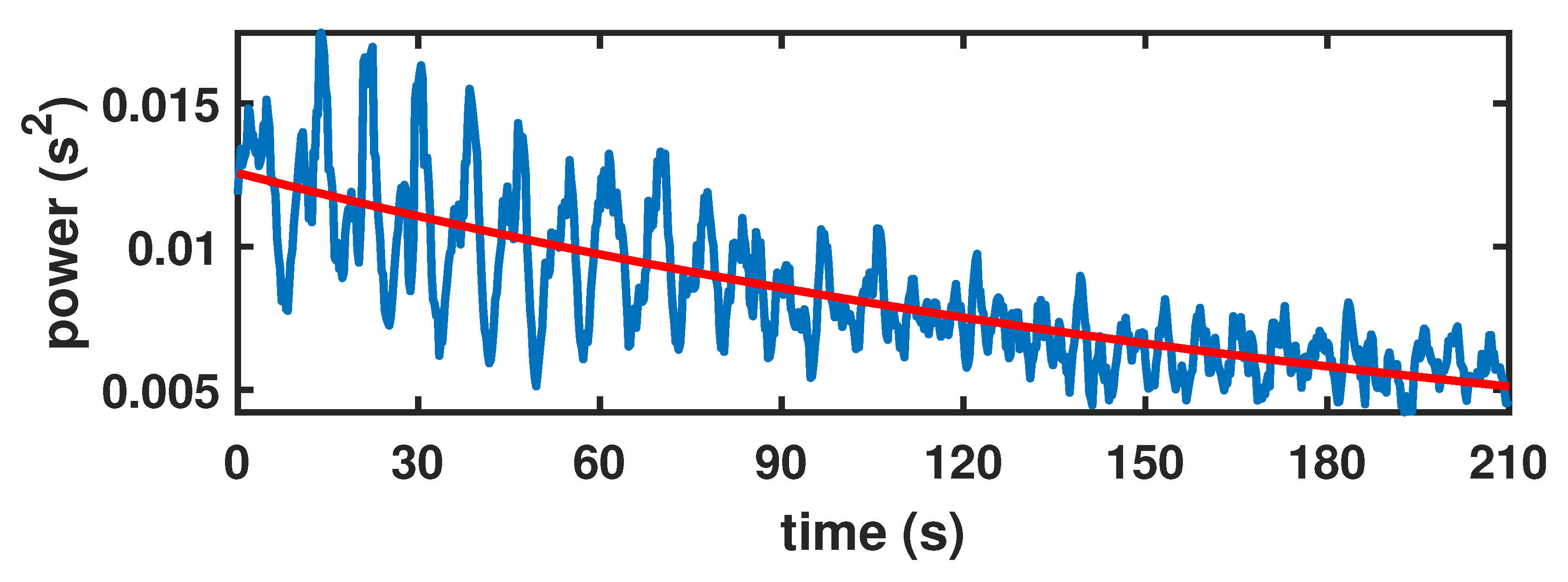
motivates the choice of the function q, see Figure 2. The value of the chirp parameters m , d and the parameters a , b , c must be estimated from the data.

2.3. Inference Method

Since a closed-form expression of the process distribution is not known, a maximum likelihood approach for estimating the model parameters is not feasible. In a previous contribution [23], we addressed the problem of fitting a real-valued LSP to sampled data by proposing the inference method HAnkel-Toeplitz Separation (HATS). The method hereby described is based on the same principle of dividing the inference problem into lower-dimensional sub-problems. The estimation procedure is summarized in Algorithm 1 and described in detail below.
Algorithm 1: Inference for LSCP parameters
Input:  Zero mean time-series data, both respiratory signal and corresponding HRV.
Output:  Estimated chirp parameters m ^ , d ^ and estimated LSP parameters a ^ , b ^ , c ^ .
Chirp estimation (
1  Estimate the instantaneous frequency of the chirp from the the respiratory signal, by taking the frequency of maximum power in the chirp range from a TF representation of the signal;
2  Find m ^ , d ^ and the corresponding covariance matrix F ^ I by fitting the linear chirp to the instantaneous frequency of the respiratory data;
LSP estimation
3  Compute the instantaneous power P ^ from the HRV data;
4  Find a ^ , b ^ by fitting the model function q to P ^ ;
5  Find c ^ by fitting R F ^ I to R ^ F = C ^ S C M Q ^ where R is the stationary covariance matrix of the model function r, C S C M is the estimated sample covariance matrix of the HRV data and Q ^ is the corresponding Hankel matrix based on the model q with parameters a ^ , b ^ ;
Return m ^ , d ^ , a ^ , b ^ , c ^ .
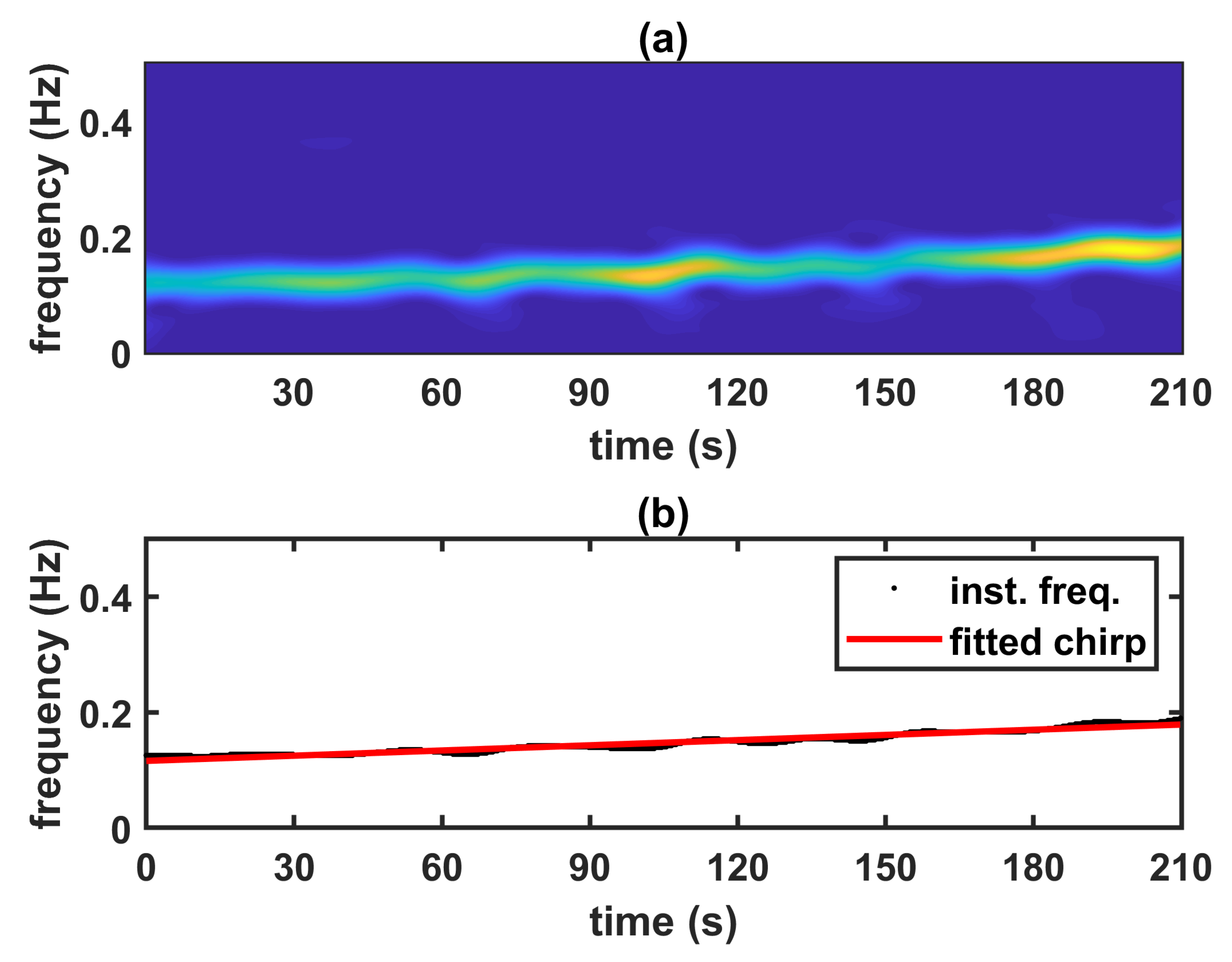
The first step is estimating the instantaneous frequency of the chirp from the respiratory signal, by taking the frequency of maximum power in the chirp range (frequencies above 0.12 Hz) of the spectrogram with Hanning window of 128 samples (32 s). The parameters m ^ and d ^ are estimated through a robust least square fitting of the linear chirp m t m d to the estimated instantaneous frequency of the respiratory signal. A corresponding chirp covariance matrix F ^ I is constructed according to the model Equation (2), where the covariance matrix values are F ^ I t 1 , t 2 = f I t 1 , t 2 . The estimation of the chirp from the respiratory signal of each TP allows accounting for the individual differences in the interpretation of the task of breathing accordingly to the metronome. An example of linear chirp fitted to the instantaneous frequency extracted from the spectrogram is presented in Figure 3.
At this point, a variation of the inference methods HATS can be used to compute the LSP parameters. First the function q in Equation (4) is fitted to the instantaneous power estimate P ^ ( t ) = x 2 ( t ) , where x ( t ) is the zero-mean adjusted HRV at time t, as in Equation (6), obtaining the estimated parameters a ^ and b ^ , from which the Hankel matrix Q ^ , with values Q ^ t 1 , t 2 = q ^ ( t 1 + t 2 ) / 2 , can be calculated.
The next step is computing the ordinary sample covariance matrix of the HRV data C ^ S C M . Thereafter, the Hadamard division of C ^ S C M by Q ^ provides the estimate R ^ F = C ^ S C M Q ^ , where R F corresponds to a non-stationary covariance matrix with values R F t 1 , t 2 = r t 1 t 2 · f I t 1 , t 2 . The parameter c ^ is obtained by fitting the model stationary covariance matrix R obtained from Equation (5), Hadamard multiplied with the chirp matrix F ^ I , to R ^ F .
Note that the division by the chirp matrix must be avoided for numerical issues as the chirp matrix F ^ contains values close to 0, differently from Q ^ , which is a strictly positive matrix.

2.4. Mean Square Error Optimal Time-Frequency Kernel

The MSE optimal model based TF smoothing kernel can be derived and evaluated once the model parameters of the LSCP are estimated. In the following, F f denotes the Fourier transform of the function f.
The Wigner-Ville spectrum (WVS) of an LSP is defined as
W ( t , ω ) = E X t + τ 2 X t τ 2 e i ω τ d τ = q ( t ) · F r ( ω )
[19,20], and the corresponding ambiguity spectrum as
A ( θ , τ ) = E X t + τ 2 X t τ 2 e i θ t d t = F q ( θ ) · r ( τ ) .
Any TF representation member of the Cohen’s class can be expressed as
W C ( t , ω ) = A ( θ , τ ) Φ ( θ , τ ) e i ( ω τ θ t ) d τ d θ ,
where Φ is an ambiguity kernel [11]. In [20], the MSE optimal kernel for circularly symmetric LSPs with Gaussian marginals has been derived as
Φ 0 ( θ , τ ) = | A ( θ , τ ) | 2 2 π ( | A ( θ , τ ) | 2 + B ( θ , τ ) ) ,
with
| A ( θ , τ ) | 2 = | F q ( θ ) | 2 | r ( τ ) | 2 , B ( θ , τ ) = ( F | r | 2 ( θ ) ) ( F 1 | F q | 2 ( τ ) ) .
The separable functions in Equation (11) are calculated according to the introduced model Equations (4) and (5) as
| r ( τ ) | 2 = e ( c / 4 ) τ 2 , F | r | 2 ( θ ) = 4 π c e ( θ 2 / c ) , F q ( θ ) = 0 + a e ( b i θ ) τ d τ = a b + i θ , | F q ( θ ) | 2 = a b + i θ 2 = a 2 b 2 + θ 2 , F 1 | F q | 2 ( τ ) = F 1 a 2 b 2 + θ 2 = a 2 2 b e b | τ | .
The modification of the LSP kernel for LSCP is based on the fact that if a signal g 0 ( t ) is multiplied as g ( t ) = g 0 ( t ) · e i · ( m 2 ) t 2 then the WVS is coordinate transformed as W ( t , ω ) W ( t , ω m · t ) . From [20], we accordingly find the optimal kernel to become
Φ ( θ , τ ) = Φ 0 ( θ m · τ , τ ) .
The multitaper approach allows efficient estimation as a weighted sum of windowed spectrograms
W C ( t , ω ) = E k = 1 K w k X ( s ) h k ( t s ) e i ω s d s 2 ,
with weights w k , and windows h k ( t ) , k = 1 K , given by the eigenvalues α and eigenvectors q respectively solution to
Ψ r o t ( s , t ) q ( s ) d s = α q ( t ) ,
where the Hermitian rotated time-lag kernel is defined as
Ψ r o t ( s , t ) = Ψ s + t 2 , s t ,
with
Ψ ( t , τ ) = Φ ( θ , τ ) e i t θ d θ
as in [20,21].

2.5. Regression Analysis

We performed a regression analysis [24] to search for the physiological factors that determine individual differences in the LSCP model parameters, exploring the predictive power of several physiological factors of interest: Gender (male, female), Age (years), Weight (kg), BMI (kg/m 2 ), State and Trait scores from the Spielberg State-Trait Anxiety Inventory (STAI) [25] and score in the Shirom-Melamed Burnout Questionnaire (SMBQ) [26,27,28]. Previous studies have validated the Swedish version of the STAI [29,30,31] and the SMBQ [32,33]. It is interesting considering both STAI and SMBQ measures since burnout consists of a combination of physical fatigue, emotional exhaustion, and cognitive weariness, not interchangeable with depression and anxiety [33,34].
The numerical variables were also modelled as categorical. We describe those that became relevant in the analysis. The categorical variable Age Groups divides the TPs in three categories of age: 20–30, 30–40, and over 40 years old. The categorical variable Stress, based on the value of SMBQ, divides the TPs into the following three groups: Low-Stressed ( SMBQ < 1 ); In-Between ( SMBQ [ 2.75 , 3.75 ) ); pre-stage Exhaustion Disorder (Pre-ED, SMBQ > 3.75 ). The variable Fit, based on BMI, has the following standard levels: Underweight ( BMI < 18.5 ); Normal ( BMI [ 18.5 , 25 ) ); Overweight ( BMI [ 25 , 30 ) ); Obese ( BMI > = 30 ).
Simple regression (i.e., regression models with a single explanatory variable) was tested first to isolate the effect of every factor, and then multivariate models were evaluated based on the statistical significance of the predictors (significance level of 0.1 ), the adjusted coefficient of determination R adj 2 , and the Akaike Information Criterion (AIC). Regression diagnostics included residual analysis, F-test for testing inclusion of variables, detection and treatment of outliers and influential observations.

3. Results and Discussion

3.1. Inference on the Model Parameters

The optimization steps in Algorithm 1 for estimating the parameters a , b , c were constrained so that a ( 0 , 5 ] , b ( 0 , 1 ] , c ( 0 , 10 ] . In Table 2, we report the mean, median, standard deviation and coefficient of variation c v of the individually estimated LSCP parameters for the 92 TPs ( LSCP i ). These values can be compared with the parameters estimated from a common LSCP ( LSCP c ) with 92 realizations, giving one set of parameters for all TPs. These parameter estimates are similar to the medians and means of the LSCP i parameters, with the exception of the parameter b related to the rate of the instantaneous power decrease during the chirp-breathing task, whose mean is almost 3 times larger than the median. The parameters with larger variations are those that determine the strongest individual differences among TPs.

3.2. Comparison between Time-Frequency Estimates

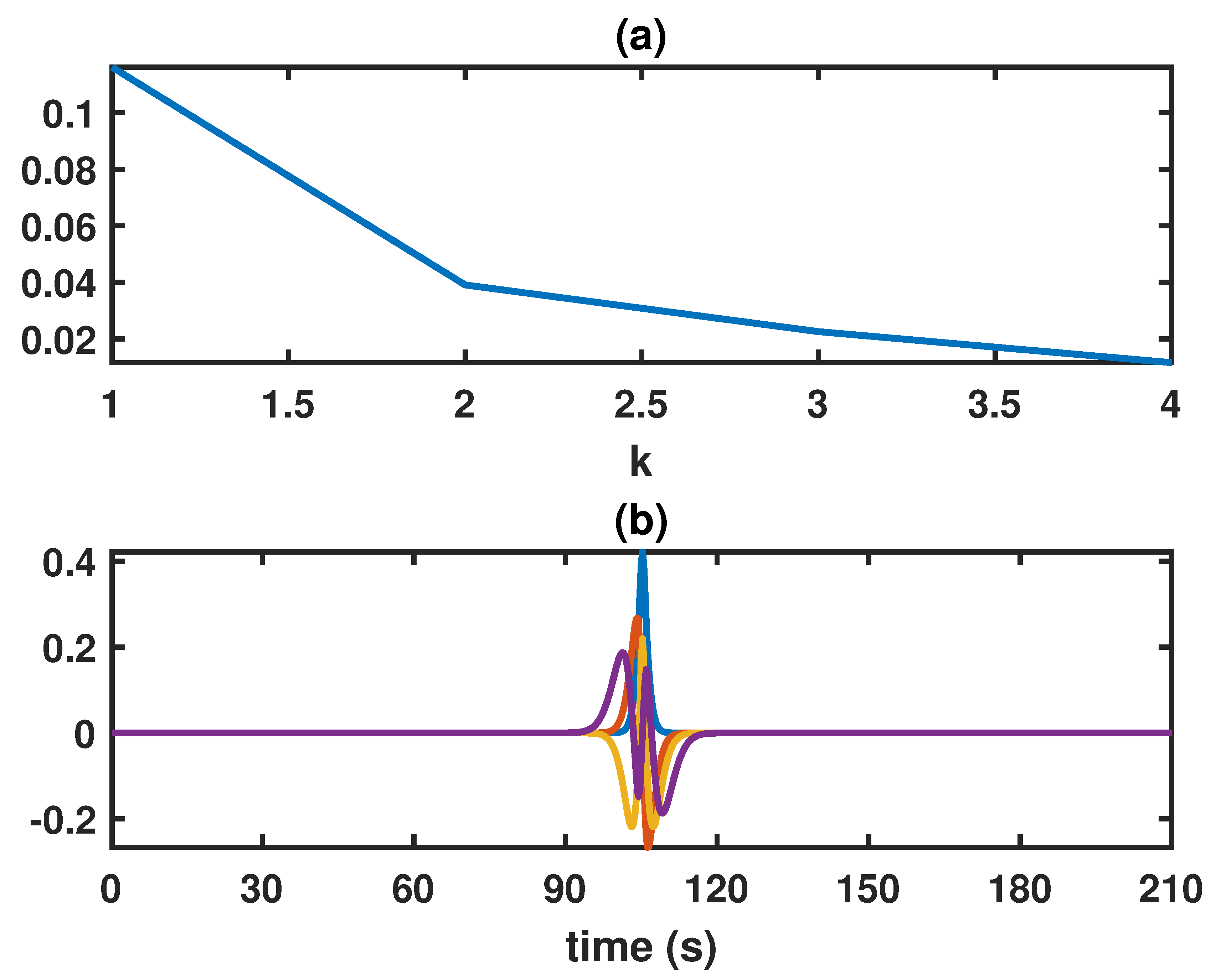
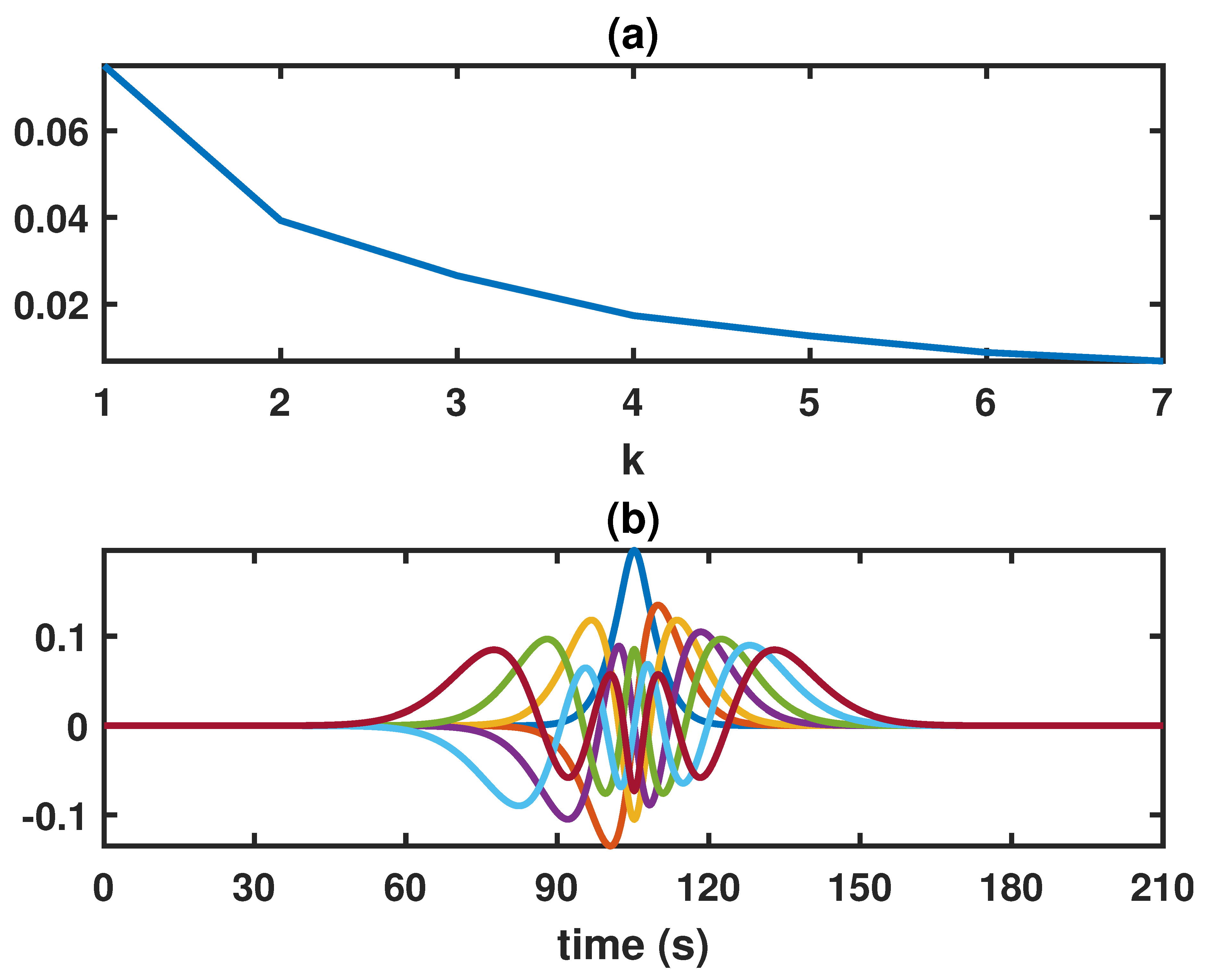
The MSE optimal eigenvectors and eigenvalues, corresponding to multitapers and weights of the MSE optimal LSCP c spectral estimator, are shown in Figure 4. These will in general differ from the MSE optimal eigenvectors and eigenvalues based on the individually estimated parameters, used for computing the MSE optimal LSCP i spectral estimator, an example of which can be seen in Figure 5. In particular, the number of eigenvalues significantly different from zero varies depending on the parameters.
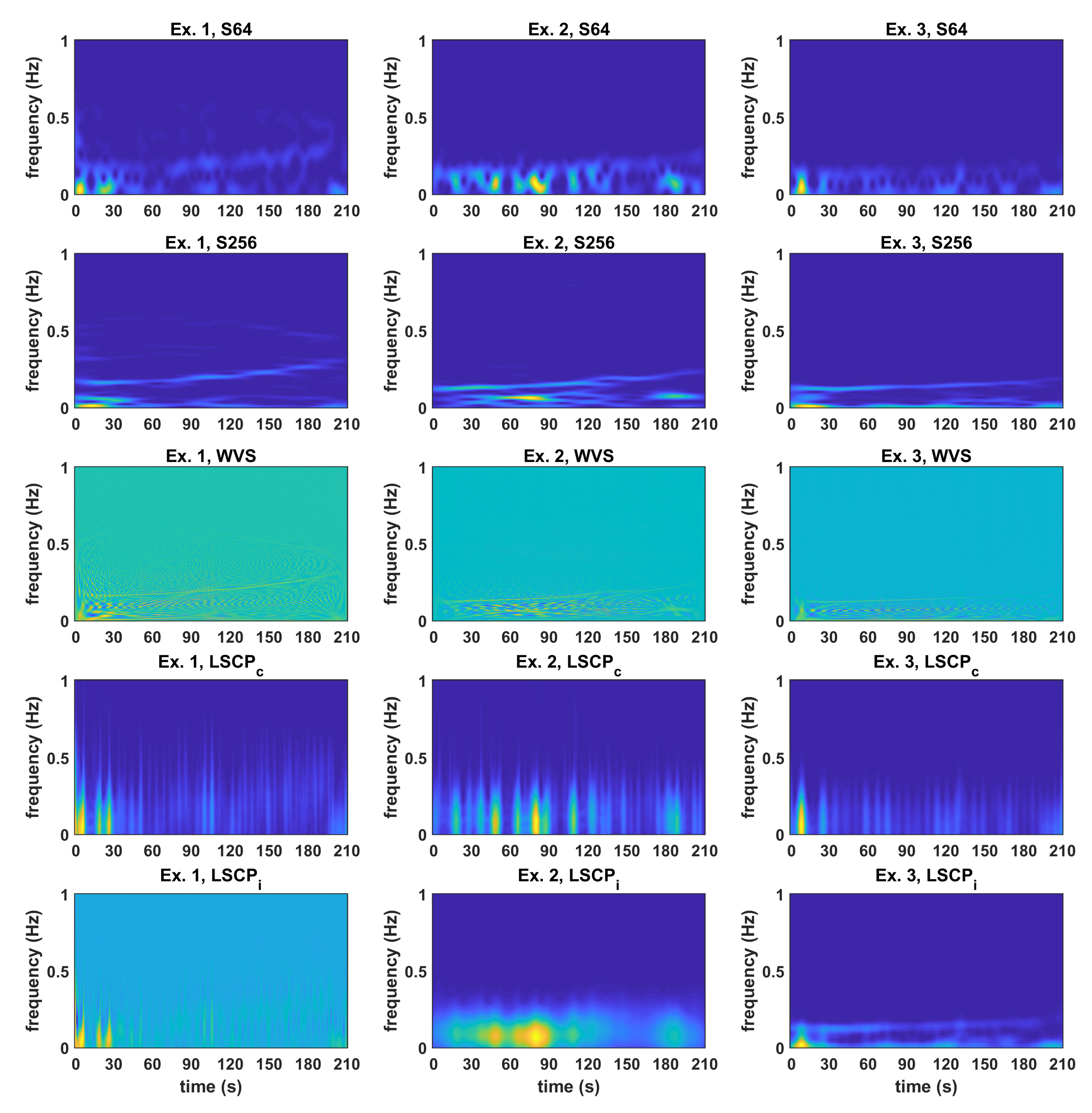
In Figure 6, we present examples of TF estimates for three TPs, obtained with the spectrogram with 64 samples Hanning window (16 s) S64, the spectrogram with 256 samples Hanning window (64 s) S256, the Wigner-Ville spectrum WVS, the MSE optimal LSCP c spectrum, and the MSE optimal LSCP i spectrum. The number of tapers K used for computing the LSCP i spectrum is dependent on the individual parameters. In the examples shown in Figure 6, K is equal to 10, 19, 3 for Ex. 1, Ex. 2, and Ex. 3 respectively.
The longer window spectrogram S256 offers a lower temporal resolution, compared to the shorter window spectrogram S64, while the opposite holds for the frequency resolution. Additionally to the resolution trade-off, the spectrogram suffers from a large variance, which is a significant problem when the estimate is based on a single realization of the underlying process, see the panels in the first two rows of Figure 6. The typical cross-terms of the WVS, large oscillating terms located in between the actual signal components, are visible in the panels in the middle row of Figure 6. By construction, the MSE optimal spectral estimators minimize bias and variance of the spectral estimates for LSCPs. LSCP i is preferred for capturing features that vary between the TPs, see panels in the last row of Figure 6. On the other hand, the LSCP c parameters are more robust than the individually estimated ones. This must be taken into account when the spectral estimates are used for extracting further features, e.g., frequency bands content from the time-frequency marginals or other spectral measures. It is worth noticing that for non-stationary signals of this kind, spectral measures such as the power in the low- and high- frequency bands and their ratio have limited interest, since the spectral content of the chirp signal is found above 0.12 Hz, which is above the usual low-frequency band.

3.3. Regression Analysis

In the following, we report and discuss the regression analysis results for the LSCP parameters.

3.3.1. Parameter m

The chirp parameters m and d determine the linear chirp describing the instantaneous frequency increase of the respiratory signal. These values differ among the TPs as a result of the individual interpretation of the chirp-breathing task.
The significant predictors of m in simple regression models are Age, State, Trait, and SMBQ. When considering multiple regression models including the predictor Age, only SMBQ is still significant, whereas the variables State and Trait cease to be significant. On the other hand, the variable Gender becomes significant in models including Age. The best multiple regression model according to both AIC and R adj 2 values includes Gender, Age, and SMBQ and achieves R adj 2 = 0.63 (Table 3). According to this model, an increase in age corresponds to an increase in the value of m. An opposite effect on m is given by being male respect to female and having a higher SMBQ.

3.3.2. Parameter d

The significant covariates in simple regression models for the parameter d are the same as for m, a fact that relates to the correlation between the two chirp parameters. None of the variables is still significant in multivariate models including the variable Age, therefore the selected model for d includes only the variable Age, with R adj 2 = 0.59 (Table 4).
For both m and d, even more explanatory than the numerical variable Age is the categorical variable Age Groups, that alone achieves R adj 2 = 0.79 and R adj 2 = 0.73 for m and d respectively. According to these models, being over the age 40 is what matters in affecting the value of the chirp parameters. However, only 10 TPs are older than 40 years, limiting the reliability of the last result.
To understand the meaning of the chirp parameters, a person older than 40 years would typically have the chirp parameter m approximately the double of the average values (i.e., m 0.0006 ) and the parameter d, representing the chirp delay, about half of the average value (i.e., d 200 ). These values correspond to an angular coefficient of the estimated linear chirp twice as large of the typical one, as a result of a steeper instantaneous frequency increase of the respiratory signal and consequently of the HRV.

3.3.3. Parameter a

The parameter a corresponds to the power at time zero, with a larger value of a corresponding to higher power, and it represents the amplitude multiplier that scales the exponential function. We consider the logarithmic transformation of a in the regression models to avoid positively skewed residuals.
Only the covariate Age is a significant predictor when considering models with a single explanatory variable. The regression model with only Age as predictor achieves R adj 2 = 0.24 . The same R adj 2 is obtained with the categorical variable Age, with all Age groups significantly different from the baseline. The strong correlation of the scaling parameter a with the variable Age is expected, since it is known that the HRV power decreases with age.
In multivariate models, both Age and Stress play a role, and the best predictive model includes them as categorical variables with R adj 2 = 0.27 (Table 5). According to this model, the value of log ( a ) is affected similarly by being in the age group 30–40 years old, compared to the baseline 20–30 years old, and having an SMBQ value compatible with pre-ED.
The fact that both Age and Stress are significant predictors of the value of log ( a ) with a similar effect (negative slope and same scale) suggests an analogy between the effect of aging and higher stress levels on the HRV instantaneous power. However, being in the age group over 40 years old has a 3.5 times stronger effect than having an SMBQ value compatible with pre-ED.

3.3.4. Parameter b

The value of b is related to the rate of the power decrease consequent to the increase in breathing frequency. The estimates of the parameter b show considerable large variability among the TPs, as indicated in Table 2. A higher value of b corresponds to a faster power decrease and does not point to a fault in the estimation; however, this large variability prevented the regression models from achieving high values of R adj 2 .
The only significant covariate in simple regression models is SMBQ. Step-wise model selection based on AIC led to a model including only SMBQ (Table 6), which however has a very low value of R adj 2 = 0.02 , reflecting the fact that much of the variability of the parameter b remains unexplained. After outliers and influential observations treatment, leading to the removal of 4 TPs, also the variables Gender, Age and Stress become significant in simple regression. The best multivariate model after removal of the 4 outliers has the covariates Gender, Age and Stress, with only the category pre-ED significantly different from the baseline (Table 7). This model has a higher R adj 2 = 0.11 .

3.3.5. Parameter c

The parameter c relates to the local stationarity of the underlying stochastic process, with smaller values of c indicating a long-lasting autocorrelation. Conversely, a larger value of the parameter c corresponds to a smaller standard deviation of the Gaussian bell in Equation (5), meaning faster decaying autocorrelation of the process.
In simple regression, all the variables Gender, Age, Weight, BMI, Fit, State, Trait, SMBQ and Stress are significant predictors of the parameter c. The step-wise selected multivariate model includes Gender, Age, and Fit, with only the category Obese significantly different from the baseline category Normal Weight (Table 8). This model has a coefficient of determination R adj 2 = 0.25 .
The most significant and clear predictor is Age, which has an effect of decreasing the value of c of 0.063 for each year of age. Fitness levels and being Male respect to Female have stronger effect than Age but they are not equally significant. It should be noted that Gender and BMI are correlated, with men having higher BMI than women, and recent studies suggest that the traditional BMI value might not be a good indicator of the fitness of a person.

4. Conclusions

In this paper, we propose a time-varying stochastic model, based on the definition of LSCPs, for task-related HRV measured during a novel chirp-breathing task. The proposed inference method allows the evaluation of the MSE TF spectrum, derived from the proposed stochastic model, using either individual model parameters or the parameters estimated from a common process. For comparison, other TF spectral estimates are computed, namely the spectrogram with different window lengths and the WVS without any smoothing kernel. The MSE optimal spectral estimator evaluated with the estimated parameters minimizes bias and variance of the spectral estimates for LSCPs, and therefore its use is preferable for extracting further features from the spectral estimates.
The LSCP model parameters are used as response variables in a regression analysis using several physiological covariates as predictors. The regression analysis shows correlation of the LSCP parameters with gender, age, levels of stress and fitness. The presented results are consistent with those of more extensive studies examining the relationship between HRV and physiological variables. Since each model parameter relates to a different aspect of the underlying LSCP, this approach may be useful to search for physiological factors that determine individual differences in the HRV.
The proposed complete framework for the study of task-related HRV in relation to factors describing both mental and physical health has general validity for the analysis of non-stationary data, and especially in the case of task-related HRV.
Further research can be addressed to identify new spectral measures to be extracted from the improved TF estimates since the traditional estimation of the spectral power divided in the low- and the high- frequency band is of limited interest for time-varying signals.

Author Contributions

Data curation, P.J.; Funding acquisition, M.S.; Investigation, R.A.; Methodology, R.A. and M.S.; Validation, R.A.; Writing—original draft, R.A.; Writing—review and editing, R.A. and M.S.

Funding

This research was funded by the eSSENCE strategic research programme.

Acknowledgments

A preliminary version of this work was presented as part of the Ph.D. thesis “Statistical inference and time-frequency estimation for non-stationary signal classification” by Rachele Anderson, defended at Centre for Mathematical Sciences, Lund University, Sweden, on the 4th of October 2019. The content here published has been used according to Lund University policy.

Conflicts of Interest

The authors declare no conflict of interest. The funders had no role in the design of the study; in the collection, analyses, or interpretation of data; in the writing of the manuscript, or in the decision to publish the results.

Abbreviations

The following abbreviations (in alphabetic order) are used in this manuscript:
AICAkaike information criterion
BMIbody-mass index
ECGelectrocardiography
HATSHankel-Toeplitz separation
HRVheart rate variability
LSCPlocally stationary chirp process
LSCP c LSCP with parameters estimated from a common process
LSCP i LSCP with individually estimated parameters
LSPlocally stationary process
MSEmean square error
R adj 2 adjusted coefficient of determination R square
RSArespiratory sinus arrhythmia
SMBQShirom-Melamed Burnout Questionnaire
STAISpielberg State-Trait Anxiety Inventory
S64spectrogram with 64 samples Hanning window
S256spectrogram with 256 samples Hanning window
TFtime-frequency
TPtest participant
WVSWigner-Ville spectrum

References

  1. Laborde, S.; Mosley, E.; Mertgen, A. A unifying conceptual framework of factors associated to cardiac vagal control. Heliyon 2018, 4, e01002. [Google Scholar] [CrossRef] [PubMed]
  2. Hernando, D.; Hernando, A.; Casajus, J.A.; Laguna, P.; Garatachea, N.; Bailón, R. Methodological framework for heart rate variability analysis during exercise: Application to running and cycling stress testing. Med. Biol. Eng. Comput. 2018, 56, 781–794. [Google Scholar] [CrossRef] [PubMed]
  3. Jönsson, P.; Österberg, K.; Wallergård, M.; Hansen, Å.M.; Garde, A.H.; Johansson, G.; Karlson, B. Exhaustion-related changes in cardiovascular and cortisol reactivity to acute psychosocial stress. Physiol. Behav. 2015, 151, 327–337. [Google Scholar] [CrossRef] [PubMed]
  4. Voss, A.; Schroeder, R.; Heitmann, A.; Peters, A.; Perz, S. Short-Term Heart Rate Variability - Influence of Gender and Age in Healthy Subjects. PLoS ONE 2015, 10, 1–33. [Google Scholar] [CrossRef]
  5. Gurel, N.Z.; Carek, A.M.; Inan, O.T.; Levantsevych, O.; Abdelhadi, N.; Hammadah, M.; O’Neal, W.T.; Kelli, H.; Wilmot, K.; Ward, L.; et al. Comparison of autonomic stress reactivity in young healthy versus aging subjects with heart disease. PLoS ONE 2019, 14, e0216278. [Google Scholar] [CrossRef]
  6. Woo, J.M.; Kim, T.S. Gender Plays Significant Role in Short-Term Heart Rate Variability. Appl. Psychophysiol. Biofeedback 2015, 40, 297–303. [Google Scholar] [CrossRef]
  7. Lennartsson, A.; Jonsdottir, I.; Sjörs, A. Low heart rate variability in patients with clinical burnout. Int. J. Psychophysiol. 2016, 110, 171–178. [Google Scholar] [CrossRef]
  8. Lindgren, G.; Rootzén, H.; Sandsten, M. Stationary Stochastic Processes for Scientists and Engineers; Chapman and Hall/CRC: Boca Raton, FL, USA, 2014. [Google Scholar]
  9. Valderas, M.T.; Bolea, J.; Laguna, P.; Bailón, R.; Vallverdú, M. Mutual information between heart rate variability and respiration for emotion characterization. Physiol. Meas. 2019, 40, 084001. [Google Scholar] [CrossRef]
  10. Liu, B.; Yan, S.; Wang, X.; Xie, L.; Tong, J.; Zhao, F.; Di, X.; Yan, X.; Zhang, J. An improved method to evaluate heart rate variability based on time-variant cardiorespiratory relation. J. Appl. Physiol. (Bethesda Md. 1985) 2019, 127, 320–327. [Google Scholar] [CrossRef]
  11. Cohen, L. Time-Frequency Analysis; Signal Processing Series; Prentice-Hall: Upper Saddle River, NJ, USA, 1995. [Google Scholar]
  12. Gates, K.M.; Gatzke-Kopp, L.M.; Sandsten, M.; Blandon, A.Y. Estimating time-varying RSA to examine psychophysiological linkage of marital dyads. Psychophysiology 2015, 52, 1059–1065. [Google Scholar] [CrossRef]
  13. Anderson, R.; Jönsson, P.; Sandsten, M. Insights on Spectral Measures for HRV Based on a Novel Approach for Data Acquisition. In Proceedings of the 2018 40th Annual International Conference of the IEEE Engineering in Medicine and Biology Society (EMBC), Honolulu, HI, USA, 17–21 July 2018; pp. 510–513. [Google Scholar] [CrossRef]
  14. Billman, G.E. Heart Rate Variability—A Historical Perspective. Front. Physiol. 2011, 2, 86. [Google Scholar] [CrossRef] [PubMed]
  15. Weippert, M.; Behrens, K.; Rieger, A.; Kumar, M.; Behrens, M. Effects of breathing patterns and light exercise on linear and nonlinear heart rate variability. Appl. Physiol. Nutr. Metab. 2015, 40, 762–768. [Google Scholar] [CrossRef]
  16. Hernando, A.; Lazaro, J.; Gil, E.; Arza, A.; Garzon, J.; Lopez-Anton, R.; De La Camara, C.; Laguna, P.; Aguilo, J.; Bailon, R. Inclusion of respiratory frequency information in heart rate variability analysis for stress assessment. IEEE J. Biomed. Health Inform. 2016, 20, 1016–1025. [Google Scholar] [CrossRef] [PubMed]
  17. Khan, N.A.; Jönsson, P.; Sandsten, M. Performance Comparison of Time-Frequency Distributions for Estimation of Instantaneous Frequency of Heart Rate Variability Signals. Appl. Sci. 2017, 7, 221. [Google Scholar] [CrossRef]
  18. Choi, J.; Gutierrez-Osuna, R. Removal of Respiratory Influences From Heart Rate Variability in Stress Monitoring. IEEE Sens. J. 2011, 11, 2649. [Google Scholar] [CrossRef]
  19. Silverman, R. Locally stationary random processes. IRE Trans. Inf. Theory 1957, 3, 182. [Google Scholar] [CrossRef]
  20. Wahlberg, P.; Hansson, M. Kernels and multiple windows for estimation of the Wigner-Ville spectrum of Gaussian locally stationary processes. IEEE Trans. Signal Process. 2007, 55, 73–84. [Google Scholar] [CrossRef]
  21. Hansson-Sandsten, M. Optimal Multitaper Wigner Spectrum Estimation of a Class of Locally Stationary Processes Using Hermite Functions. EURASIP J. Adv. Signal Process. 2011, 980805. [Google Scholar] [CrossRef]
  22. Anderson, R.; Jönsson, P.; Sandsten, M. Effects of Age, BMI, Anxiety and Stress on the Parameters of a Stochastic Model for Heart Rate Variability Including Respiratory Information. In Proceedings of the 11th International Joint Conference on Biomedical Engineering Systems and Technologies—Volume 3: BIOSIGNALS; SciTePress: Funchal, Madeira, Portugal, 2018; pp. 17–25. [Google Scholar] [CrossRef]
  23. Anderson, R.; Sandsten, M. Inference for time-varying signals using locally stationary processes. J. Comput. Appl. Math. 2019, 347, 24–35. [Google Scholar] [CrossRef]
  24. Rawlings, J.O.; Pantula, S.G.; Dickey, D.A. Applied Regression Analysis—A Research Tool, 2nd ed.; Springer: New York, NY, USA; London, UK, 1998. [Google Scholar]
  25. Spielberger, C.D.; Gorsuch, R.L. Manual for the State-Trait Anxiety Inventory, STAI (Form Y); Consulting Psychologists Press: Palo Alto, CA, USA, 1983. [Google Scholar]
  26. Shirom, A. Burnout in work organization. In International Review of Industrial and Organizational Psychology; Cooper, C.L., Robertson, I., Eds.; Wiley: New York, NY, USA, 1989; pp. 25–48. [Google Scholar]
  27. Melamed, S.; Kushnir, T.; Shirom, A. Burnout and risk factors for cardiovascular diseases. Behav. Med. 1992, 18, 53–60. [Google Scholar] [CrossRef]
  28. Melamed, S.; Shirom, A.; Toker, S.; Berliner, S.; Shapira, I. Burnout and Risk of Cardiovascular Disease: Evidence, Possible Causal Paths, and Promising Research Directions. Psychol. Bull. 2006, 132, 327–353. [Google Scholar] [CrossRef] [PubMed]
  29. Hansen, Å.M.; Hogh, A.; Persson, R.; Karlson, B.; Garde, A.H.; Ørbæk, P. Original article: Bullying at work, health outcomes, and physiological stress response. J. Psychosom. Res. 2006, 60, 63–72. [Google Scholar] [CrossRef] [PubMed]
  30. Persson, R.; Ørbæk, P. The influence of personality traits on neuropsychological test performance and self-reported health and social context in women. Personal. Individ. Differ. 2003, 34, 295–313. [Google Scholar] [CrossRef]
  31. Persson, R.; Österberg, K.; Karlson, B.; Ørbæk, P. The Meta-Contrast Technique: Relationships with personality traits and cognitive abilities in healthy women. Scand. J. Psychol. 2005, 46, 169–177. [Google Scholar] [CrossRef] [PubMed]
  32. Grossi, G.; Perski, A.; Evengård, B.; Blomkvist, V.; Orth-Gomér, K. Physiological correlates of burnout among women. J. Psychosom. Res. 2003, 55, 309–316. [Google Scholar] [CrossRef]
  33. Lundgren-Nilsson, Å.; Jonsdottir, I.H.; Pallant, J.; Ahlborg, G. Internal construct validity of the Shirom-Melamed Burnout Questionnaire (SMBQ). BMC Public Health 2012, 12. [Google Scholar] [CrossRef] [Green Version]
  34. Shirom, A. Job-related burnout: A review. In Handbook of Occupational Health Psychology; American Psychological Association: Washington, DC, USA, 2003; pp. 245–264. [Google Scholar]
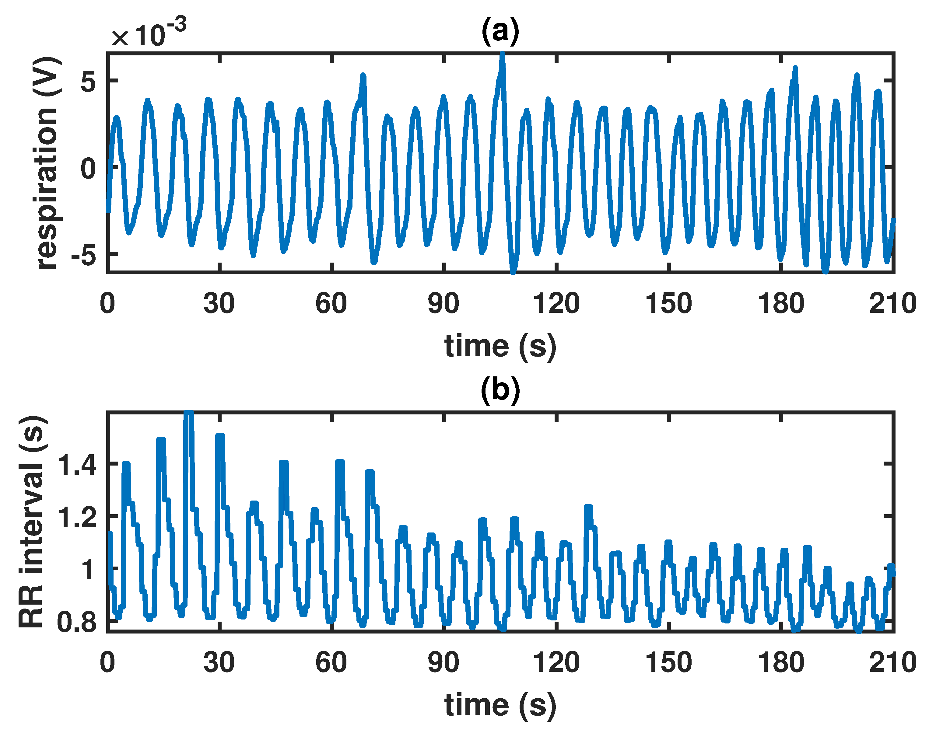
Figure 1. (a) Example of respiratory signal measured in Volt (V) and (b) HRV signal as tachogram, i.e., the sequence of the time intervals in seconds (s) between consecutive R-waves, of a subject recorded during the chirp-breathing task.
Applsci 09 05154 g001
Figure 2. Function q fitted to the mean instantaneous power of the 92 HRV time-series.
Applsci 09 05154 g002
Figure 3. (a) Spectrogram of a respiratory signal; (b) Red line is the linear chirp m t m d fitted to the instantaneous frequency (black dots) estimated from the spectrogram in (a).
Applsci 09 05154 g003
Figure 4. MSE optimal (a) eigenvalues and (b) eigenvectors, with K = 4 , corresponding to weights and multitapers of the MSE optimal LSCP c spectral estimator.
Applsci 09 05154 g004
Figure 5. An example of (a) eigenvalues and (b) eigenvectors, K = 7 , corresponding to weights and multitapers of the MSE optimal LSCP i spectral estimator, based on individual parameter estimates.
Applsci 09 05154 g005
Figure 6. Examples of the TF estimates obtained for three TPs with the spectral estimators considered: S64 (first row); S256 (second row); WVS (third row); the MSE optimal LSCP c spectrum (fourth row); the MSE optimal LSCP i spectrum (fifth row). All the spectra for one TP are in the same column.
Applsci 09 05154 g006
Table 1. Median, mean and standard deviation of the variables among the participants according to gender.
WomenMen
(n = 43)(n = 49)
MedianMeansdMedianMeansd
Age2528.057.862730.8410.42
Weight6263.569.707979.1410.39
BMI21.7721.972.7023.4524.233.05
State Anxiety3334.307.023031.737.76
Trait Anxiety3940.2510.333335.799.55
SMBQ3.053.401.202.592.951.16
Table 2. Median, mean, standard deviation and coefficient of variation c v of the estimated LSCP i parameters, and the estimated LSCP c parameters for the 92 TPs.
LSCP i LSCP c
ParameterMedianMeansd c v
m0.00030.00030.00010.31390.0003
d−396.36−379.1668.71−0.1812−402.62
a0.01110.01550.01621.04230.0126
b0.00520.01460.04623.17090.0043
c4.20233.90321.89510.48555.6208
Table 3. Regression model for parameter m.
Coeff. Est.S.E.p-Value
Gender (M) 2.826 × 10 5 1.322 × 10 5 0.0353
Age 8.156 × 10 6 7.310 × 10 7 < 2 × 10 16
SMBQ 1.175 × 10 5 5.760 × 10 6 0.0443
Table 4. Regression model for parameter d.
Coeff. Est.S.E.p-Value
Age5.67380.4896< 2 × 10 16
Table 5. Regression model for l o g ( a ) .
Coeff. Est.S.E.p-Value
Age 30–40−0.52220.22940.0253
Age > 40 −1.86620.3121 4.81 × 10 8
Stress (In-Between)−0.33410.22970.1494
Stress (Pre-ED)−0.49530.22840.0328
Table 6. Regression model for parameter b.
Coeff. Est.S.E.p-Value
SMBQ−0.0070820.0039940.07959
Table 7. Regression model for parameter b after removal of 4 outliers.
Coeff. Est.S.E.p-Value
Gender (M) 1.646 × 10 3 7.959 × 10 4 0.0417
Age 1.037 × 10 4 4.429 × 10 5 0.0215
Stress (Pre-ED) 1.898 × 10 3 8.653 × 10 4 0.0310
Table 8. Regression model for parameter c.
Coeff. Est.S.E.p-Value
Gender (M)−0.851400.365930.02233
Age−0.063540.018970.00121
Fit (Underweight)1.591920.970330.10453
Fit (Overweight)−0.125940.434460.77262
Fit (Obese)−2.438210.983780.01515