Artificial Intelligence-Based Controller for DC-DC Flyback Converter

Abstract

This paper presents an intelligent voltage controller designed on the basis of an adaptive neuro-fuzzy inference system (ANFIS) for a flyback converter (FC) working in continuous conduction mode (CCM). The union of fuzzy logic (FL) and adaptive neural networks (ANN) makes ANFIS more robust against model parameters’ uncertainties and perturbations in input voltage or load current. ANFIS inherits the advantages of structured knowledge representation from FL and learning capability from NN. Comparative analysis showed that the ANFIS controller offers not only the superior transient response characteristics, but also excellent steady-state characteristics compared to those of the FL controller (FLC) and proportional–integral–derivative (PID) controllers, thus validating its superiority over these traditional controllers. For this purpose, MATLAB/Simulink environment-based simulation results are presented for validation of the proposed converter compensated system under all operating conditions.

1. Introduction

DC-DC converters are employed in a variety of applications such as industrial controls, audio applications, power adapters and chargers, electric vehicles, electronic appliances, power supplies, renewable systems, aerospace equipment, and many other modern types of equipment that operate on DC [1,2,3]. Flyback converters (FCs) are a frequently used type of DC converter which may operate over a broad range of unregulated DC voltage. FCs serve as energy storage as well as converter isolation because of a choke in their topology. This results in reduced noise interference and provided load protection [4,5]. FCs are able to achieve high efficiency, high stability, small size, lightweight, less cost, etc., and have more power capacity (usually in the range of 20 to 200 W [6]) than other fundamental DC-DC converters. They are preferred for their outstanding features including output voltage waveform shape, power factor control optimization, and device miniaturization [7,8,9,10]. FCs exhibit non-minimum phase characteristics, i.e., the existence of a right half plane zero (RHPZ) in the voltage transfer function. This complicates the dynamics of FCs, as it results in increased gain and introduces additional phase lag, thus behaving as a pole. Thus, there is a need to design a feedback controller able to ensure the static and dynamic performance of the converter [11].

There are several analog and digital methods, such as PID, fuzzy logic (FL), and sliding mode control (SMC), for regulating the output of DC-DC FCs [12]. The feedback controller in a DC-DC converter is mainly responsible for delivering regulated supply, ideally with no steady-state error, less overshoot, and fast dynamic response while maintaining the highest possible efficiency [13,14]. Sliding mode control (SMC) based on the equivalent control method with a constant frequency has been applied to FCs in References [5,14]. In Reference [15], a peak current control technique for a flyback converter’s power factor correction was proposed. Reference [16] introduced average current mode control (ACM) for an FC, which employed an outer voltage feedback loop responsible for maintaining constant output voltage, and an inner loop engaged in sensing the input current. Quasi-resonant (QR) controllers for FCs have been presented in References [8,17,18]. PI controllers [19] and PID controllers [20,21] for FCs have also been reported in the literature. For example, in Reference [22], an FC with a photovoltaic (PV) panel was controlled by a PI compensator. The problem with these controllers is that they may not be robust against disturbance and uncertainty. Dynamic modeling and quantitative controller design of a current-mode controlled FC with optocoupler isolation were presented in Reference [23]. In Reference [24], the FC operated with a natural switching surface (NSS) control. Derivation and implementation of NSS with the operation of FCs in boundary conduction mode (BCM) were presented. A detailed review of the controllers to date, including pulse frequency modulation (PFM) control, adaptive peak current value control, current estimation control, and duty cycle control for FCs is presented in Reference [25].

Owing to features such as easier implementation and robustness characteristics, fuzzy logic controllers (FLCs) have also been employed to control FCs. FLCs are based on natural language and employ fuzzy “if-then” rules and fuzzy reasoning. They are tolerant of imprecise data, require fewer tuning parameters, and are flexible in such a way that they add more functionality without re-starting from the start [26,27]. Such an FLC can be employed to implement a central action for dealing with the variable structure nature of an FC. In Reference [28], an FLC-based FC is presented where the FLC responds rapidly to changes in load current or input voltage to ensure better load regulation. The controller also offers robustness with a good dynamic response. In Reference [29], a comparison was made between fuzzy and PI-based voltage controllers for an integrated buck flyback converter. Similarly, in Reference [30], the performance of the FC compensated system was analyzed via a PID controller and FLC. In these references, FLCs have outshone PIDs in terms of performance. Although an FL can make decisions based on the knowledge supplied to it, due to the lack of a training mechanism, it cannot make its knowledge adaptive.

More intelligence can be introduced to fuzzy rules by retuning them with artificial neural networks (ANN). ANFIS is the fusion of ANN and FL and utilizes the salient features of neural and fuzzy networks, respectively. The main advantage of ANFIS is that it converges quickly since it minimizes the search space dimensions of the backpropagation method used in NN [31,32,33]. An ANFIS-based maximum power point tracking (MPPT) system for a PV module with a DC-DC converter is presented in References [34,35,36,37]. In Reference [38], the authors proposed an ANFIS-based MPPT system comprising a PV module connected to a load through a DC-DC Ćuk converter to track the maximum power point (MPP). The MATLAB/Simulink environment was used to simulate the proposed model. Very limited research can be found in the literature regarding the control of switching converters using ANFIS. This paper thus proposes an ANFIS-based controller to regulate and improve the output voltage of FC. Line and load regulation and response to reference voltage changes are presented and the static and dynamic performance of the proposed controller is analyzed. Furthermore, its performance was also compared with FLC and PID controllers to validate its superiority.

The paper is organized as follows. Section 2 describes the modeling of an FC in continuous conduction mode (CCM). The design parameter selection of the FC used throughout the paper for the design of the controllers is described in Section 3. Section 4 presents the detailed controller design procedure for the FLC, ANFIS-based controller, and PID controller. Section 5 shows the results obtained after performing the simulations of FC with feedback controllers. Finally, the results are concluded in Section 6.

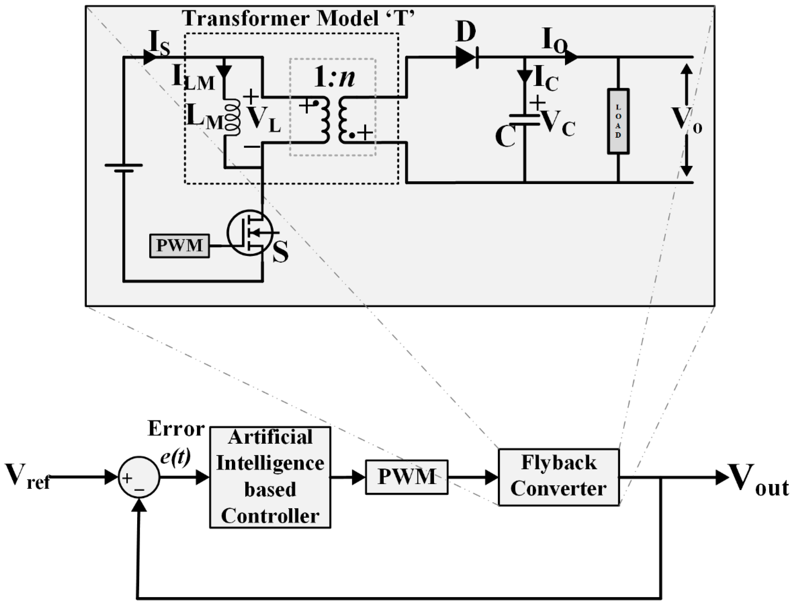
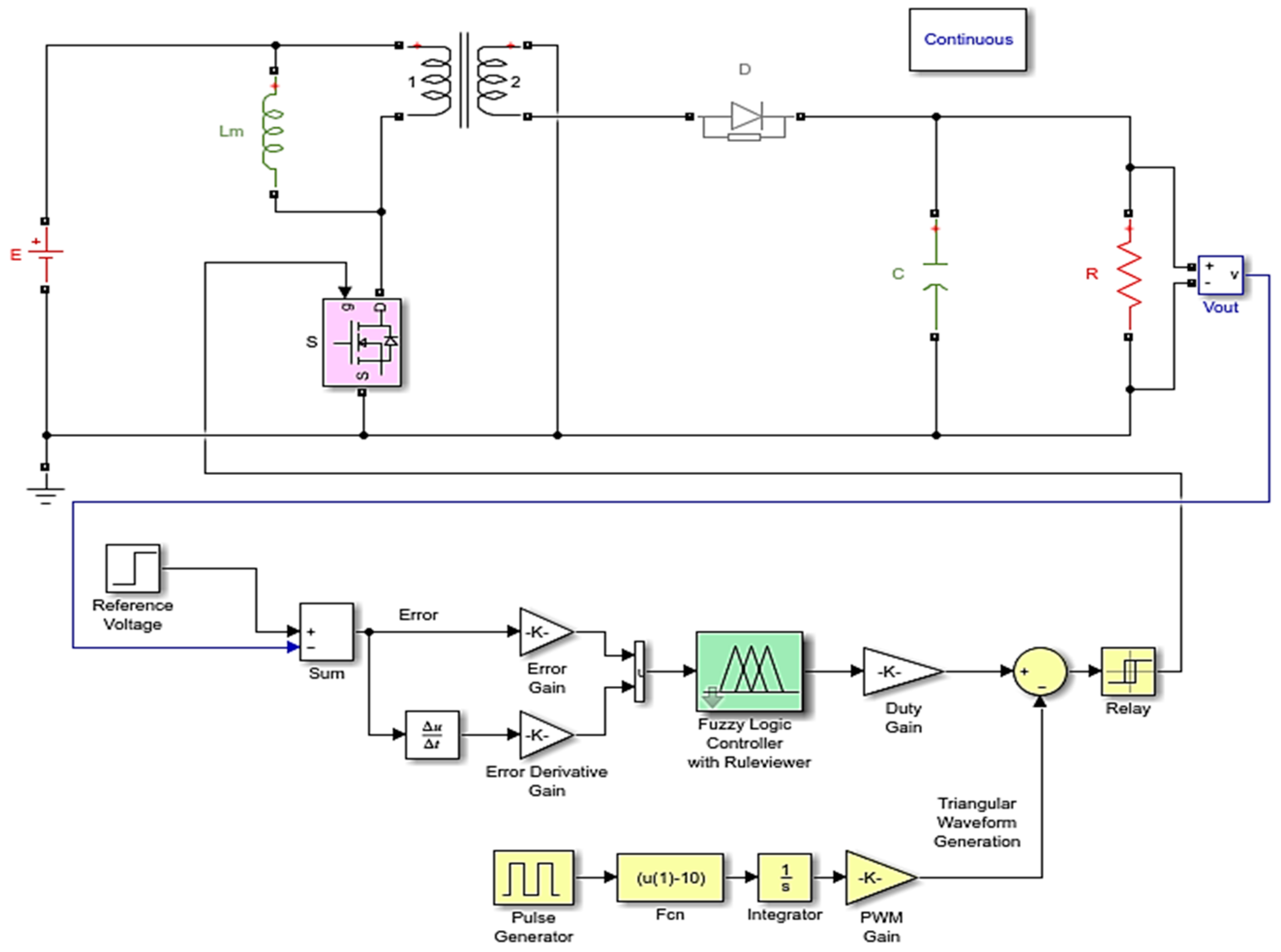
2. Modeling of Flyback Converter

The block diagram of the complete system, along with the circuit diagram of the FC, is presented in Figure 1. FC behaves like a plant to be controlled. To develop a controller for it, its dynamics must be known.

Figure 1 shows the FC circuit consisting of a DC voltage source “E”, a power MOSFET “S”, transformer “T” for isolation purposes, diode “D”, capacitor “C”, and load and magnetizing inductance of transformer “L_M”. The DC voltage source can be the output of an uncontrolled rectifier (after filtering) that converts AC to DC. The switching MOSFET S is fed with a PWM at high frequency. The purpose of the transformer is also to provide better matching between input and output voltage and current requirements. The diode D rectifies the secondary voltage of the transformer T. The capacitor C is for filtration purposes.

For determining FC dynamics in CCM, a state-space averaging technique was employed [5,24,28]. Inductor current $I_{LM}$ and voltage across the capacitor $V_C$ were considered as independent state variables of the state vector $X$. Thus,

$$X=\left[\begin{array}{c}{I}_{LM}\\ V_C\end{array}\right]$$

(1)

The independent input vector $u$ is expressed in Equation (2) with input voltage $E$ and voltage across the diode $V_D$ as constraints.

$$u=\left[\begin{array}{c}E\\ V_D\end{array}\right]$$

(2)

The output vector consists of input current $I_S$ and output voltage $V_O$, since in the modeling procedure, input and output are to be modeled, which are dependent quantities.

$$Y=\left[\begin{array}{c}{I}_S\\ V_O\end{array}\right]$$

(3)

CCM operation occurs in two modes:

Mode 1: When the switching MOSFET S is in ON state, current flows through the primary side of the transformer with magnitude $I_S$, and the diode is reversed biased at the secondary side. Therefore, no current flows in the secondary of the transformer. The capacitor’s stored energy supplies the output voltage. The state conditions for Mode 1 are:

$$\frac{d{I}_{LM}}{dt}=\frac{E}{L_M}-\frac{I_S{R}_S}{L_M}$$

(4)

$$\frac{d{V}_C}{dt}=-\frac{V_C}{(R+R_C)C}$$

(5)

$$V_O=\frac{V_{C}R}{R+R_C}$$

(6)

$$I_S=I_{LM}$$

(7)

where $L_M$ is the magnetizing inductance of transformer, $\frac{d{I}_{LM}}{dt}$ is the rate of change of current in the primary of the transformer, $E$ is the supply voltage, $I_S$ is the supply current, $R_S$ is the resistance of the switch S, $C$ is the capacitance, $\frac{d{V}_C}{dt}$ is the rate of change of capacitor voltage, $V_C$ is the capacitor voltage, $R$ is the load resistance, $R_C$ is the internal resistance of capacitor, and $V_O$ is the output voltage. Thus, the state-space representation for Mode 1 is as follows:

$$\dot{x}=Ax+Bu\Rightarrow \left[\begin{array}{c}\frac{d{I}_{LM}}{dt}\\ \frac{d{V}_C}{dt}\end{array}\right]=\left[\begin{array}{cc}-\frac{R_S}{L_M}& 0\\ 0& -\frac{1}{C\left(R+R_C\right)}\end{array}\right]\left[\begin{array}{c}{I}_{LM}\\ V_C\end{array}\right]+\left[\begin{array}{cc}\frac{1}{L_M}& 0\\ 0& 0\end{array}\right]\left[\begin{array}{c}E\\ V_D\end{array}\right]$$

(8)

$$y=Cx+Du\Rightarrow \left[\begin{array}{c}{I}_S\\ V_O\end{array}\right]=\left[\begin{array}{cc}1& 0\\ 0& -\frac{R}{R+R_C}\end{array}\right]\left[\begin{array}{c}{I}_{LM}\\ V_C\end{array}\right]+\left[\begin{array}{cc}0& 0\\ 0& 0\end{array}\right]\left[\begin{array}{c}E\\ V_D\end{array}\right]$$

(9)

where $x$ is a state vector, $\dot{x}$ is the state vector derivative with regard to time, $A$ is the system matrix, $B$ is the input matrix, $u$ is the input or control vector, $y$ is the output vector, $C$ is the output matrix, and $D$ is the disturbance matrix.

Mode 2: When the switching MOSFET S is in OFF state, current flows through the secondary of the transformer and the diode is forward biased. The energy stored in the magnetizing inductance $L_M$ is transferred to the load and output capacitor.

The state conditions for Mode 2 are:

$$\frac{d{I}_{LM}}{dt}=-\frac{n^2{I}_{LM}R{R}_C}{L_M(R+R_C)}-\frac{nR{V}_C}{L_M(R+R_C)}-\frac{n{V}_D}{L_M}$$

(10)

$$\frac{d{V}_C}{dt}=\frac{n{I}_{LM}R}{C(R+R_C)}-\frac{V_C}{C(R+R_C)}$$

(11)

$$V_O=\frac{nR{R}_C}{R+R_C}{I}_{LM}+\frac{R}{R+R_C}{V}_C$$

(12)

$$I_S=0$$

(13)

where $n$ is the turn ratio of the transformer. Thus, the state-space representation for Mode 2 is as follows:

$$\left[\begin{array}{c}\frac{d{I}_{LM}}{dt}\\ \frac{d{V}_C}{dt}\end{array}\right]=\left[\begin{array}{cc}-\frac{n^{2}R{R}_C}{L_M(R+R_C)}& -\frac{nR}{L_M(R+R_C)}\\ \frac{nR}{C\left(R+R_C\right)}& -\frac{1}{C\left(R+R_C\right)}\end{array}\right]\left[\begin{array}{c}{I}_{LM}\\ V_C\end{array}\right]+\left[\begin{array}{cc}0& -\frac{n}{L_M}\\ 0& 0\end{array}\right]\left[\begin{array}{c}E\\ V_D\end{array}\right]$$

(14)

$$\left[\begin{array}{c}{I}_S\\ V_O\end{array}\right]=\left[\begin{array}{cc}0& 0\\ \frac{nR{R}_C}{R+R_C}& \frac{R}{R+R_C}\end{array}\right]\left[\begin{array}{c}{I}_{LM}\\ V_C\end{array}\right]+\left[\begin{array}{cc}0& 0\\ 0& 0\end{array}\right]\left[\begin{array}{c}E\\ V_D\end{array}\right]$$

(15)

Now, the state-space averaged model for CCM can be written as [5]:

$$\begin{array}{l}\left[\begin{array}{c}\frac{d{I}_{LM}}{dt}\\ \frac{d{V}_C}{dt}\end{array}\right]=\left[\begin{array}{cc}-\frac{R_S}{L_M}{S}_1-\frac{n^{2}R{R}_C}{L_M(R+R_C)}{S}_2& -\frac{nR}{L_M(R+R_C)}{S}_2\\ \frac{nR}{C(R+R_C)}{S}_2& -\frac{1}{C(R+R_C)}\end{array}\right]\left[\begin{array}{c}{I}_{LM}\\ V_C\end{array}\right]\\ +\left[\begin{array}{cc}-\frac{1}{L_M}{S}_1& -\frac{n}{L_M}{S}_2\\ 0& 0\end{array}\right]\left[\begin{array}{c}E\\ V_D\end{array}\right]\end{array}$$

(16)

$$\left[\begin{array}{c}{I}_S\\ V_O\end{array}\right]=\left[\begin{array}{cc}0& 0\\ \frac{nR{R}_C}{R+R_C}{S}_2& \frac{R}{R+R_C}\end{array}\right]\left[\begin{array}{c}{I}_{LM}\\ V_C\end{array}\right]$$

(17)

Leading towards the derivation of the transfer function, the small-signal model was employed to approximate the behavior of the FC model. In the state-space model (SSM), state variables and control input are comprised of DC and AC quantities. Capital subscripts represent DC steady-state values, and small subscripts represent AC perturbations.

$$i_{LM}=I_{LM}+i_{lm}$$

(18)

$$v_O=V_O+v_o$$

(19)

$$D=\Delta +d$$

(20)

Inserting the above quantities into the state-space averaged model (SSAM) and hence taking Laplace transforms results in the voltage transfer function expressed in Equation (21).

$$H_{v_o}(s)=\frac{v_o}{d}=\frac{\left(-\frac{E{L}_M\Delta }{n{(1-\Delta )}^2}s+ER\right)}{\left(L_{M}RC\right)s^2+\left(L_M\right)s+\left(R{n}^2{(1-\Delta )}^2\right)}$$

(21)

The negative sign in the numerator with the term ‘s’ indicates that it is a non-minimum phase system, i.e., it has a right half plane zero (RHPZ).

3. Design of FC with Specifications

Let us consider the efficiency of FC to be 90%.

$$E_{LM}=\frac{1}{2}{L}_M{\left(I_{L{M}_{\max }}-I_{L{M}_{\min }}\right)}^2$$

(22)

$$P_{out}=\frac{1}{2}{L}_M{\left(I_{L{M}_{\max }}-I_{L{M}_{\min }}\right)}^2\times f_S\times \eta$$

(23)

For a 90% efficiency, $\eta$ = 0.9.

$$\eta =\frac{P_{out}}{P_{in}}\mathrm{and}{P}_{in}=\frac{P_{out}}{0.9}=1.11P_{out}$$

(24)

$$P_{out}=\frac{V_O{}^2}{R}$$

(25)

Substituting Equation (25) into Equation (24) gives Equation (26).

$$P_{in}=1.11\times \frac{V_O{}^2}{R}=\frac{\frac{1}{2}{L}_M{\left(I_{L{M}_{\max }}-I_{L{M}_{\min }}\right)}^2}{T_S}$$

(26)

where $\eta$ is the practical efficiency of the design, $I_{L{M}_{\max }}$ and $I_{L{M}_{\min }}$ are the maximum and minimum magnitudes of current $I_{LM}$, respectively, and $T_S$ is the reciprocal of $f_S$. For calculating the inductance and capacitance, the following formulae can be used:

$$L_M=\frac{V_S\times D}{2\pi \times f_S\times \Delta I}$$

(27)

$$C=\frac{V_S\times D^2}{n\left(1-D\right)R\times f_S\times \Delta V}$$

(28)

The typical parameter values used throughout the paper are tabulated in

Table 1. Designed values of flyback controller (FC) components.

Parameter/Component	Value
Input voltage $E$	12 V
Output voltage $V_O$	24 V
Transformer power	120 W
Magnetizing inductance of transformer $L_M$	250 μH
Output filter capacitor $C$	200 μF
Load resistance $R$	10 Ω
Duty cycle $D$	0.5
Transformer turn ratio $n_1/n_2=N$	0.5
Switching frequency $f_S$	100 kHz

.

With the above-mentioned design specifications, the FC with unity feedback showed output voltage across the resistive load with a peak value of 30.76 V and a steady-state voltage of 22.19 V, as shown in Figure 2. An intelligent controller needed to be introduced into the loop.

4. Controller Design

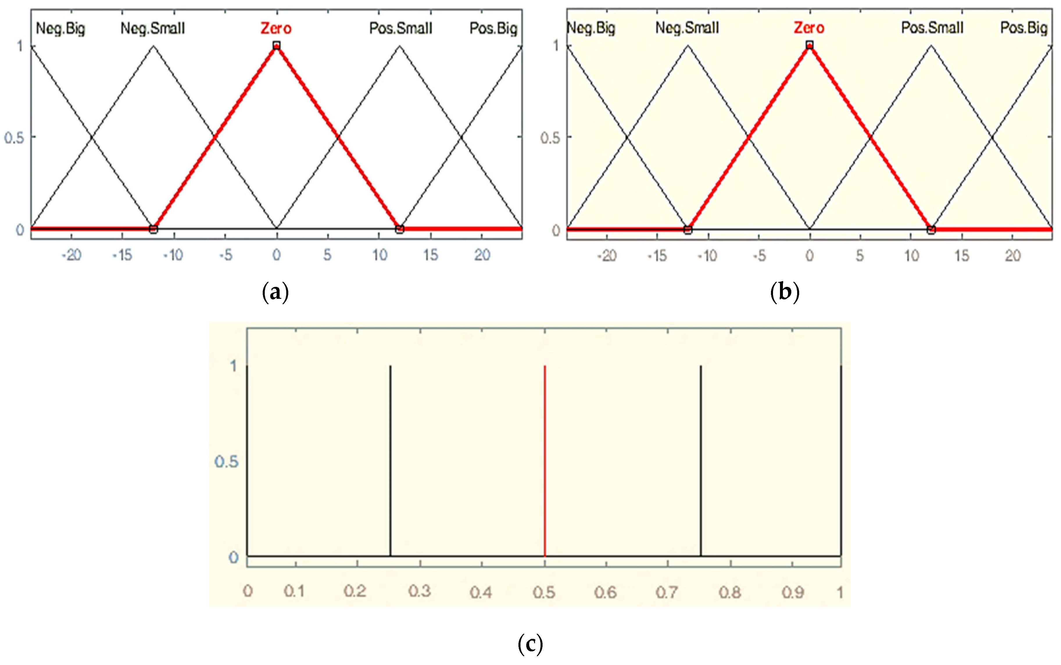
After describing the flyback converter modeling, a detailed design procedure of feedback controllers, i.e., FLC, ANFIS-based controller, and PID controller, is presented in this section.

4.1. FLC

Fuzzy logic (FL) is an extension of multivalued logic. It is related to the theory of fuzzy sets, which refers to classes of objects with blunt boundaries in which membership is a matter of degree. It emulates, unlike crisp data, the ability to reason and uses approximate data for finding solutions. FLCs are knowledge-based controllers that consist of linguistic if-then rules, which can be constructed by using the knowledge of experts in a particular field of interest. FLCs have shown their ability in many applications, especially in complex nonlinear systems, for which analytical modeling is difficult [39,40]. Figure 3 illustrates the block diagram of a traditional FLC system, which consists of four components: fuzzification interface (FI), rule-base (RB), inference mechanism (IM), and defuzzification interface (DI). The FI classifies the inputs into suitable linguistic values/sets. The RB is comprised of fuzzy sets (database) and fuzzy control rules. The IM is the kernel of the FLC, which is capable of simulating human decision making based on fuzzy concepts and inferring fuzzy control actions using fuzzy relations and rules of inference. The DI makes conclusions from the IM and gives an output, i.e., input for the plant [41,42].

Figure 4 presents the model of an FC with a fuzzy logic controller in MATLAB/Simulink. The output voltage is measured and is compared with the reference value, and thus, an error is generated. Two quantities, namely error e and derivative of the error Δe, are generated as the inputs for the fuzzy logic controller. The fuzzy logic controller processes the quantities based on membership functions (MFs) and fuzzy rules to generate an output, which is the duty cycle d. This signal is compared with a 100 kHz triangular waveform to generate duty cycle pulses for the gate of MOSFET S.

Input MFs are presented in Figure 5a,b. Five MFs were assigned to each input variable for the universe of discourse of −24 to 24. The output MFs of a Sugeno type FIS are constants or linear functions. In this case, constants were selected. Finite values were assigned to each MF, as shown in Figure 5c. FLC works based on fuzzy rules.

Table 2. Rules for the FLC.

	e	Neg. Big	Neg. Small	Zero	Pos. Small	Pos. Big
Δe
Neg. Big		0	0	0	0.25	0.5
Neg. Small		0	0	0.25	0.5	0.75
Zero		0	0.25	0.5	0.75	1
Pos. Small		0.75	0.5	0.75	1	1
Pos. Big		0.5	0.75	1	1	1

illustrates the fuzzy rules.

The 3D graphical representation of the rule surface relating output value for any combination of the two inputs is presented in Figure 6.

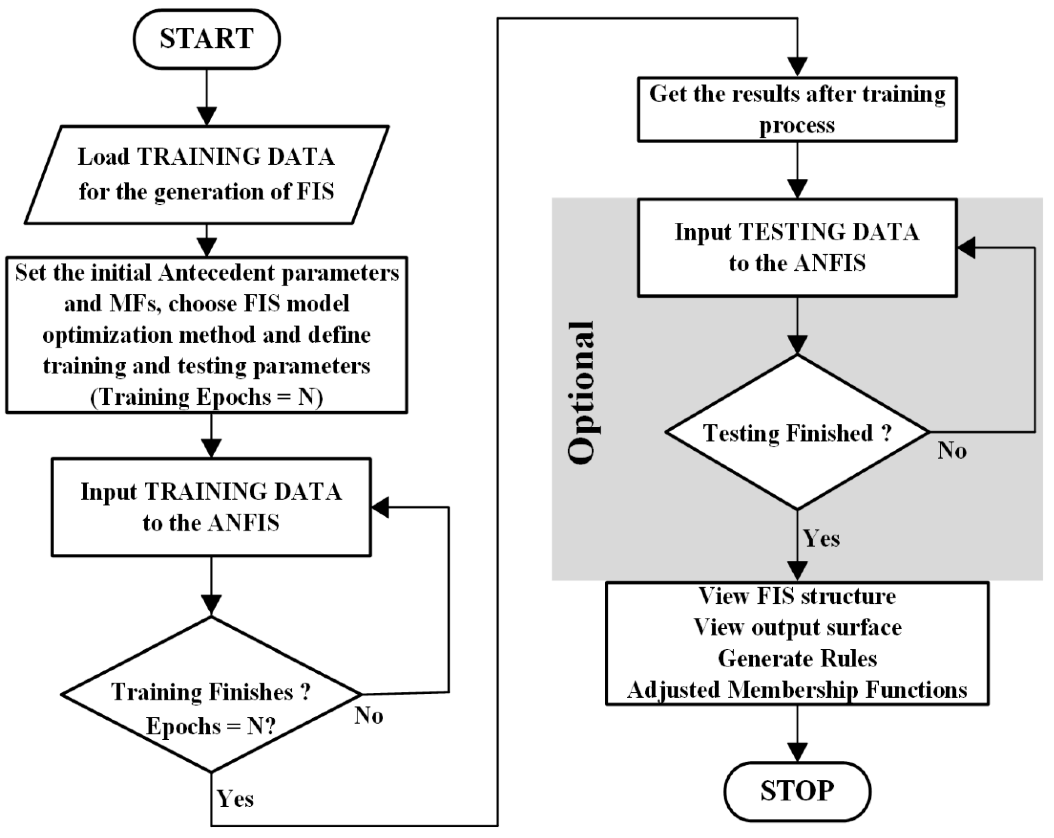
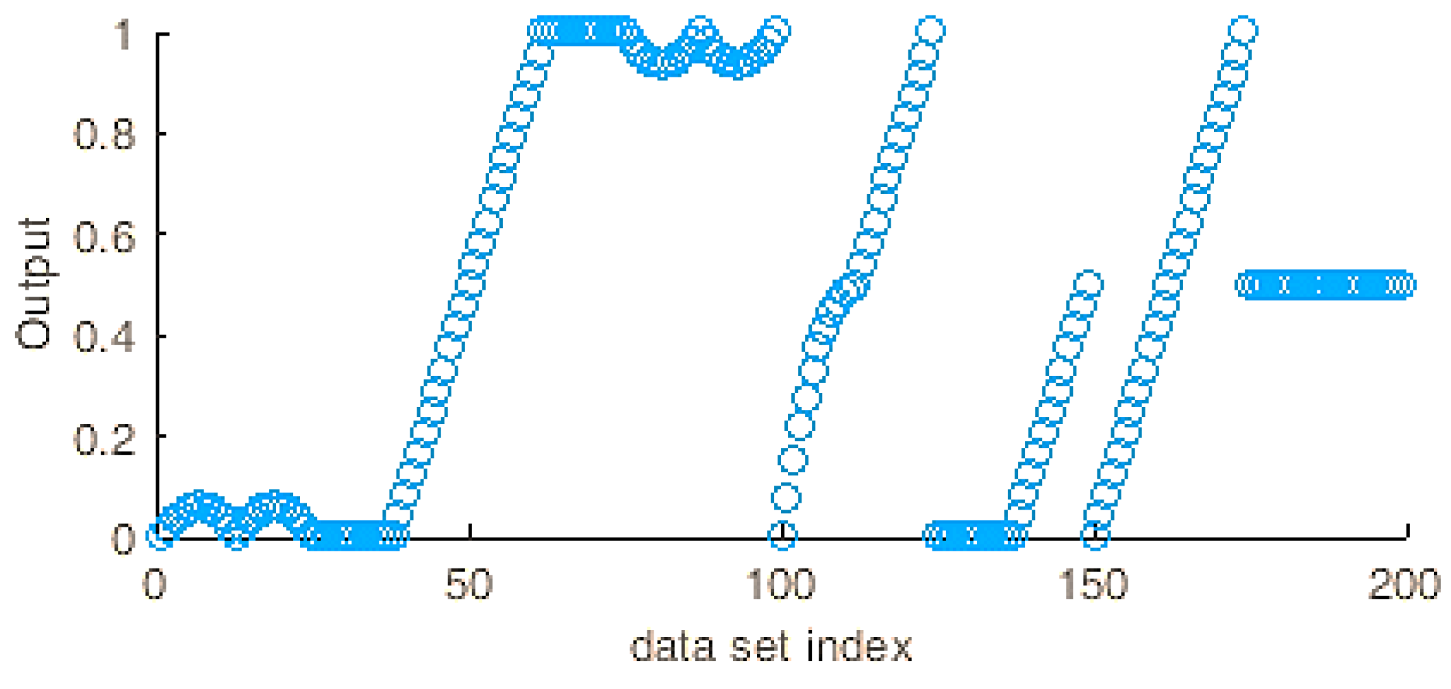
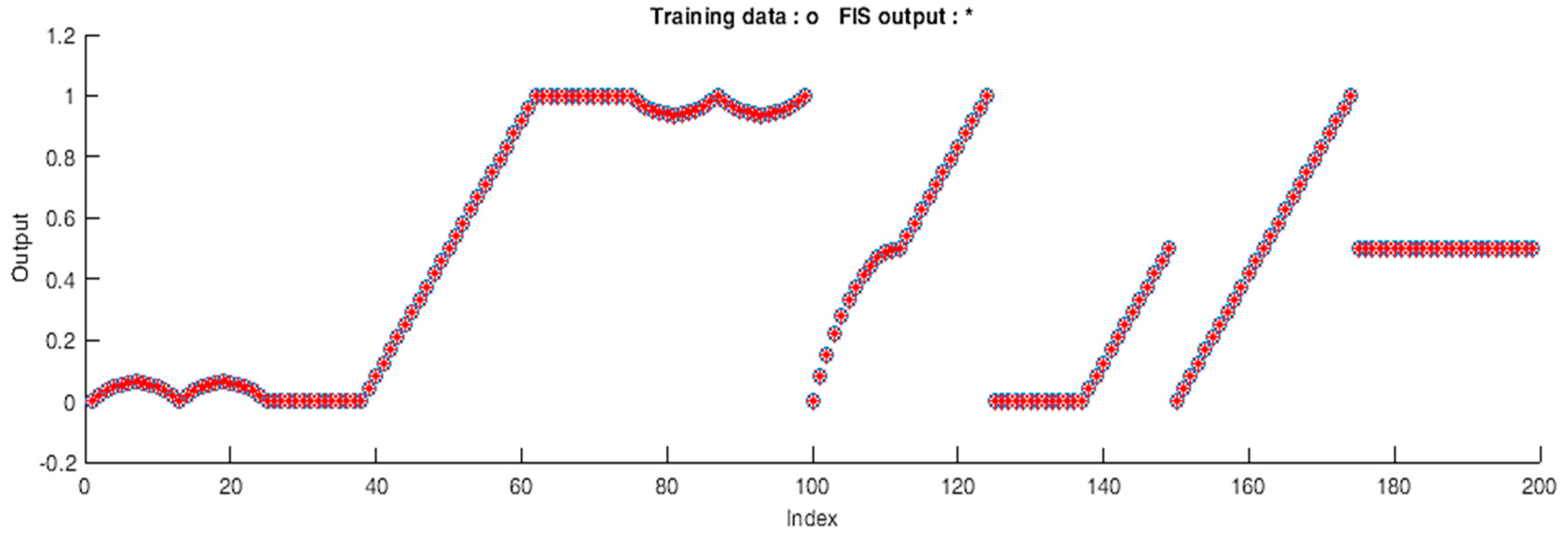
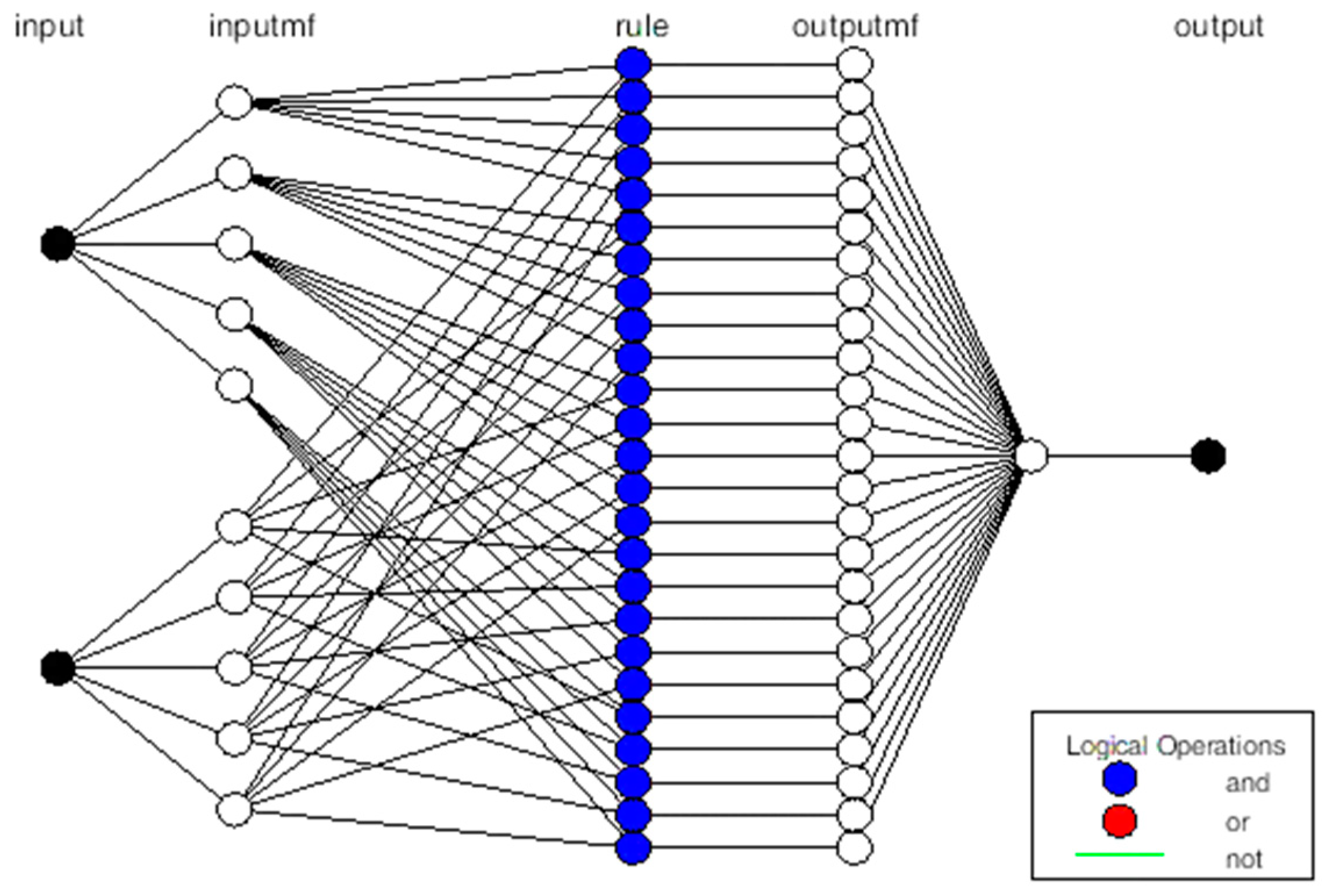
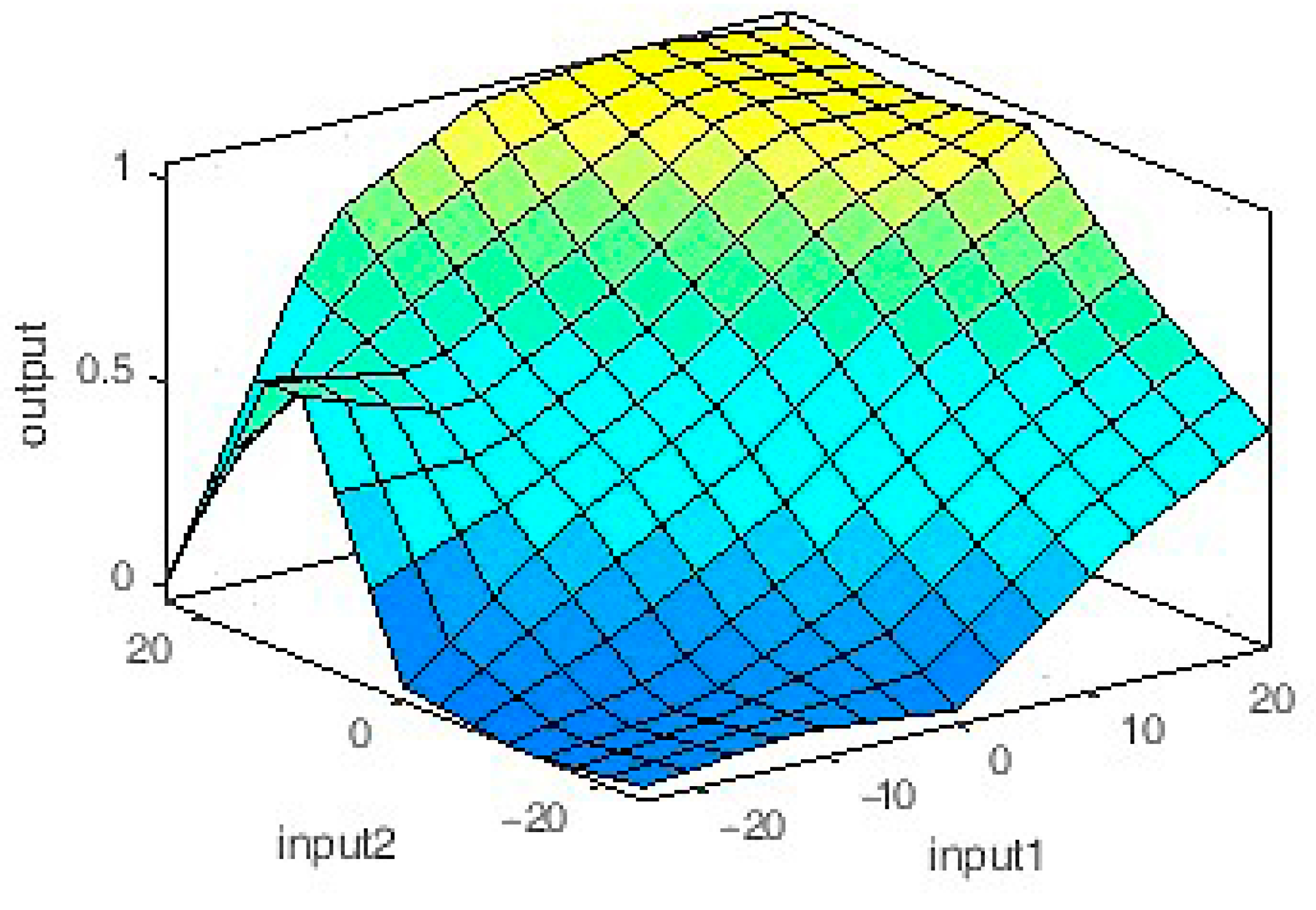
4.2. ANFIS-Based Controller

The adaptive neuro-fuzzy inference system (ANFIS) is the combination of fuzzy logic (FL) and neural networks (NN) developed by Jang in 1993 [43,44]. From FL and NN, it inherits their advantages, structured knowledge representation, and learning capabilities, respectively. In FL, membership functions and their distribution and fuzzy rules are obtained based on expert knowledge. In ANFIS, MFs and rules obtained from the FLC are further tuned using neural networks to generate optimized MFs, and thus rules [36,44,45].

ANFIS uses NN to adjust the parameters of MFs while tuning fuzzy rules. The ANN part of the ANFIS contributes to the reduction of error, thus optimizing the parameters. On the other hand, the FI part of the ANFIS deals with uncertainty efficiently. The purpose of ANFIS is to apply a hybrid learning algorithm, adopting input-output data sets and then accomplishment with a desired input-output mapping, to identify the optimal MFs and other parameters of the equivalent FIS [44,45,46].

ANFIS possesses a layered architecture similar to NN. Nodes in the layers can be adaptive or fixed. Adaptive and fixed nodes are illustrated by squares and circles in the architecture diagram, respectively. The general architecture of ANFIS (with five layers, as we considered in our work) is illustrated in Figure 7 [43,44,47,48].

The first order Sugeno type with two inputs “x”, i.e., e and “y”, i.e., Δe, and the rules for a Sugeno based ANFIS are expressed by Equations (29) and (30). The construction of two rules is presented here for the sake of saving space.

If $X$ is $A_1$ and $Y$ is $B_1$, then

$$f_1=p_{1}x+q_{1}y+r_1$$

(29)

If $X$ is $A_2$ and $Y$ is $B_2$, then

$$f_2=p_{2}x+q_{2}y+r_2$$

(30)

4.2.1. Layer 1

Layer 1 has adaptive nodes (squares). Input MF values are calculated in this layer. The output of nodes in this layer is a membership grade of inputs.

Output $O_{1,i}$ for node $i=1,2,\cdots ,5$

$$O_{1,i}={\mu }_{A_i}(x)$$

(31)

Output $O_{2,i}$ for node $i=1,2,\cdots ,5$

$$O_{2,i}={\mu }_{B_i}(y)$$

(32)

where $x$ and $y$ are the inputs to the node $i$; $A_i$ and $B_i$ are linguistic labels such as negative, zero, and positive; and ${\mu }_{A_i}(x)$ ${\mu }_{B_i}(y)$ are the MFs. The number of nodes is the same as the fuzzy sets into which each input is quantified. $A_i$ and $B_i$ are determined and adjusted adaptively during the training process by ANFIS.

4.2.2. Layer 2

In Layer 2 (circle), nodes are fixed. T-norm operators such as “min”, “product”, “fuzzy AND”, and so on are employed. In this layer, the firing strength $w_i$ of each rule is computed and is given by Equation (33).

$$w_i={\mu }_{A_i}(x).{\mu }_{B_i}(y)i=1,2,\cdots ,5$$

(33)

4.2.3. Layer 3

In Layer 3 (circle), nodes are fixed. Rules are normalized. The output from this layer that becomes the input of Layer 4 is said to be normalized firing strength ${\overline{w}}_i$ which is calculated by Equation (34).

$${\overline{w}}_i=\frac{w_i}{{\displaystyle \sum w_i}}i=1,2,\cdots ,5$$

(34)

4.2.4. Layer 4

Layer 4 consists of adaptive nodes (squares). Consequent parameters or the output is determined, and the function of each node becomes the product of Layer 3’s output and Sugeno fuzzy if-then rules $f_i$, i.e., a simple linear equation. The output from each rule is calculated using Equation (35).

$${\overline{w}}_i·f_i={\overline{w}}_i(p_{i}x+q_{i}y+r_i)$$

(35)

where the quantities $p_i$, $q_i$, and $r_i$ are the consequent parameters that are adjusted during the training procedure using a least-squares error algorithm (LSA).

4.2.5. Layer 5

Layer 5 is the last layer for the output and is comprised of a single node (fixed (circle)). All the outputs from Layer 4 from each rule are added up here, and a single output, i.e., the duty cycle is generated and is calculated by Equation (36).

$${\displaystyle \sum {\overline{w}}_i·f_i}=\frac{{\displaystyle \sum w_i}·f_i}{{\displaystyle \sum w_i}}$$

(36)

In this paper, a hybrid algorithm (HA) was used for the training purpose. The HA was the hybrid combination of the back-propagation algorithm (BPA) and least-squares error algorithm (LSA). It determined the antecedent (input) and consequent (output) parameters. First, the consequent (output) parameters were revised using the LSA and, antecedent (input) parameters were then updated using BPA. Furthermore, the gradient descent algorithm (GDA) back-propagated the errors that still existed [45].

The squared error $\parallel AX-B{\parallel }^2$ was actually minimized by LSA, where A represents the outputs produced according to Equation (34), B represents a target output, and X is the unknown consequent value. X can be obtained using the pseudo-inverse of X, expressed in Equation (37).

$$X^{*}={(A^{T}A)}^{-1}{A}^{T}B$$

(37)

where $A^T$ represents the transposition of A and ${(A^{T}A)}^{-1}{A}^T$ is the pseudo-inverse of A if $(A^{T}A)$ is non-singular. However, as ANFIS is based on data training, in certain iterations, the $A^{T}A$ produced a singular matrix. To overcome this problem, the recursive LSA was implemented as presented in Equation (38).

$$\begin{array}{c}{S}_{i+1}=S_i-\frac{S_i{a}_{(i+1)}{a}_{(i+1)}^T{S}_i}{1+a_{(i+1)}^T{S}_i{a}_{(i+1)}}\\ X_{i+1}=X_i+S_{(i+1)}{a}_{(a+1)}(b_{(i+1)}^T-a_{(i+1)}^T{X}_i)\end{array}\}\mathrm{for}i=1,\dots ,P$$

(38)

where $X_0=0$, $S_0=\gamma I$ (where $\gamma$ represents a positive large number and $I$ is the identity matrix), $a_i^T$ is the ith line of matrix A, and $b_i^T$ is the ith element of matrix B and $X^{*}=X_P$ (where P represents the training data points number).

After the identification of consequent parameters, the network output was computed and the expression in Equation (39) was then employed to measure the error for the Pth entry of the training data.

$$E_P={(T_P-O_P)}^2$$

(39)

where $T_P$ and $O_P$ represent the desired and the ANFIS output, respectively. Finally, the root mean square error (RMSE) of the training data was calculated using Equation (40).

$$E=\sqrt{\frac{{\displaystyle \sum E_P}}{P}}$$

(40)

The RMSE in Equation (40) can be expressed generally as

$$RMSE=\sqrt{\frac{{\displaystyle {\sum }_{i=1}^P{(E_{predicted,i}-E_{actual,i})}^2}}{P}}$$

(41)

This RMSE is actually minimized during the training of data in ANFIS.

The flowchart in Figure 8 shows the ANFIS implementation. First of all, the training data were loaded for the generation of FIS. Initial antecedent (input) parameters and MFs were set. Next, the FIS model optimization method (BPA or HA) was chosen. After this, training and testing (optional) parameters were defined. The number of training epochs was set to a specific value, e.g., 50 or 100. The training data were input to the ANFIS system. The training of the data was done N times, and when finished, the results were obtained. The testing data were loaded (optional), and testing was done. Eventually, the FIS structure and output surface could be viewed along with the modified rules and MFs adjusted by ANFIS.

The data from FLC were extracted using the MATLAB environment and are presented in Appendix A. Two hundred data points were extracted from the FLC, which included all possible combinations of Neg. Big, Neg. Small, Zero, Pos. Small, and Pos. Big values of error and derivative of the error. The data from Appendix A were then loaded into the neuro-fuzzy designer, as shown in Figure 9.

The FIS from the loaded data was generated using the grid partition clustering type. In grid partition, each input variable has an evenly distributed and fixed number of input membership functions and one rule for each MF combination. The consequent (output) of each rule corresponds to one output MF against each fuzzy rule.

The hybrid optimization method integrating backpropagation and least-squares estimation for the parameters associated with the inputs and the output membership functions, respectively, was employed for training of the data with 50 epochs and targeting zero error tolerance. After the training of data, a new FIS was generated by the ANFIS, and this FIS could then be compared with the training data from the old FIS from FLC. This comparison between the training data and the FIS output is presented in Figure 9, where the training data points are marked by circles, and the data points of new FIS output are marked by a star symbol. On the graph in Figure 10, the data points of circles and stars are almost in the same place, but very small adjustments were made by the ANFIS. This cannot be seen in the graph very clearly, but it was evident in the MFs of the new FIS, where the membership functions and rules were slightly adjusted during training by ANFIS.

Figure 11 shows the neural network diagram of ANFIS, where there are two inputs and one output with five MFs for each input. Twenty-five MFs of output corresponded to an output value, and the AND operation was performed in fuzzy rules. In the FLC there were originally five MFs for the output variable, and the ANFIS resulted in 25 MFs for the output variable. The output values were then added together to obtain a single output. In the new FIS generated by ANFIS, the rules were adjusted a little bit, which can be seen in the 3D surface view of the rules in Figure 12.

4.3. PID Controller

The transfer function (duty-cycle-to-output) of the flyback converter is well known. The heuristic Ziegler–Nichols closed-loop tuning method was employed to tune the parameters of the PID controller for the flyback converter. MATLAB’s sisotool was used to further tune the parameters. As a result, the PID compensator can be expressed by [49]

$$\begin{array}{l}{G}_{PID}(s)=K_p\left(1+\frac{1}{T_{i}s}+T_{d}s\right)\\ =K_p+\frac{K_i}{s}+K_{d}s\therefore K_i=\frac{K_p}{T_i};K_d=K_p{T}_d;\\ =18.45+\frac{99,999.88}{s}+0.00071s\end{array}$$

(42)

5. Results and Discussion

To analyze the performance of the ANFIS controller and to compare its performance with other controllers such as FLC and PID, simulations were performed using the MATLAB/Simulink environment. The results are presented and discussed in this section.

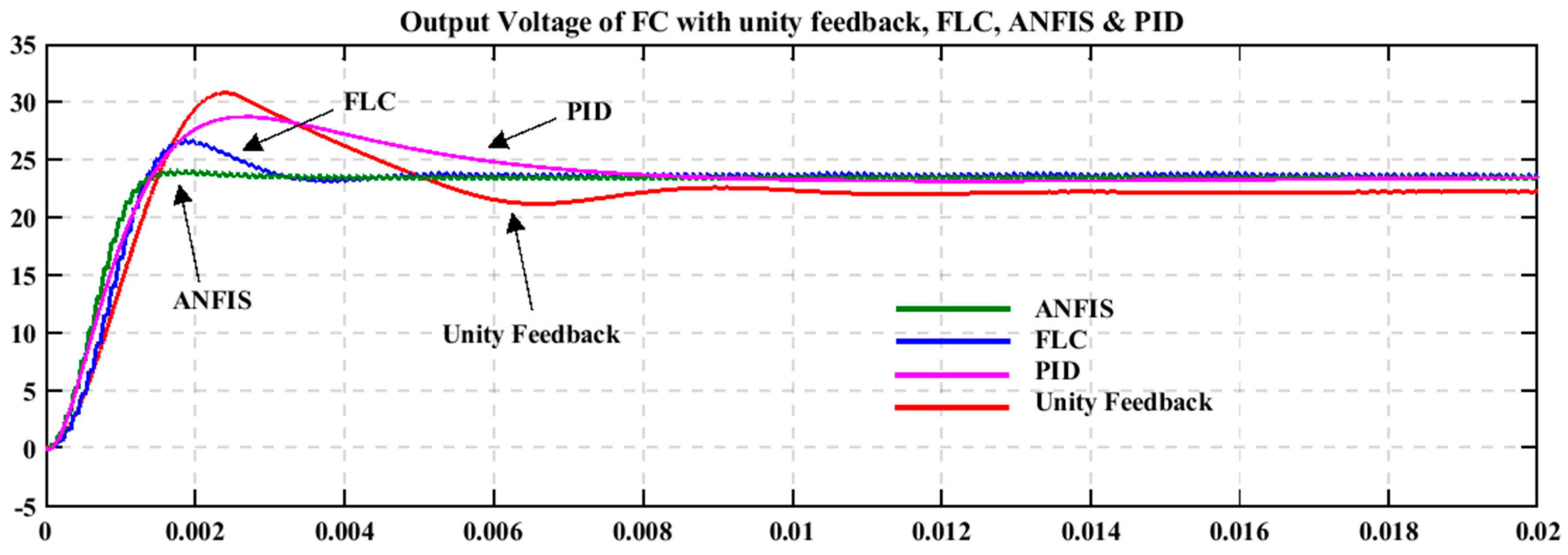
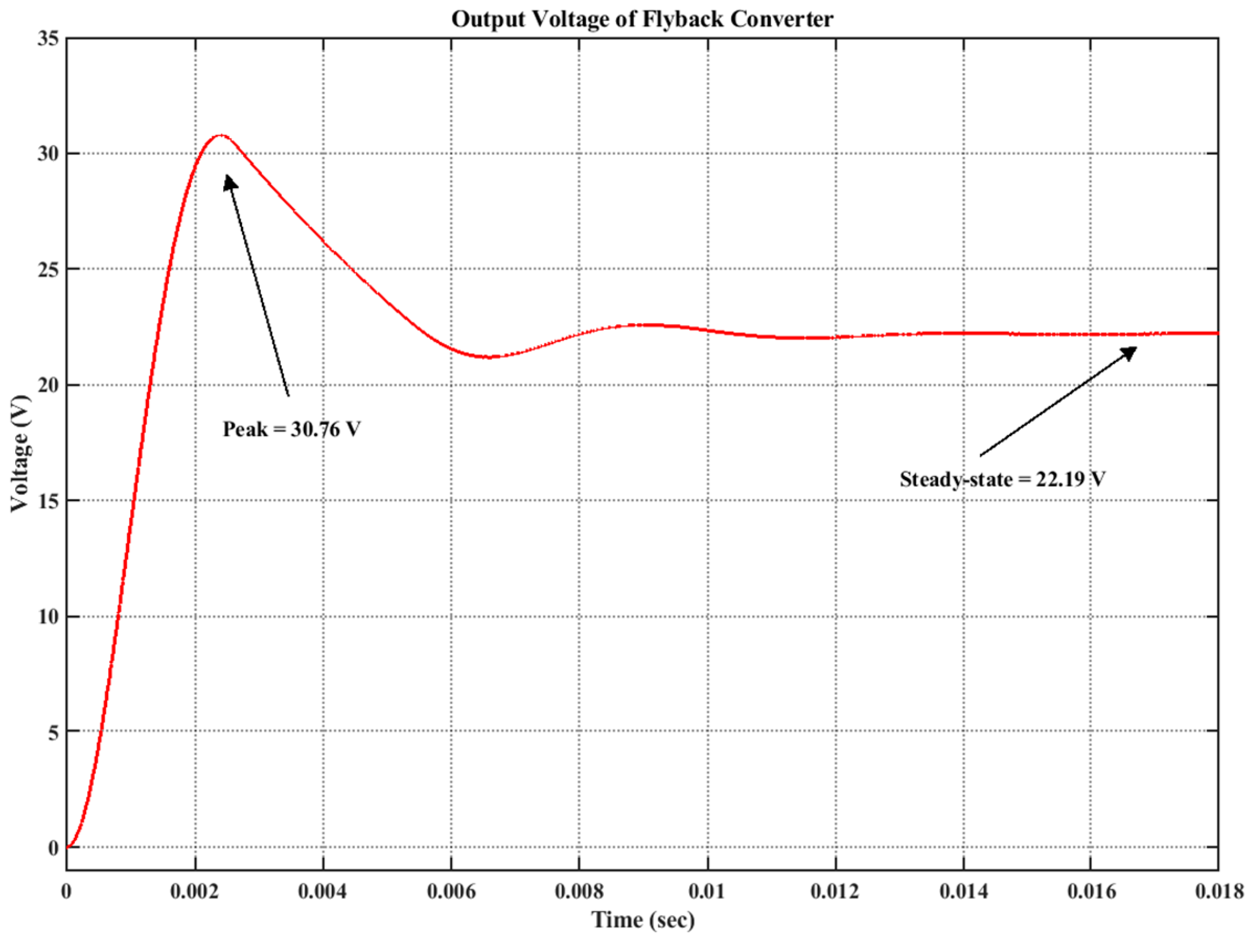
5.1. Nominal Performance

FC with unity feedback, FLC, ANFIS, and PID controllers were simulated for a fixed load. The output voltage offered by these controllers is shown in Figure 13. The PID parameters used were summarized in

Table 3. PID parameters.

PID Parameters	Values
Proportional gain KP	18.45
Integral gain KI	99,999.88
Derivative gain KD	0.00071

.

The response parameters extracted from Figure 13 are tabulated in

Table 4. Comparison of response parameters of unity feedback, FLC, ANFIS, and PID.

Parameters	Unity Feedback	FLC	ANFIS	PID
Rise time (ms)	1.0	0.8925	0.8827	0.98
Settling time (ms)	NaN	6.9	6.3	22.1
Overshoot (%)	28.1803	11.0875	0.5603	19.5644
Undershoot (%)	0.0022	0.0149	0.0205	0.3464
Peak (V)	30.7633	26.6610	24.1345	28.6955
Peak time (ms)	2.4	1.9	1.8	2.7
Steady-state error (%)	7.54	1.83	1.04	1.79

. From Table 4, it can be deduced that the ANFIS-based feedback controller had the least rise time, settling time, percentage overshoot, peak voltage, peak time, and steady-state error at 0.8827 ms, 6.3 ms, 0.5603%, 24.1345 V, 1.8 ms, and 1.04%, respectively, as compared to FLC and PID. Only the percentage undershoot was less, 0.0149%, in the case of FLC. The ANFIS controller completely outshone the other controllers.

5.2. Load Regulation

Load regulation was performed by changing the value of the load resistance and checking the capability of the controller to maintain a constant output voltage. For the load resistance change of 10 Ω to 14 Ω and from 10 Ω to 6 Ω, load current variations are shown in Figure 14. Reduced peak to peak voltage spike with reduced recovery time was observed at the time of load transience. The ANFIS controller offered excellent load regulation.

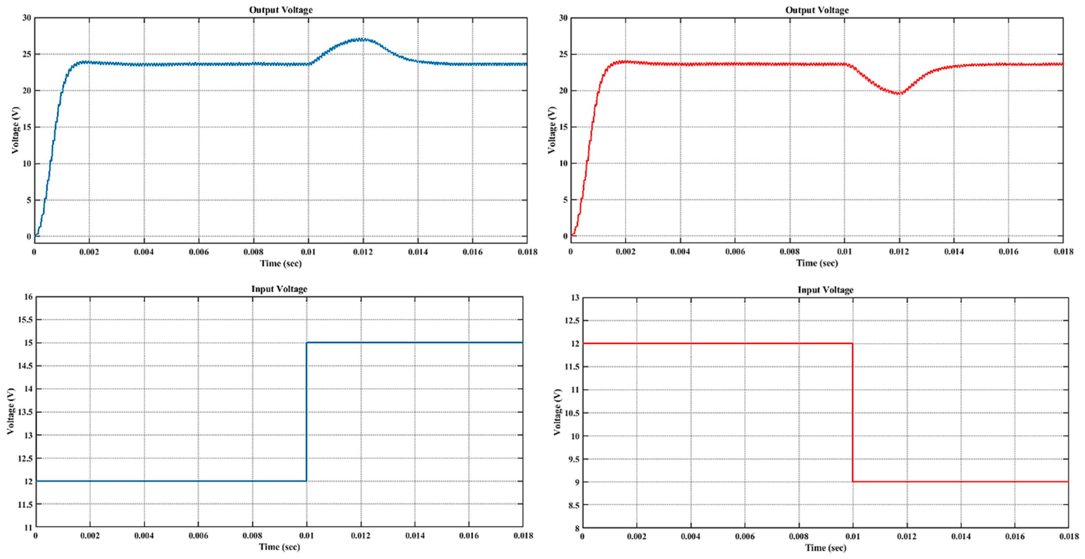
5.3. Line Regulation

Line regulation was performed by changing the value of the supply voltage and checking the capability of the controller to maintain a constant output voltage. The supply voltage was changed from 12 V to 15 V and 12 V to 9 V. The output voltage across the load resistance is presented in Figure 15. The controller was able to compensate for the changes in the supply voltage, thus offering superior line regulation.

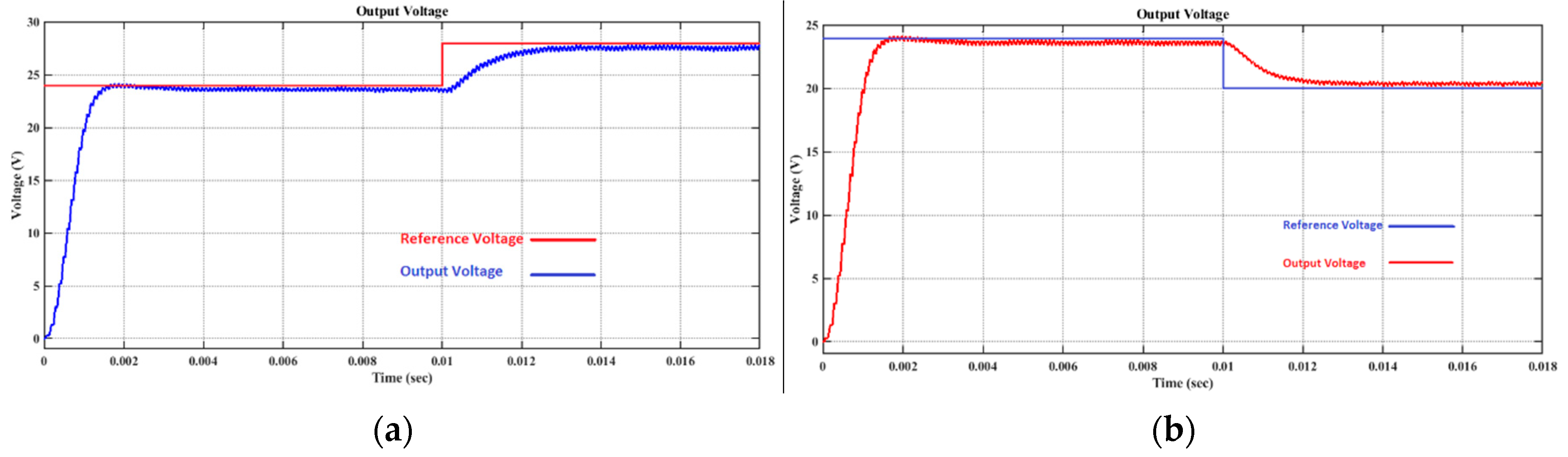
5.4. Change in Reference Voltage

The reference voltage was changed from 24 to 28 V. The output voltage waveform is presented in Figure 16a. Similarly, the reference voltage was changed from 24 to 20 V at time 0.01 s. The output voltage waveform is presented in Figure 16b. The output successfully followed the changes in the reference signal.

In a nutshell,

Table 5. Summarized results of (a) load regulation, (b) line regulation, and (c) change in the reference voltage.

(a)
Parameters	Step Load
	10 Ω to 14 Ω	10 Ω to 6 Ω
Load regulation (%)	0.31	0.65
Settling time (ms)	2.5	3.0
(b)
Parameters	Step Line
	12 V to 15 V	12 V to 9 V
Line regulation (%)	1.67	1.0
Settling time (ms)	5.5–6.0	5.5–6.0
(c)
Parameters	Reference Value Change
	24 V to 28 V	24 V to 20 V
Steady-state error (%)	0.9	1.05
Settling time (ms)	4.0–4.5	4.0–4.5

presents the complete summary of results related to line and load regulation and set-point tracking. The percentage load and line regulations were below 1%, except for the line regulation (when the input voltage was increased from 12 V to 15 V), i.e., 1.67%. The settling time for load regulation was less than the line regulation. The steady-state error, when the reference value changed, was also around 1% with settling times of approximately 4.0–4.5 ms.

6. Conclusions

To keep the output voltage of an FC system regulated as necessary for modern electronic devices irrespective of the changes in input voltage or load current, an ANFIS-based controller was proposed in this research. A FIS structure containing 25 fuzzy rules (in our case) relating the inputs and the output originally generated by the fuzzy logic system was tuned by ANFIS. It was observed that the FIS tuned by ANFIS exhibited better output voltage response under static and transient loads. Better set-point tracking was also achieved. ANFIS may utilize past results or experiences to make immediate decisions about the response. Training of fuzzy rules by ANFIS made the ANFIS-based controller more adaptive. Simulation results depicted that both the static and dynamic performance of the ANFIS-based controller was better in all aspects compared to the FLC and PID controllers. Hardware implementation of the proposed compensated system can be carried out in future.

References

1. Sarif, M.S.M.; Pei, T.X.; Annuar, A.Z. Modeling, design and control of bidirectional DC-DC converter using state-space average model. In Proceedings of the IEEE Symposium on Computer Applications & Industrial Electronics (ISCAIE), Penang, Malaysia, 28–29 April 2018; pp. 416–421. [Google Scholar]
2. Jiang, W.; Chincholkar, S.H.; Chan, C. Investigation of a Voltage-Mode Controller for a dc-dc Multilevel Boost Converter. IEEE Trans. Circuits Syst. II Express Briefs 2018, 65, 908–912. [Google Scholar] [CrossRef]
3. MShahid, A.; Yasin, A.R.; Ahmad, S. Practical sliding mode controller in Dc-Dc converters for use in hybrid vehicles. In Proceedings of the 19th International Multi-Topic Conference (INMIC), Islamabad, Pakistan, 5–6 December 2016; pp. 1–7. [Google Scholar]
4. Wang, C. A Novel ZCS-PWM Flyback Converter with a Simple ZCS-PWM Commutation Cell. IEEE Trans. Ind. Electron. 2008, 55, 749–757. [Google Scholar] [CrossRef]
5. Iqbal, H.K.; Abbas, G. Design and analysis of SMC for second order DC-DC flyback converter. In Proceedings of the 17th IEEE International Multi Topic Conference 2014, Karachi, Pakistan, 8–10 December 2014; pp. 533–538. [Google Scholar]
6. Tamyurek, B.; Torrey, D.A. A Three-Phase Unity Power Factor Single-Stage AC–DC Converter Based on an Interleaved Flyback Topology. IEEE Trans. Power Electron. 2011, 26, 308–318. [Google Scholar] [CrossRef]
7. Ohsato, T.; Satoh, N.; Sekiya, H. A flyback converter using power-MOSFETs to achieve high-frequency operation beyond 10MHz. In Proceedings of the IEEE 3rd International Future Energy Electronics Conference and ECCE Asia, Kaohsiung, Taiwan, 3–7 June 2017; pp. 1101–1105. [Google Scholar]
8. Xie, X.; Li, J.; Peng, K.; Zhao, C.; Lu, Q. Study on the Single-Stage Forward-Flyback PFC Converter With QR Control. IEEE Trans. Power Electron. 2016, 31, 430–442. [Google Scholar] [CrossRef]
9. Hwu, K.; Jiang, W. Isolated step-up converter based on flyback converter and charge pumps. IET Power Electron. 2014, 7, 2250–2257. [Google Scholar] [CrossRef]
10. Nymand, M.; Andersen, M.A.E. High-Efficiency Isolated Boost DC–DC Converter for High-Power Low-Voltage Fuel-Cell Applications. IEEE Trans. Ind. Electron. 2010, 57, 505–514. [Google Scholar] [CrossRef]
11. Yousefzadeh, V.; Shirazi, M.; Maksimovic, D. Minimum Phase Response in Digitally Controlled Boost and Flyback Converters. In Proceedings of the APEC—Twenty-Second Annual IEEE Applied Power Electronics Conference and Exposition, Anaheim, CA, USA, 25 February–1 March 2007; pp. 865–870. [Google Scholar]
12. Verma, S.; Singh, S.K.; Rao, A.G. Overview of control Techniques for FC-FC converter. Res. J. Eng. Sci. 2013, 2, 18–21. [Google Scholar]
13. Tan, S.; Lai, Y.M.; Tse, C.K.; Martinez-Salamero, L.; Wu, C. A Fast-Response Sliding-Mode Controller for Boost-Type Converters with a Wide Range of Operating Conditions. IEEE Trans. Ind. Electron. 2007, 54, 3276–3286. [Google Scholar] [CrossRef]
14. Salimi, M.; Soltani, J.; Zakipour, A.; Hajbani, V. Sliding mode control of the DC-DC flyback converter with zero steady-state error. In Proceedings of the 4th Annual International Power Electronics, Drive Systems and Technologies Conference, Tehran, Iran, 13–14 February 2013; pp. 158–163. [Google Scholar]
15. He, J.; Xu, J.; Yan, T. Peak current-controlled CRM flyback PFC converter with square of line voltage-compensated primary current envelope. Electron. Lett. 2015, 51, 684–686. [Google Scholar] [CrossRef]
16. Chandranadhan, V.R.; Renjini, G. Average current mode control of improved bridgeless flyback rectifier with bidirectional switch. In Proceedings of the International Conference on Circuits, Power and Computing Technologies [ICCPCT-2015], Nagercoil, India, 19–20 March 2015; pp. 1–6. [Google Scholar]
17. Park, J.; Moon, Y.J.; Jeong, M.G.; Kang, J.G.; Kim, S.H.; Gong, J.C.; Yoo, C. Quasi-Resonant (QR) Controller with Adaptive Switching Frequency Reduction Scheme for Flyback Converter. IEEE Trans. Ind. Electron. 2016, 63, 3571–3581. [Google Scholar] [CrossRef]
18. Chen, K.; Liang, T. Design of Quasi-resonant flyback converter control IC with DCM and CCM operation. In Proceedings of the International Power Electronics Conference, Hiroshima, Japan, 18–21 May 2014; pp. 2750–2753. [Google Scholar]
19. Dogra, A.; Pal, K. Designing and Tuning of PI Controller for Flyback Converter. Int. J. Eng. Trends Technol. (IJETT) 2014, 13, 117–122. [Google Scholar] [CrossRef]
20. Modak, S.; Panda, G.K.; Saha, P.K.; Das, S. Design of Novel Fly-Back Converter Using PID Controller. Int. J. Adv. Res. Electr. Electron. Instrum. Eng. 2015, 4, 289–297. [Google Scholar]
21. Priyadarshini, D.; Rai, S. Design, Modelling and Simulation of a PID Controller for Buck Boost and Cuk Converter. Int. J. Sci. Res. (IJSR) 2014, 3, 1226–1229. [Google Scholar]
22. Yilmaz, U.; Kircay, A.; Borekci, S. PV system flyback converter-controlled PI control to charge battery under variable temperature and irradiance. In Proceedings of the Electronics, Palanga, Lithuania, 19–21 June 2017; pp. 1–6. [Google Scholar]
23. Chen, T.H.; Lin, W.L.; Liaw, C.M. Dynamic modelling and controller design of flyback converter. IEEE Trans. Aerosp. Electron. Syst. 1999, 35, 1230–1239. [Google Scholar] [CrossRef]
24. Garcia-Rodriguez, L.A.; Williams, E.; Balda, J.C.; Gonzalez-Llorente, J.; Chiacchiarini, H. Control of a flyback converter operating in BCM using the natural switching surface. In Proceedings of the IEEE 6th International Symposium on Power Electronics for Distributed Generation Systems (PEDG), Aachen, Germany, 22–25 June 2015; pp. 1–8. [Google Scholar]
25. Chen, X.; Jiang, T.; Zhao, S.; Zeng, H.; Zhang, J. Evaluation of primary side control schemes for flyback converter with constant current output. In Proceedings of the Twenty-Eighth Annual IEEE Applied Power Electronics Conference and Exposition (APEC), Long Beach, CA, USA, 17–21 March 2013; pp. 1859–1863. [Google Scholar]
26. Singh, A.; Londhe, P.S. Design of signed distance method based fuzzy logic controller for TITO process. In Proceedings of the Recent Developments in Control, Automation & Power Engineering (RDCAPE), Noida, India, 26–27 October 2017; pp. 13–17. [Google Scholar]
27. Fahmizal; Kuo, C. Development of a fuzzy logic wall following controller for steering mobile robots. In Proceedings of the International Conference on Fuzzy Theory and Its Applications (iFUZZY), Taipei, Taiwan, 6–8 December 2013; pp. 7–12. [Google Scholar]
28. Deepa, K.; Jeyanthi, R.; Mohan, S.; Kumar, M.V. Fuzzy based flyback converter. In Proceedings of the International Conference on Advances in Electrical Engineering (ICAEE), Vellore, India, 9–11 January 2014; pp. 1–4. [Google Scholar]
29. Subbarao, M.; Babu, C.S.; Satyanarayana, S.; Kumar, S.L.V.S. Fuzzy controlled single stage AC/DC converter with PFC to drive LEDs. In Proceedings of the International Conference on Smart Electric Grid (ISEG), Guntur, India, 19–20 September 2014; pp. 1–5. [Google Scholar]
30. Kumar, P.R.; Kumar, S.L.V.S. Comparative Study of PID Based VMC and Fuzzy Logic Controllers for Flyback Converter. Int. J. Instrum. Control Autom. (IJICA) 2011, 1, 29–36. [Google Scholar]
31. Hamdan, H.; Garibaldi, J.M. Adaptive neuro-fuzzy inference system (ANFIS) in modelling breast cancer survival. In Proceedings of the International Conference on Fuzzy Systems, Barcelona, Spain, 18–23 July 2010; pp. 1–8. [Google Scholar]
32. Hosseini, S.A.; Afrakoti, I.E.P. Evaluation of a new neutron energy spectrum unfolding code based on an Adaptive Neuro-Fuzzy Inference System (ANFIS). J. Radiat. Res. 2018, 59, 436–441. [Google Scholar] [CrossRef]
33. Zhai, J.; Zhou, J.; Zhang, L.; Zhao, J.; Hong, W. Dynamic Behavioral Modeling of Power Amplifiers Using ANFIS-Based Hammerstein. IEEE Microw. Wirel. Compon. Lett. 2008, 18, 704–706. [Google Scholar] [CrossRef]
34. Farayola, A.M.; Hasan, A.N.; Ali, A. Curve fitting polynomial technique compared to ANFIS technique for maximum power point tracking. In Proceedings of the 8th International Renewable Energy Congress (IREC), Amman, Jordan, 21–23 March 2017; pp. 1–6. [Google Scholar]
35. Mohammed, S.S.; Devaraj, D.; Ahamed, T.P.I. Maximum power point tracking system for standalone solar PV power system using Adaptive Neuro-Fuzzy Inference System. In Proceedings of the Biennial International Conference on Power and Energy Systems: Towards Sustainable Energy (PESTSE), Bangalore, India, 21–23 January 2016; pp. 1–4. [Google Scholar]
36. Chu, Y.; Yuan, L.; Chiang, H. ANFIS-based maximum power point tracking control of PV modules with DC-DC converters. In Proceedings of the 18th International Conference on Electrical Machines and Systems (ICEMS), Pattaya, Thailand, 25–28 October 2015; pp. 692–697. [Google Scholar]
37. Tarek, B.; Said, D.; Benbouzid, M.E.H. Maximum Power Point Tracking Control for Photovoltaic System Using Adaptive Neuro-Fuzzy ANFIS. In Proceedings of the Eighth International Conference and Exhibition on Ecological Vehicles and Renewable Energies (EVER), Monte Carlo, Monaco, 27–30 March 2013; pp. 1–7. [Google Scholar]
38. Noman, A.M.; Addoweesh, K.E.; Alolah, A.I. Simulation and Practical Implementation of ANFIS-Based MPPT Method for PV Applications Using Isolated Ćuk Converter. Int. J. Photoenergy 2017, 2017, 3106734. [Google Scholar] [CrossRef]
39. Al-Nussairi, M.K.; Bayindir, R.; Hossain, E. Fuzzy logic controller for Dc-Dc buck converter with constant power load. In Proceedings of the IEEE 6th International Conference on Renewable Energy Research and Applications (ICRERA), San Diego, CA, USA, 5–8 November 2017; pp. 1175–1179. [Google Scholar]
40. Feng, G. A Survey on Analysis and Design of Model-Based Fuzzy Control Systems. IEEE Trans. Fuzzy Syst. 2006, 14, 676–697. [Google Scholar] [CrossRef]
41. Swathy, M.K.; Jantre, M.S.; Jadhav, M.Y.; Labde, M.S.M.; Kadam, M.P. Design and Hardware Implementation of Closed Loop Buck Converter Using Fuzzy Logic Controller. In Proceedings of the Second International Conference on Electronics, Communication and Aerospace Technology (ICECA), Coimbatore, India, 29–31 March 2018; pp. 175–180. [Google Scholar]
42. Bendaoud, K.; Krit, S.; Kabrane, M.; Ouadani, H.; Elaskri, M.; Karimi, K.; Elbousy, H.; Elmaimouni, L. Fuzzy logic controller (FLC): Application to control DC-DC buck converter. In Proceedings of the International Conference on Engineering & MIS (ICEMIS), Monastir, Tunisia, 8–10 May 2017; pp. 1–5. [Google Scholar]
43. de Martins, J.K.E.C.; de Araújo, F.M.U. Nonlinear system identification based on modified ANFIS. In Proceedings of the 12th International Conference on Informatics in Control, Automation and Robotics (ICINCO), Colmar, France, 21–23 July 2015; pp. 588–595. [Google Scholar]
44. García, P.; García, C.A.; Fernández, L.M.; Llorens, F.; Jurado, F. ANFIS-Based Control of a Grid-Connected Hybrid System Integrating Renewable Energies, Hydrogen and Batteries. IEEE Trans. Ind. Inform. 2014, 10, 1107–1117. [Google Scholar] [CrossRef]
45. Al-Hmouz, A.; Shen, J.; Al-Hmouz, R.; Yan, J. Modeling and Simulation of an Adaptive Neuro-Fuzzy Inference System (ANFIS) for Mobile Learning. IEEE Trans. Learn. Technol. 2012, 5, 226–237. [Google Scholar] [CrossRef]
46. Hiremath, S.; Patra, S.K. Transmission rate prediction for Cognitive Radio using Adaptive Neural Fuzzy Inference System. In Proceedings of the 5th International Conference on Industrial and Information Systems, Mangalore, India, 29 July–1 August 2010; pp. 92–97. [Google Scholar]
47. Sowmmiya, U.; Uma, G. ANFIS-based sensor fault-tolerant control for hybrid grid. IET Gener. Transm. Distrib. 2018, 12, 31–41. [Google Scholar] [CrossRef]
48. Ying, L.; Pan, M. Using adaptive network based fuzzy inference system to forecast regional electricity loads. Energy Convers. Manag. 2008, 49, 205–211. [Google Scholar] [CrossRef]
49. Abbas, G.; Muazzam, H.; Farooq, U.; Gu, J.; Asad, M.U. Comparative Analysis of Analog Controllers for DC-DC Buck Converter. J. Autom. Control Eng. 2015, 3. [Google Scholar] [CrossRef]
Figure 1. Block diagram of the complete system.
Applsci 09 05108 g001
Figure 2. The output of FC with unity feedback.
Applsci 09 05108 g002
Figure 3. Fuzzy logic controller (FLC) block diagram.
Applsci 09 05108 g003
Figure 4. FC model with FLC in MATLAB/Simulink.
Applsci 09 05108 g004
Figure 5. MFs of (a) input variable error e, (b) input variable Δe, and (c) output variable duty cycle d.
Applsci 09 05108 g005
Figure 6. Rules representation by the 3D surface view.
Applsci 09 05108 g006
Figure 7. Adaptive neuro-fuzzy inference system (ANFIS) general architecture with two inputs (with five membership functions for each input), one output, and 25 rules.
Applsci 09 05108 g007
Figure 8. Flowchart of implementation of ANFIS.
Applsci 09 05108 g008
Figure 9. Loading of training data into the neuro-fuzzy designer.
Applsci 09 05108 g009
Figure 10. Comparison of training data and output FIS after training.
Applsci 09 05108 g010
Figure 11. Neural network diagram.
Applsci 09 05108 g011
Figure 12. New rules surface, after training in ANFIS.
Applsci 09 05108 g012
Figure 13. The output voltage of FC with unity feedback, FLC, ANFIS, and proportional–integral–derivative (PID) controllers.
Applsci 09 05108 g013
Figure 14. Output voltage and load current when the load resistance was (a) increased and (b) decreased.
Applsci 09 05108 g014
Figure 15. Output voltage and load current when the input voltage was increased and decreased.
Applsci 09 05108 g015
Figure 16. Output voltage when the reference voltage was (a) increased and (b) decreased.
Applsci 09 05108 g016