A Head Control Strategy of the Snake Robot Based on Segmented Kinematics

Abstract

Head control is important for snake robots to work in an unknown environment. However, the existing methods of head control have certain application limitations for snake robots with different configurations. Thus, a strategy for head control based on segmented kinematics is proposed. Compared with the existing head control strategies, our strategy can adapt to different structures of snake robots, whether wheeled or non-wheeled. In addition, our strategy can realize the accurate manipulation of the snake robot head. The robot body is divided into the base part, neck part and head part. First, parameters of backbone curve are optimized for enlarging the area of the support polygon. Then the desired pose for the head link and the dexterous workspace of the head part can in turn derive the desired position and direction of the end frame for the neck part. An optimization algorithm is proposed to help the end frame of the neck part approach a desired one and obtains the joint angles of the neck part. When the actual frames of the neck part are determined, the dexterous workspace of the head part will cover the desired pose of the head link. Then the TRAC-IK inverse kinematics algorithm is adopted to solve the joint angles of the head part. To avoid the collision between the body and the ground, a trajectory planning method of the overall body in Cartesian space is proposed. Finally, simulations validate the effectiveness of the control strategy.

1. Introduction

Snake robots can adapt to complex environments and move flexibly because of their hyper-redundancy degrees of freedom (DOFs) [1,2,3,4]. However, it needs to obtain information about the surrounding environment if a snake robot wants to work well in a complex environment. Several researchers equip the head of the snake robot with a small camera [5,6]. The desired image information is needed to obtain from the head camera. Moreover, we need to move the head of the snake robot to a specific position and make it as a manipulator in some scenes. Then the head control strategy of the snake robot is required.

Tanaka et al. proposed the algorithm of head control for the planar snake robot [7] and realized the control of the movement direction of the snake robot head on a plane. Then they further proposed a new head control algorithm in a three-dimensional space by using kinematic redundancy [8]. However, these algorithms are based on the assumption of the velocity constraint, and the assumption is only suitable for the snake robot with wheels. However, snake robots without wheels are also widely studied, and they are more flexible and more adaptable to complex environments than ones with wheels. Ye et al. proposed a head control method of the snake robot based on the serpenoid curve [9], and then they used the zero-moment point (ZMP) method to analyze the stability of the motion of the snake robot. Zhang et al. proposed a predefined spiral curve method to control the head of the snake robot [10]. The method is implemented on the snake robot with 3 degrees of freedom joints. However, the predefined spiral curve method limits the range of motion of the head to a certain extent. Moreover, it is not adapted well to these snake robots with single DOF or two DOFs joints. In addition, the method based on serpenoid curve and the predefined spiral curve method cannot achieve control of the arrival of the head of the snake robot to a specific position and posture.

To solve these problems, a strategy of the head control of the snake robot based on segmented kinematics is proposed, and it uses the optimization algorithm to enhance the stability of its motion. Moreover, it can give the solution of the joint angles for the specific pose of the head of the robot. In addition, it also solves the problem of the trajectory planning of the overall body for the snake robot.

To realize the control strategy, the base part is controlled by the method of discretizing the backbone curve. The specific structure of the snake robot used in this paper is shown in Figure 1. The backbone curve theory is proposed by Chirikjian et al. [11]. In addition, then the backbone curve discretization method is adopted widely [12,13]. For enhancing the motion stability of the overall body, the backbone curve is designed as a plane arc and the parameters of the arc are also optimized. For the neck part of the robot, we need to determine the desired position and direction of the end link of the neck part by the dexterous workspace of the head part and the desired pose of the head. The method of calculating the dexterous workspace is introduced in the literature [14]. Once the desired position and direction of the end link of the neck part are determined, the optimization algorithm can calculate the joint angles of the neck part. Then the end frame (the frame of the end link) of the neck part is treated as the base frame of the head part, and an inverse kinematics algorithm is selected to solve the joint angles of the head part. Now there are several inverse kinematics algorithms, such as the KDL algorithm [15,16], the inverse kinematics algorithm based on the optimization [17] and TRAC-IK algorithm [18]. The TRAC-IK algorithm is adopted for its better efficiency and high solution rate. Then all the joint angles of the snake robot are obtained. However, the snake robot will hit the ground if only the trajectory planning in joint space is considered. Thus, a trajectory planning method of the overall body in Cartesian space is proposed. The stability of the motion is analyzed by the support polygon method and the zero-moment point method.

Compared with the existing head control strategies, our proposed strategy has some advantages. Tanaka et al. proposed the head control strategies of the wheeled snake robot on a plane or in a three-dimensional space [7]. However, these strategies are both based on the non-side slip constraint, and they are hard to be applied to the non-wheeled snake robot. Our proposed strategy can be applied to snake robots and non-wheeled snake robots. Moreover, the strategies proposed by Zhang and Ye are hard to realize the accurate manipulation of the snake robot head since they are both based on the gait or the pure backbone curve of snake robots [9,10]. However, our proposed strategy can realize the accurate manipulation of the head since it adopts segmented kinematics. In addition, the trajectory planning of the overall body in Cartesian space is proposed to avoid the collision with the ground.

The article is organized as follows. The strategy of head control is introduced in the Section 2. The strategy includes the calculation of joint angles for the base part, the calculation of the dexterous workspace of the head part, choosing the dexterous workspace center and the calculation of joint angles for the neck part. The description of the process of head control is in Section 3. The stability analysis methods of the motion are given, and the trajectory planning method of the overall body is proposed in this section. In Section 4, the simulations of catching the spheres and getting through a hole on the wall are shown. In the Section 5, the discussions and conclusions are given.

2. The Strategy of the Head Control

The strategy of the head control is segmented, and it is divided into the calculations of the joint angles for the base part, the neck part and head part. The joint angles of the base part are obtained by discretizing the backbone curve of the base part. For the neck part, the desired pose for the head link and the dexterous workspace of the head part can in turn derive a desired position and direction of the end frame of the neck part. The joint angles are determined by making the end frame of the neck part approach the desired one. Thus, the dexterous workspace and the center of the dexterous workspace of the head part are needed. Once the neck part is determined, the end frame of the neck part is used for the base frame of the head part. The joint angles of the head part can be solved by the inverse kinematics algorithm.

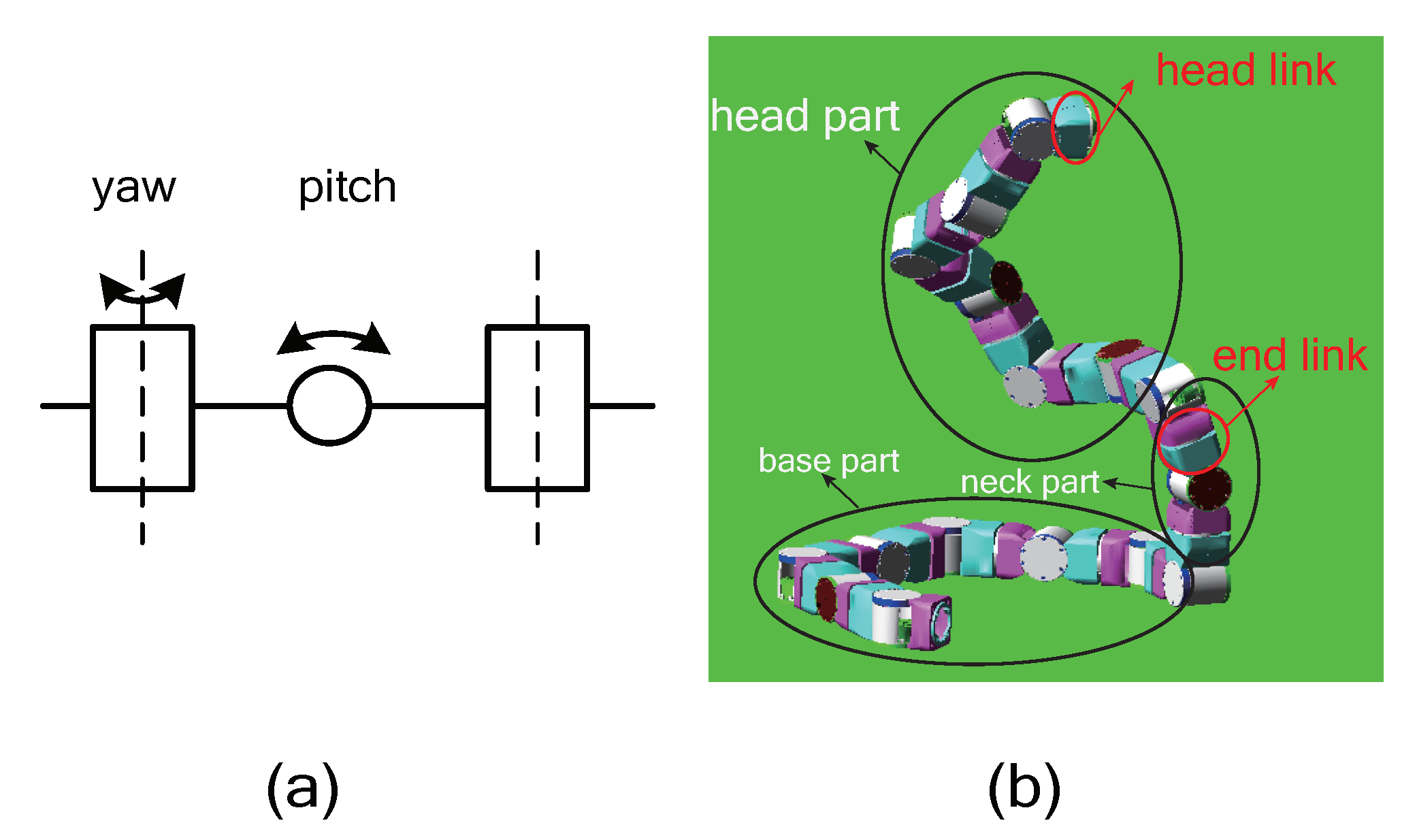
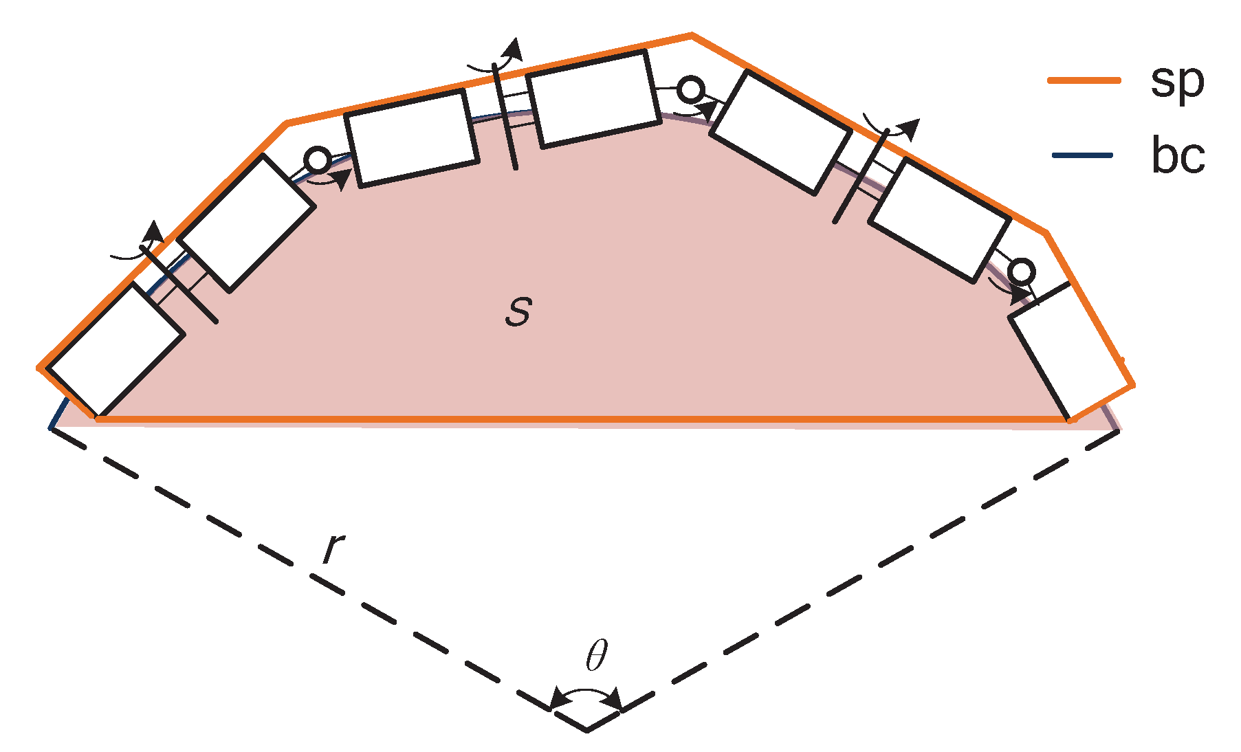
2.1. The Calculation of Joint Angles for the Base Part

In this paper, the axis of the snake robot is orthogonal to each other and the joint has only one degree of freedom. This structure is widely adopted by the researcher in the snake robot field [5,19,20]. The illustration of the snake robot configuration can be seen in Figure 1a. The robot has two types of joints, the yaw joint and the pitch joint. This configuration can help the snake robot to achieve motion in three-dimensional space. The base part of the robot is the part contacting with the ground, which is shown in Figure 1b.

In the process of the head control for the snake robot, the base part is used to ensure the body of the snake robot keeps stable. The support polygon method and zero-moment point method are usually used to judge whether the body is stable [21]. When the support polygon has a larger area, the body will have a greater possibility of stable standing. As we know, for a given perimeter of the polygon, the circle has the largest coverage area among all the plane polygons. Thus, we design the backbone of the base part as a plane circle. Then we use the backbone curve theory to discretize the backbone curve to generate the joint angles of the base part. The support polygon and the backbone curve are shown in Figure 2.

We assume that the backbone curve of the base part has a length l, and the joint angles of the base part are generated by the discretizing a plane arc with a radius r. Thus, we have the following equations,

$$r=\frac{l}{\theta }$$

(1)

$$S=\frac{1}{2}{r}^2(\theta -sin\left(\theta \right))$$

(2)

where $\theta$ is the central angle of the plane arc, and S is the area enclosed by the backbone curve, shown in Figure 2. When $\theta$ equals $\pi$, S have the maximum value $1/2\pi r^2$. More details about the support polygon and zero-moment point will be introduced in Section 3.

After the backbone curve of the base part is determined, we need to discretize the backbone curve to obtain joint angles. We adopt the discretization method based on the curvature and torsion of the backbone curve [22]. The corresponding formulas are given as:

$$\varphi ={\int }_0^s\tau \left(s\right)\mathrm{d}s$$

(3)

$$\left\{\begin{array}{c}{\kappa }_y\left(s\right)=\kappa \left(s\right)cos\left(\varphi \right)\hfill \\ {\kappa }_p\left(s\right)=\kappa \left(s\right)sin\left(\varphi \right)\hfill \end{array}\right.$$

(4)

$${\theta }_y={\int }_{s_1}^{s_2}{k}_y\left(s\right)\mathrm{d}s$$

(5)

$${\theta }_p={\int }_{s_1}^{s_2}{k}_p\left(s\right)\mathrm{d}s$$

(6)

where $\kappa \left(s\right)$ and $\tau \left(s\right)$ are the curvature and the torsion of the backbone curve at the arc length s. $\varphi$ is the phase angle of the discretization. In addition, it is obtained by the integral of the torsion on the arc length s. In addition, it describes the twist of the Frenet–Serret frame along the backbone curve [23]. ${\kappa }_y$ and ${\kappa }_p$ are the curvature projection on the yaw direction and the pitch direction, which are used to describe the bending along the yaw and pitch direction. Furthermore, ${\theta }_y$ and ${\theta }_p$ are the yaw joint angles and the pitch joint angles of the base part shown in the Figure 1a. $s_2$ and $s_1$ in Equations (5) and (6) are the start arc length and end arc length of the discretization respectively. For a spatial curve $\mathit{r}\left(t\right)$, its curvature $\kappa$ and torsion $\tau$ can be calculation as [23]:

$$\left\{\begin{array}{c}\kappa =\frac{|{\mathit{r}}^{\prime }\times {\mathit{r}}^{″}|}{|{\mathit{r}}^{\prime }{|}^3}\hfill \\ \tau =\frac{({\mathit{r}}^{\prime }\times {\mathit{r}}^{″})·{\mathit{r}}^{‴}}{|{\mathit{r}}^{\prime }\times {\mathit{r}}^{″}{|}^2}\hfill \end{array}\right.$$

(7)

where ${\mathit{r}}^{\prime }$, ${\mathit{r}}^{″}$ and ${\mathit{r}}^{‴}$ are the first, second and third order derivatives of $\mathit{r}$ to the general parameter t, respectively.

For the plane arc, it has the curvature $\kappa =\frac{1}{r}$ and torsion $\tau =\frac{}{}0$. In addition, Equations (4)–(6) can be simplified to

$$\left\{\begin{array}{c}{\kappa }_y=\kappa \left(s\right)\hfill \\ {\kappa }_p=0\hfill \end{array}\right.$$

(8)

$$\left\{\begin{array}{c}{\theta }_y={\kappa }_y\mathsf{\Delta }s\hfill \\ {\theta }_p=0\hfill \end{array}\right.$$

(9)

where $\mathsf{\Delta }s=s_2-s_1$. In addition, substitute $\kappa =\frac{1}{r}$ into Equation (9), the result that ${\theta }_y=\frac{\mathsf{\Delta }s}{r}$ is obtained. The discretization result of the plane arc is shown in Figure 3.

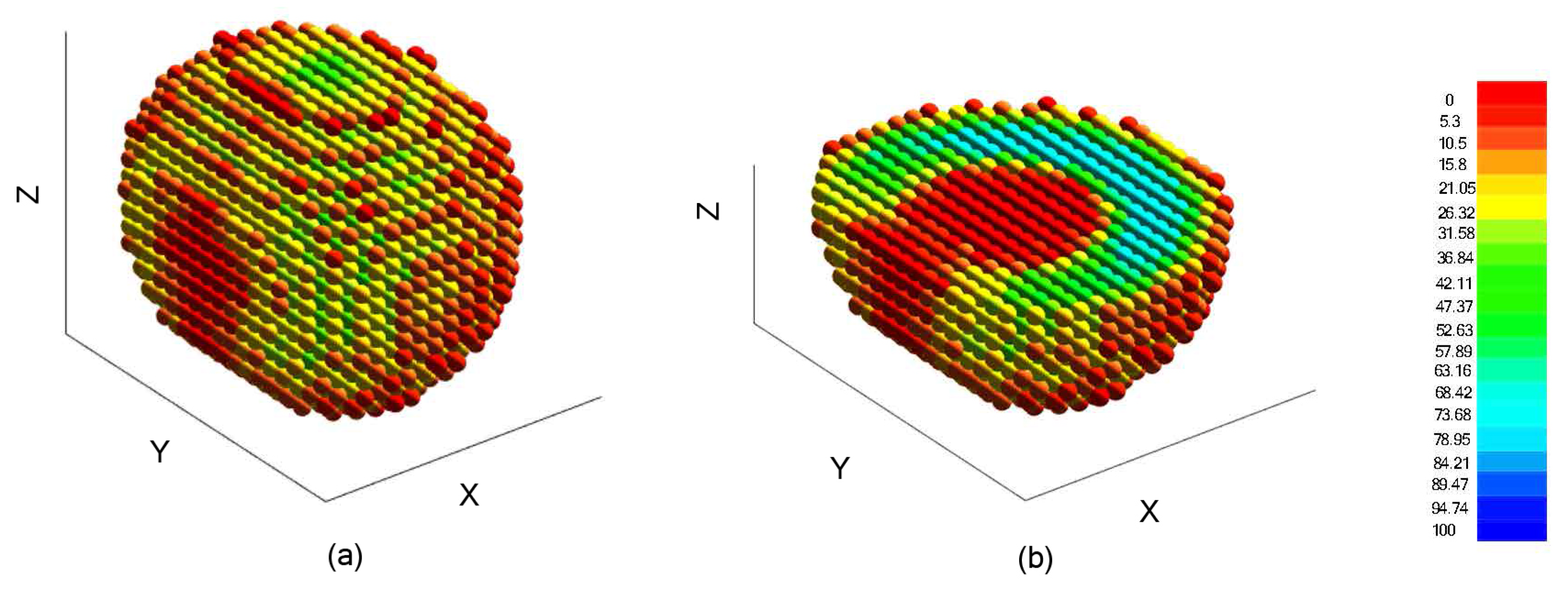
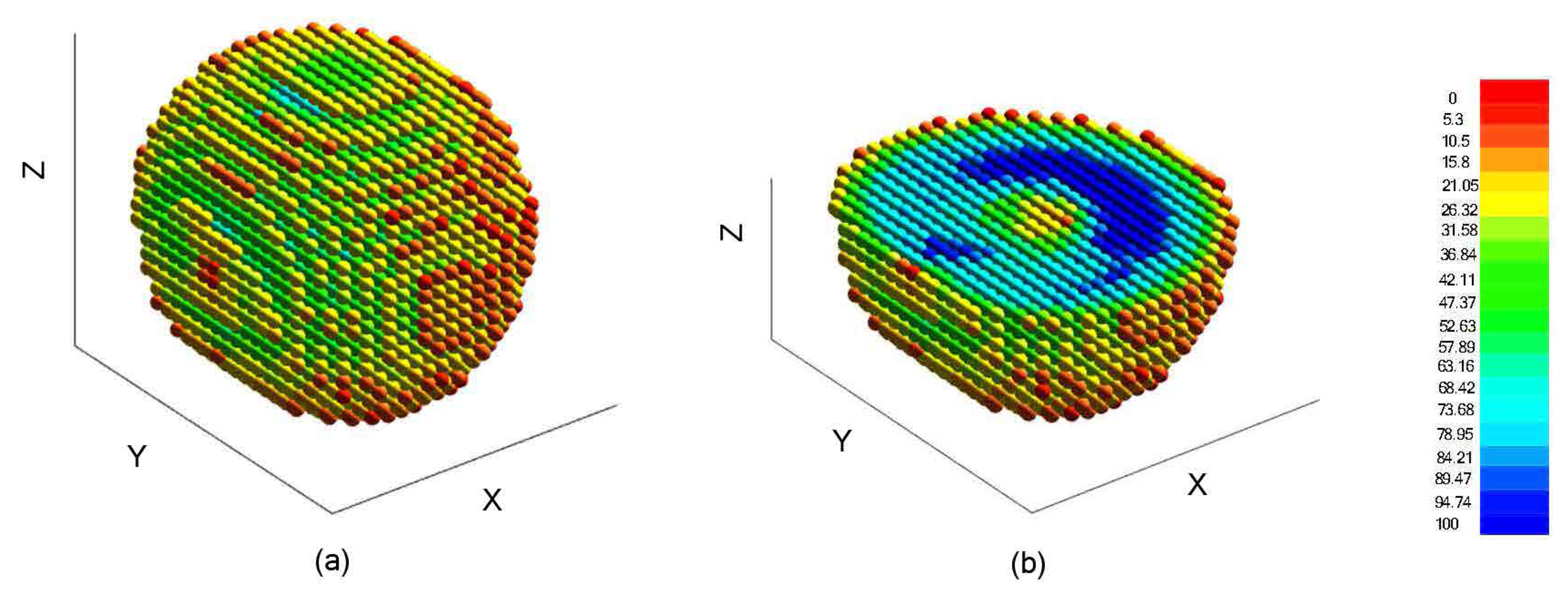
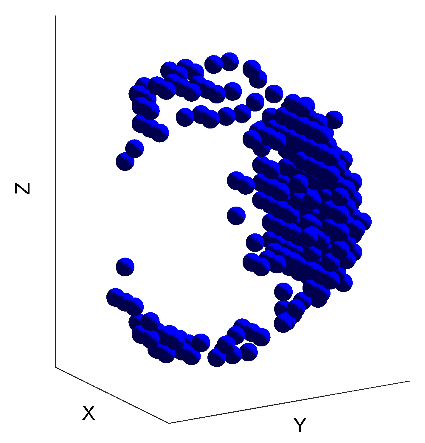
2.2. The Workspace of Head Part

To simplify the control of the snake robot and ensure the head of the snake robot can achieve the desired position and posture, we consider the head part has six or seven DOFs. Furthermore, the head of the snake robot can approach it if the workspace of the head part can cover the desired pose. Then the joint angles of the head part can be determined. To get the workspace of the head part of the snake robot, we need a reliable inverse kinematics algorithm. Aim to get the ability of motion in the 3-dimension space and imitate the biological snake, the snake robot has the configuration that the joint axes are orthogonal to each other. However, the inverse kinematics of the head part with six or seven DOFs has no analytical solution for this configuration.

Then some numerical algorithms such as the KDL algorithm [15,16], the inverse kinematics algorithm based on optimization [17] and TRAC-IK algorithm [18], are chosen.

For the KDL algorithm, it is a feedback and iteration process. (1) Forward Kinematics is used to compute the current pose of the end effector in the Cartesian space through the current joint angles ${\mathit{q}}_0$, (2) the linear interpolation method and the spherical linear interpolation method are used for the interpolation of the Cartesian position and the orientation represented by the unit quaternion and the desired linear velocity ${\mathit{v}}_d$ and angular velocity ${\mathit{\omega }}_d$ can be obtained, (3) the error ${\mathit{E}}_p$ between the desired pose and the current pose of the end effector is calculated, ${\mathit{E}}_p=[{\mathit{e}}_p,{\mathit{e}}_o]$, where ${\mathit{e}}_p$ and ${\mathit{e}}_o$ represent the position and orientation error of the end effector, (4) the inverse of the Jacobian, ${\mathit{J}}^{-1}$ convert the velocity of the end effector to the joint angular velocity. The equations used in the KDL iteration algorithm is given [16],

$${\dot{\mathit{q}}}_{m-1}={\mathit{J}}^{-1}\left({\mathit{q}}_{m-1}\right)\left(\begin{array}{c}{\mathit{v}}_d+{\mathit{K}}_p{\mathit{e}}_p\\ {\mathit{\omega }}_d+{\mathit{K}}_o{\mathit{e}}_o\end{array}\right)$$

(10)

$${\mathit{q}}_m={\mathit{q}}_{m-1}+{\dot{\mathit{q}}}_{m-1}\mathsf{\Delta }t$$

(11)

$${\mathit{e}}_p={\mathit{p}}_d-{\mathit{p}}_e\left({\mathit{q}}_m\right)$$

(12)

$${\mathit{e}}_o={\eta }_e\left({\mathit{q}}_m\right){\mathit{ϵ}}_d-{\eta }_d{\mathit{ϵ}}_e\left({\mathit{q}}_m\right)-{\mathit{ϵ}}_d\times {\mathit{ϵ}}_e\left({\mathit{q}}_m\right)$$

(13)

where ${\mathit{p}}_d$ and ${\mathit{p}}_e\left({\mathit{q}}_m\right)$ are the desired position and the calculated position of the end effector, respectively. $\{{\eta }_d,{\mathit{ϵ}}_d\}$ and $\{{\eta }_e,{\mathit{ϵ}}_e\}$ are the desired orientation and computed orientation of the end effector represented by the unit quaternion, respectively. ${\mathit{K}}_p$ and ${\mathit{K}}_o$ are gain matrices, which are $n\times n$ diagonal matrices. They should be selected properly to avoid the divergence of the iteration process. m represents the times of the iteration. When ${\mathit{E}}_p\approx 0$, the iteration of the algorithm stops, and the result is output. However, result of the joint angle is usually beyond the joint limit though the classical avoiding joint limit method, the gradient projection method is adopted [24]. Moreover, the KDL method is also easily stuck in the local minima. For the configuration of the head part with 6 DOFs, KDL algorithm has 62.9% solve rate. For the configuration of the head part with 7 DOFs, KDL algorithm has 73.5% solve rate. The desired pose sample size and current pose sample size are both 1000 samples generated by the random joint angles within the joint limit.

For the inverse kinematics algorithm based on the optimization, it can guarantee that the joint angles are within the joint limit. At first, we need to consider an objective function [17],

$$\begin{array}{cc}\hfill arg\underset{\mathit{q}\in {\mathbb{R}}^n}{min}& \mathrm{sumsqr}({\left[\begin{array}{ccc}{\mathit{R}}_d& & {\mathit{p}}_d\\ \mathbf{0}& & 1\end{array}\right]}^{-1}\mathit{f}\left(\mathit{q}\right)-k\mathit{I})\hfill \\ \hfill & s.t.q_i\le q_{\lim }^i,i=1,2,3,\dots ,n\hfill \end{array}$$

(14)

$$\mathit{f}\left(\mathit{q}\right)={}^0{\mathit{T}}_1{}^1{\mathit{T}}_2\cdots {}^{n-1}{\mathit{T}}_n$$

(15)

where ${\mathit{R}}_d$ is the $3\times 3$ rotation matrix, which represents the desired orientation. In addition, ${\mathit{p}}_d$ is the desired position vector. $\mathit{f}\left(\mathit{q}\right)$ is a function of the forward kinematics with joint angle vector $\mathit{q}$, which is used to obtain the transformation matrix of the end effector of the robot described in the world frame. The symbol ${}^{n-1}{\mathit{T}}_n$ indicates the transformation matrix of the n-th link relative to the $(n-1)$-th link. In addition, the frame 0 represent the world frame in Equation (15). $\mathit{I}$, k and $q_{\lim }^i$ are an identity matrix, a gain coefficient and the joint limit of the i-th joint, respectively. Function $\mathrm{sumsqr}$ calculates sum of squared elements of the input matrix. For the nonlinear optimization problem, the active-set algorithm, SQP algorithm and interior-point algorithm can be selected [25]. For the configuration of the head part with 6 DOFs, the active-set algorithm, the interior-point algorithm and the SQP algorithm have 57.7%, 67.5% and 61.1% solve rate, respectively. For the configuration of the head part with 7 DOFs, the active-set algorithm, the interior-point algorithm and the SQP algorithm have 59.8%, 77.1% and 65.8% solve rate, respectively. The desired pose sample size and current pose sample size are both 1000 samples generated by the random joint angles within the joint limit, respectively. However, the optimization algorithm is difficult to guarantee that it always has global convergence.

For the TRAC-IK inverse kinematics algorithm [18], the random restart of KDL called KDL-RR is used to solve the problem that it is stuck in local minima. TRAC-IK spawns the KDL-RR and SQP optimization inverse kinematics solver at the same time and run them for solving the inverse kinematics. The TRAC-IK solver will stop when either of the two solvers finishes with a solution or both exceed the set run time. The TRAC-IK enlarges the solution rate and shortens the solution time. For the configuration of the head part with 6 DOFs, TRAC-IK algorithm has 99.8% solve rate. For the configuration of the head part with 7 DOFs, TRAC-IK algorithm has 99.3% solve rate. The desired pose sample size and current pose sample size are also both 1000 samples generated by the random joint angles within the joint limit.

By comparing the above results, we chose the TRAC-IK algorithm to calculate the workspace for the head part. The specific calculation method of the workspace is introduced in the literature [14]. However, for the heart part, as we know, it needs to have at least six DOFs to reach a specific pose. For simplifying the control of the head, we decide that the head part has six or seven DOFs. Then we calculate the workspace of the head part with a reachability measure. The algorithm is shown in Algorithm 1, and the symbols in Algorithm 1 are shown in

Table 1. The symbols of Algorithm 1.

Symbol	Description
$\mathrm{fkine}\left(\mathit{x}\right)$	calculate the forward kinematics using joint angles $\mathit{x}$.
$\mathrm{boundary}\left(\mathit{x}\right)$	extracts the space boundary face of point group $\mathit{x}$.
$\mathrm{convex}\left(\mathit{x}\right)$	build a polyhedron based on the boundary $\mathit{x}$.
$\mathrm{innerSphere}\left(x\right)$	build an inscribed sphere of the box x.
$\mathrm{distribute}\left(x\right)$	distribute a certain number of points evenly on the sphere x.
$\mathrm{frame}\left(\mathit{p}\right)$	build a frame with an origin $\mathit{p}$, and z-axis is unit vector from the center of the sphere to $\mathit{p}$. X-axis and y-axis build a plane tangent to the sphere and obey right-hand law.
$\mathrm{rotFrame}\left({\mathit{f}}_r\right)$	rotate frame ${\mathit{f}}_r$ along its Z-axis to generate several frames evenly in a range of 360 degree.
$\mathrm{addPosition}(\mathit{rotF},\mathit{p})$	add a position vector $\mathit{p}$ to a rotation matrix $\mathit{rotF}$ and build a transformation matrix $\mathit{T}$.
$\mathrm{TRAC}-\mathrm{IK}\left(\mathit{T}\right)$	use TRAC-IK algorithm to solve the transformation matrix $\mathit{T}$.
$L_i$	the link length of the i-th link for the head part.
${\mathit{O}}_{base}$	the origin of the base frame for the head part.

.

Through Algorithm 1, we calculate the reachability of the workspace of the head part with 7 DOFs and 6 DOFs, respectively. The workspace is calculated in the base frame of the head part. The reachability of the workspace with 6 DOFs is shown in Figure 4. The reachability of the workspace with 7 DOFs is shown in Figure 5. The gradient color from red to blue indicates that the reachability increases.

The distributions of the reachability of the head part with 7 DOFs and 6 DOFs are shown in

Table 2. Reachability index of the head part.

DOF	Reachability Index
	[0, 20)	[20, 40)	[40, 60)	[60, 80)	[80, 100]
6	29.82%	31.28%	28.14%	10.76%	0%
7	8.22 %	15.87%	16.96%	25.80 %	33.15%

. The head part with 6 DOFs has the largest reachability index 76, then one with 7 DOFs has largest reachability index of 100 and 14.79% of the workspace has a reachability index above 90. Moreover, 3.69% of the workspace has a reachability index of 100. Compared to these results, the head part with 7 DOFs has a significant reachability advantage over the one with 6 DOFs. Thus, the head part with 7 DOFs is chosen.

Algorithm 1 The algorithm for calculating and drawing the reachability of the workspace of the head part.

1: Generate $n_0$ random samples, each of which includes $n_h$ joint angles. In addition, form the group $\mathit{Q}$. Denote the number of links of the head part as $n_h$. 2: for each $i\in [1,n_0]$ do 3:     ${\mathit{P}}_i=\mathrm{fkine}\left(\mathit{Q}\left(i\right)\right){[0,0,0,1]}^{\mathrm{T}}$ 4:     $\mathit{P}=\mathit{P}\cup {\mathit{P}}_i$; 5: end for 6: ${\mathit{B}}_p=\mathrm{boundary}\left(\mathit{P}\right)$ 7: Construct a box, side length $L=2{\sum }_1^{n_h}{L}_i$ and its origin ${\mathit{O}}_{box}={\mathit{O}}_{base}$. Divide equally the box into a small box group $\mathit{B}$ 8: ${\mathit{B}}_s=\mathrm{convex}\left({\mathit{B}}_p\right)\cap \mathit{B}$; 9: for allb such that $b\in {\mathit{B}}_s$ do 10:     $sol=0$ 11:     $S_b=\mathrm{innerSphere}\left(b\right)$ 12:     ${\mathit{P}}_s=\mathrm{distribute}\left(S_b\right)$ 13:     for all $\mathit{p}$ such that $\mathit{p}\in {\mathit{P}}_s$ do 14:         ${\mathit{f}}_r=\mathrm{frame}\left(\mathit{p}\right)$ 15:         ${\mathit{F}}_p=\mathrm{addPosition}(\mathrm{rotFrame}\left({\mathit{f}}_r\right),\mathit{p})$ 16:         if $\mathrm{TRAC}-\mathrm{IK}\left({\mathit{F}}_p\right)>0$ then 17:            $sol=sol+1$ 18:         end if 19:     end for; 20:     $\mathit{Sol}=\mathit{Sol}\cup sol$ 21: end for; 22: Define the size of ${\mathit{P}}_s$ as $N_s$ and reachability index D 23: for all$sol$ such that $sol\in \mathit{Sol}$ do 24:     $D=\frac{sol}{N_S}\ast 100\%$ 25:     Draw the sphere corresponding $sol$ with a color in the gradient color bar according to index D 26: end for;

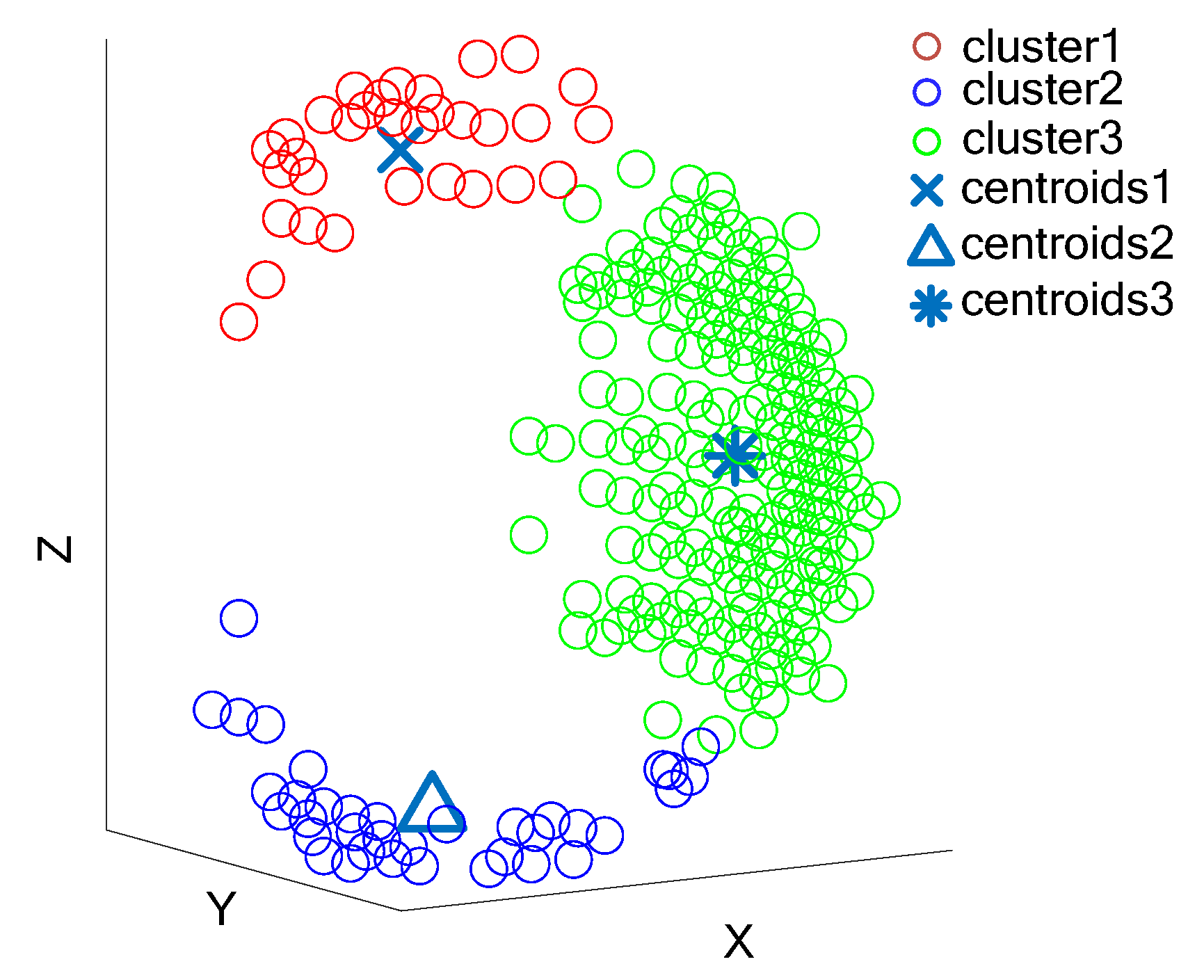
2.3. Choosing the Dexterous Workspace Center

In the following subsection, the center of the dexterous workspace for the head part is needed to estimate the end frame of the neck part. According to the structure of the snake robot in our lab, the link lengths from the first link to the sixth link for the head part are all 0.0865 m, and the length of the seventh link is 0.046 m. The workspace whose reachability index equals 100 called dexterous workspace, shown in Figure 6. We can find that it is not reasonable if we treat the centroids of the dexterous workspace as the center of the dexterous workspace. By looking at Figure 6, the dexterous workspace can be divided into three parts based on its distribution. To find a reasonable center point in the dexterous workspace, the k-means++ method is adopted [26,27]. The k-means algorithm uses a heuristic iteration process to divide the sample set into several clusters and make sure that the error sum between every sample and centroids in the same cluster has minima. Assuming that the sample set has k clusters $C_1,C_2,C_3,\dots ,C_k$, then error sum E can be calculated [26,27],

$$E=\sum _{i=1}^k\sum _{x_i\in C_i}\mathrm{d}(x_i-c_i)$$

(16)

$$c_i=\frac{1}{\mathrm{size}\left(C_i\right)}\sum _{x_i\in C_i}{x}_i$$

(17)

where $c_i$ is the centroids of the cluster $C_i$ and function $\mathrm{d}$ denotes the distance between two sample based on squared Euclidean distance. The $\mathrm{size}$ function returns the number of the samples in the cluster. k-means++ algorithm optimizes the selection of the original centroids of the clusters based on the k-means algorithm before the iteration. We choose the k-means++ algorithm to find the center of the dexterous workspace.

The k-means++ method divides the workspace into 3 clusters, and every cluster has a centroid. The results are shown in Figure 7. The centroids of the cluster 3 is chosen as the center of the dexterous workspace.

2.4. The Calculation of Joint Angles for the Neck Part

The neck part connects the base part and the head part, so the joint angles of the neck part are determined by the base part and the head part. To ensure that the head link of the head part achieves the desired pose, we need to make sure that the dexterous workspace covers the desired pose. The position of the workspace varies with the base frame of the head part in the world frame. Thus, the determination of the base frame of the head part is essential. Meanwhile, the end frame of the neck part is the base frame of the head part.

To calculate the end frame of the neck part, we denote the center of the dexterous point, the base of the head part and the end point of the base part as ${\mathit{G}}_0$, ${\mathit{B}}_0$ and ${\mathit{P}}_0$, shown in Figure 8, then

$$L_c=\parallel {\mathit{B}}_0-{\mathit{G}}_0\parallel$$

(18)

$${\mathit{r}}_d=\frac{{\mathit{G}}_0-{\mathit{P}}_0}{\parallel {\mathit{G}}_0-{\mathit{P}}_0\parallel }$$

(19)

$${\mathit{P}}_d={\mathit{G}}_0-L_c{\mathit{r}}_d$$

(20)

where ${\mathit{P}}_d$ and ${\mathit{r}}_d$ are the desired position and desired direction of the end of the neck part, respectively. Once the end frame of the neck part achieves the desired position and direction, the dexterous workspace will cover the desired pose of the head part. So next the sum $E_n$ of the error $E_p$ between the origin of the end frame of the neck part and the desired position and the error $E_d$ between the end link direction and the desire direction needs to be minimized. Suppose that the joint angles of the neck part are ${\theta }_k,{\theta }_{k+1},\dots ,{\theta }_{k+n_c-1}$, then

$${\mathit{T}}_a={}^0{\mathit{T}}_k\left({\theta }_k\right){}^k{\mathit{T}}_{k+1}\left({\theta }_{k+1}\right)\dots {}^{k+n_c-2}{\mathit{T}}_{k+n_c-1}\left({\theta }_{k+n_c-1}\right)$$

(21)

$$\begin{array}{cc}\hfill arg& \underset{q_i\in {\mathbb{R}}^n}{min}{E}_n=\parallel {\mathit{P}}_a-{\mathit{P}}_d{\parallel }_2^2+h{\parallel {\mathit{r}}_d\times {\mathit{r}}_a\parallel }_2^2\hfill \\ \hfill & s.t.q_i<=q_{lim}^{i}i=k,k+1,\dots ,k+n_c-1\hfill \end{array}$$

(22)

where ${\mathit{T}}_a$ is the transformation matrix of the frame for the end link of the neck part relative to the world frame, and ${}^0{\mathit{T}}_k$ is the transformation matrix of k-th link relative to the world frame. The neck part has $n_c$ links. ${}^{k-1}{\mathit{T}}_k$ is the transformation matrix of k-th link relative to ($k-1$)-th link for the neck part. Then ${\mathit{P}}_a$ and ${\mathit{r}}_a$ are the position and the x-axis vector of ${\mathit{T}}_a$ in the world frame. In addition, h is a coefficient. h can be set 0.01.

The illustration of the strategy is shown in Figure 8. (1) Determine the endpoint of the base part, ${\mathit{P}}_0$. ${\mathit{P}}_0$ is determined by the discretization of the backbone curve of the base part and it is used as the base point of the neck part. (2) Calculate the desired direction for the x component of the end frame of the neck part. The direction from ${\mathit{P}}_0$ to ${\mathit{G}}_0$ is used as the desired direction, which is the desired x-axis direction of the end frame for the neck part. (3) Use the center of the dexterous workspace to estimate the desired position of the origin of the end frame for the neck part. The calculation of the desired position refers to Equation (20). (4) Minimize the error $E_n$ to determine the joint angles of the neck part. The objective function and the limitation conditions of the optimization refer to Equation (22). (5) Use the TRAC-IK algorithm to solve the joint angles of the head part considering the end frame of the neck part as the base frame of the head part.

3. The Control Process of the Head

Many snake robot modules are now equipped with an inertia measure unit (IMU) for their modules [5,28,29]. An IMU usually consists of a 3-axis accelerometer and a 3-axis gyro. It is cheap and convenient to be used to estimate the posture of its carrier [30,31]. In practical applications, the purposes of the head control are often to obtain image information of the scene in front of the head camera and reach a specific position in a specific direction. Once the posture of the head of the snake robot can be estimated by the sensor information of IMU, then the restriction of the posture of the head can be reduced to the restriction of the direction of the head, which is the direction of the x-axis of the end frame for the head part. This simplification is to ensure the reliability of the strategy in the case of meeting the practical application requirements of the snake robot head control.

After the restriction is reduced, we can generate many posture frames with the same x-axis direction by rotating the one frame evenly, which are shown in Figure 9. The closest frame to the desired frame is chosen and the sensor information of the IMU is taken into account, the image corresponding frame can be modified correctly by rotating the image. The following simulations are based on this assumption.

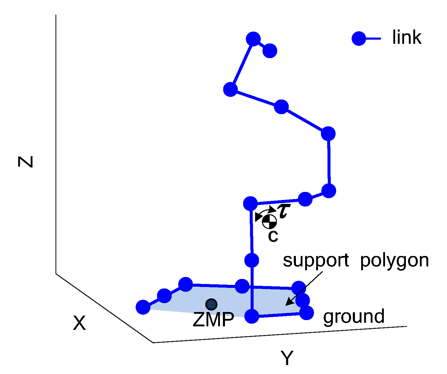
3.1. The Stability of the Motion

After the joint angles of the snake robot are obtained, the stability of the motion should be considered. In Section 2.1, the support polygon and zero-moment point are introduced. They are widely applied in the humanoid robot [32]. Moreover, Ye et al. introduced the ZMP method to the head raising of the snake robot [9] for the first time. In this section, we combine the support polygon method and the zeros-moment point method for stability analysis. Before the head of the snake robot is lifted, we need to calculate the final configuration of the snake robot body and determine whether the mass center of the body inside the support polygon. Once the center of mass is inside the support polygon, the zero-moment point method needs to be used to judge the dynamic stability of the snake robot in the movement process. For the support polygon, the equations are as follows [32],

$$\mathit{c}=\frac{{\sum }_{i=1}^N{m}_i{\mathit{P}}_i}{{\sum }_{i=1}^n{m}_i}$$

(23)

$$\mathit{C}=\mathrm{polygon}({\mathit{p}}_0,{\mathit{p}}_1,\dots ,{\mathit{p}}_{k-1})$$

(24)

where $m_i$ indicates the mass of the i-th link of the snake robot and ${\mathit{P}}_i$ represents the center of mass of i-th link. N denotes the number of links of the robot. $\mathit{c}$ is the center of the mass of the snake robot. ${\mathit{p}}_i$ is the endpoint of the link for the base part. The function $\mathrm{polygon}$ outputs a polygon constructed by the input points. The robot is statically stable if $\mathit{c}\in \mathit{C}$.

For the process of the motion for the robot, the ZMP method is used for dynamically stability for the snake robot. Since the ZMP method is based on the torque equilibrium, the linear velocity and the angular velocity of the link should be calculated first. Assuming that the linear velocity and angular velocity of the i-th link are known [32], then

$${}^0{\mathit{v}}_j={}^0{\mathit{v}}_i+{}^0{\mathit{\omega }}_i\times {}^0{\mathit{R}}_i{}^i{\mathit{b}}_j$$

(25)

$${}^0{\mathit{\omega }}_j={}^0{\mathit{\omega }}_i+{}^0{\mathit{R}}_i\times {}^i{\mathit{z}}_j{\dot{q}}_j$$

(26)

where ${}^0{\mathit{v}}_j$ and ${}^0{\mathit{\omega }}_j$ are the linear velocity and angular velocity of the j-th link represented in the world frame, frame 0. The ${}^i{\mathit{z}}_j$ is the z-axis of frame j represented in frame i. ${}^0{\mathit{R}}_i$ is the rotation matrix of the frame i relative to the frame 0. ${}^i{\mathit{b}}_j$ is the joint position vector for j-th link represented in the i-th frame. ${\dot{q}}_j$ is the derivative of j-th joint angle relative to time.

Next the velocities of the links are used to calculate the linear momentum and angular momentum of the robot [32],

$${}^0\dot{{\mathit{c}}_j}={}^0{\mathit{v}}_j+{}^0{\mathit{\omega }}_j\times \left({}^0{\mathit{R}}_j{\overline{\mathit{c}}}_j\right)$$

(27)

$${}^0{\mathcal{P}}_j=m_j{}^0{\dot{\mathit{c}}}_j$$

(28)

$${}^0\mathcal{P}=\sum _{j=1}^N{}^0{\mathcal{P}}_j$$

(29)

$${}^0{\mathcal{L}}_j={}^0{\mathit{c}}_j\times {}^0{\mathcal{P}}_j+{}^0{\mathit{R}}_j{\overline{\mathit{I}}}_j{}^0{\mathit{R}}_j^{\mathrm{T}}{}^0{\mathit{\omega }}_j$$

(30)

$${}^0\mathcal{L}=\sum _{j=1}^N{}^0{\mathcal{L}}_j$$

(31)

where ${\overline{c}}_j$ indicates the coordinate of the center of mass for the j-th link represented in frame j. In addition, ${}^0{\dot{\mathit{c}}}_j$ denotes the derivative of the center of mass of the j-th respect to time represented in the world frame. ${}^0{\mathcal{P}}_j$ and ${}^0\mathcal{P}$ represent the linear momentum for i-th link and the robot respectively. ${}^0{\mathcal{L}}_j$ and ${}^0\mathcal{L}$ represent the angular momentum for i-th link and the robot respectively. ${\overline{\mathit{I}}}_j$ is the inertia tensor matrix of the j-th link relative to the local frame.

Then the ZMP can be solved based on the dynamics algorithm [32],

$$\mathit{\tau }=\mathit{p}\times \mathit{f}+{\mathit{\tau }}_p$$

(32)

$${}^0\dot{\mathcal{P}}=M\mathit{g}+\mathit{f}$$

(33)

$${}^0\dot{\mathcal{L}}=\mathit{c}\times M\mathit{g}+\mathit{\tau }$$

(34)

substitute (33) and (34) into (32), we have

$${\mathit{\tau }}_p={}^0\dot{\mathcal{L}}-\mathit{c}\times M\mathit{g}+({}^0\dot{\mathcal{P}}-M\mathit{g})\times \mathit{p}$$

(35)

where $\mathit{f}$ is the reaction force of the ground to the link. In addition, $\mathit{p}$ denotes the zero-moment point, $M={\sum }_{j=1}^N{m}_j$. $\mathit{g}$ is the gravity acceleration vector. Thus, we can obtain [32],

$${\tau }_{px}={\dot{\mathcal{L}}}_x+Mgy+{\dot{\mathcal{P}}}_y{p}_z-({\dot{\mathcal{P}}}_z+Mg)p_y$$

(36)

$${\tau }_{py}={\dot{\mathcal{L}}}_y-Mgx-{\dot{\mathcal{P}}}_x{p}_z+({\dot{\mathcal{P}}}_z+Mg)p_x$$

(37)

where

$$\left\{\begin{array}{c}{}^0\mathcal{P}={\left[{\mathcal{P}}_x{\mathcal{P}}_y{\mathcal{P}}_z\right]}^{\mathrm{T}}\hfill \\ {}^0\mathcal{L}={\left[{\mathcal{L}}_x{\mathcal{L}}_y{\mathcal{L}}_z\right]}^{\mathrm{T}}\hfill \\ \mathit{c}={\left[xyz\right]}^{\mathrm{T}}\hfill \\ \mathit{g}={[00-g]}^{\mathrm{T}}\hfill \\ \mathit{p}={\left[p_x{p}_y{p}_z\right]}^{\mathrm{T}}\hfill \end{array}\right.$$

(38)

Let the x component ${\tau }_{px}$ and y component ${\tau }_{py}$ of the moment ${\mathit{\tau }}_p$ be 0. The $p_x$ and $p_y$ of the ZMP can be solved [32].

$$p_x=\frac{Mgx+p_z{\dot{\mathcal{P}}}_x-{\dot{\mathcal{L}}}_y}{Mg+{\dot{\mathcal{P}}}_z}$$

(39)

$$p_y=\frac{Mgy+p_z{\dot{\mathcal{P}}}_y+{\dot{\mathcal{L}}}_x}{Mg+{\dot{\mathcal{P}}}_z}$$

(40)

Then we have $p_z=0$ considering that the snake robot locomotes on the ground. If the projection of the ZMP on the ground, $(p_x,p_y)$ lies inside the support polygon, the snake robot is dynamically stable. The illustration is shown in Figure 10.

3.2. The Trajectory Planning of the Overall Body in Cartesian Space

After the joint positions of the robot are solved, A multi-segment trajectories interpolation method [17] for joint angles of the robot is adopted. However, the head of the snake robot sometimes will hit the ground and lose the balance of the body. The specific situation is shown in Figure 11. The initial state of the snake robot is like State 1, and then the body of the snake robot moves to State 2. The head of the robot will hit the ground since only the interpolations of the joint angles are considered.

To solve the above problem, an interpolation method of the overall body of the snake robot based on the Cartesian space is proposed. The joint positions of the neck part and head part in the Cartesian space for the initial configuration are assumed ${\mathit{p}}_{s0}$, ${\mathit{p}}_{s1}$, ..., ${\mathit{p}}_{sn-1}$, and ones for the final configuration are assumed ${\mathit{p}}_{f0}$, ${\mathit{p}}_{f1}$, ..., ${\mathit{p}}_{fn-1}$. First, ${\mathit{p}}_{si}$ and ${\mathit{p}}_{fi}$ is linear interpolated. However, the other interpolation methods, such as quadratic interpolation and cubic interpolation, can also be adopted. For simplifying the calculation, the linear interpolation is adopted. Then we have

$$\begin{array}{cc}\hfill {\mathit{p}}_{ij}& ={\mathit{p}}_{fi}+(1-t_j){\mathit{p}}_{si},i=0,1,2,\dots ,n-1j=0,1,\hfill \\ \hfill & 2,\dots ,m0\le t_0\le t_1\le \dots \le t_j\le \dots \le t_m\le 1\hfill \end{array}$$

(41)

where ${\mathit{p}}_{ij}$ represents the interpolation position of i-th joint corresponding parameter $t_j$. In addition, every $t_j$ can be used to interpolate a configuration of the snake robot.

Assuming the transformation matrix of the starting frame of the neck part is ${\mathit{T}}_0$ and the D-H frames {$x_i,y_i,z_i$} are constructed as shown in Figure 12, the links of the neck part and head part approach the line segments generated by the linear interpolation. Then we have

$${\theta }_i=\pi /2-arccos({\mathit{T}}_y·\frac{{\mathit{l}}_{\mathrm{proj}}^i}{\parallel {\mathit{l}}_{\mathrm{proj}}^i\parallel })i=0,1,2,\dots ,n-1$$

(42)

$${\mathit{l}}_{\mathrm{proj}}^i={\mathit{l}}_i-({\mathit{l}}_i·{\mathit{T}}_z){\mathit{T}}_{z}i=0,1,2,\dots ,n-1$$

(43)

$${\mathit{l}}_i=\frac{{\mathit{p}}_{i+1j}-{\mathit{p}}_{ij}}{\parallel {\mathit{p}}_{i+1j}-{\mathit{p}}_{ij}\parallel }i=0,1,2,\dots ,n-1$$

(44)

where ${\theta }_i$ denotes the i-th joint angles from the neck part, and ${\mathit{T}}_i$ indicates the transformation matrix of the i-th joint frame relative to the world frame. ${\mathit{T}}_y$ and ${\mathit{T}}_z$ are the y-axis vector and z-axis vector of the local frame of ${\mathit{T}}_i$ for i-th joint. ”·” is the dot product operator. $\arccos$ is represents the inverse trigonometric function of cosine. The interpolation result of the proposed method is shown in Figure 13.

3.3. The Process of the Control

When the joint angles of snake robot can be determined, we conclude the control process as follows.

(1)

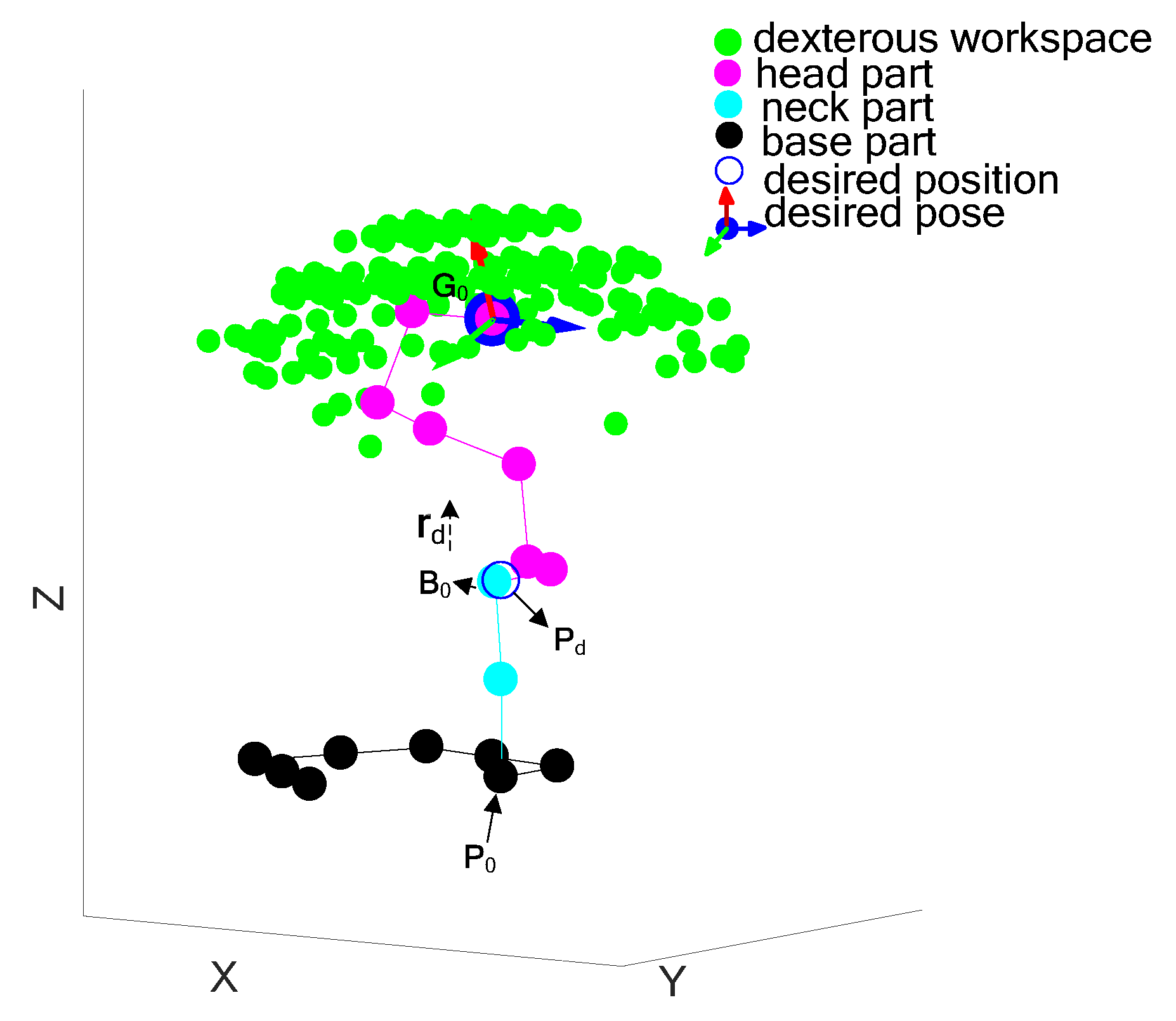
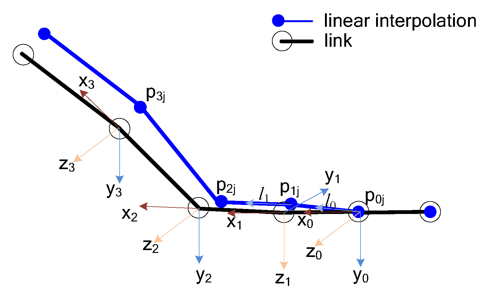
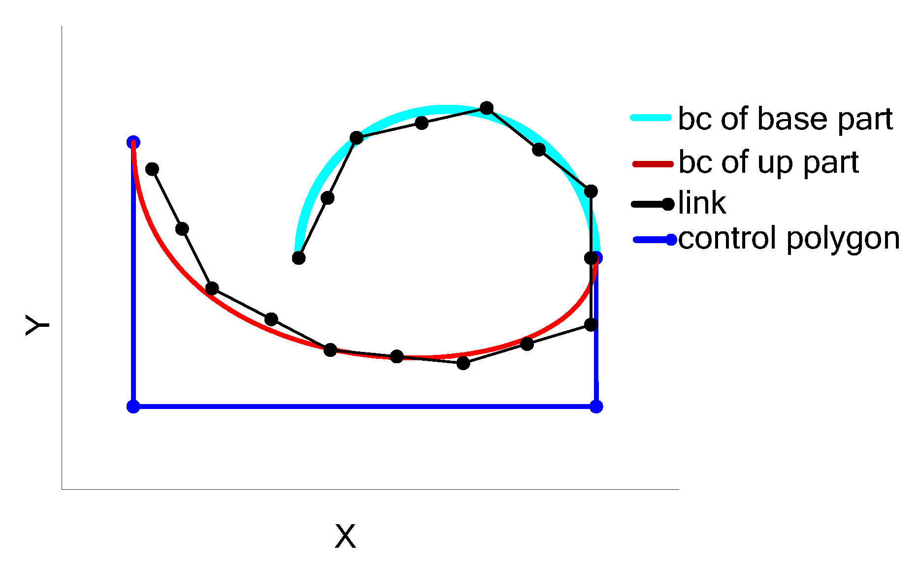
Discretize the backbone curve of the snake robot to obtain the initial configuration of the snake robot, and the backbone curve and the links are shown in Figure 14. The backbone curve of the base part is a plane arc and the backbone curve of the neck part and head part is a plane cubic Bezier curve with four control point. The two backbone curves are connected smoothly.

(2)

Plan the current configuration to the initial configuration for the snake robot.

(3)

Determine the desired position and direction for the end link of the neck part using the desired pose of the head link and the dexterous workspace of the head part, and judge whether the desired position is in an accepted range, which satisfies ${\sum }_{i=k}^{k+n_c-1}{L}_i-\parallel {\mathit{P}}_{hd}-{\mathit{P}}_0\parallel -L_c<L_0$ and ${\sum }_{i=k}^{k+n_c-1}{L}_i>\parallel {\mathit{P}}_{hd}-{\mathit{P}}_0\parallel -L_c$. ${\mathit{P}}_{hd}$ indicates the desired position of the head link of the head part. If the conditions are not satisfied, use the rolling gait or turn in place [33] to adjust the location and orientation of the overall body in the world frame.

(4)

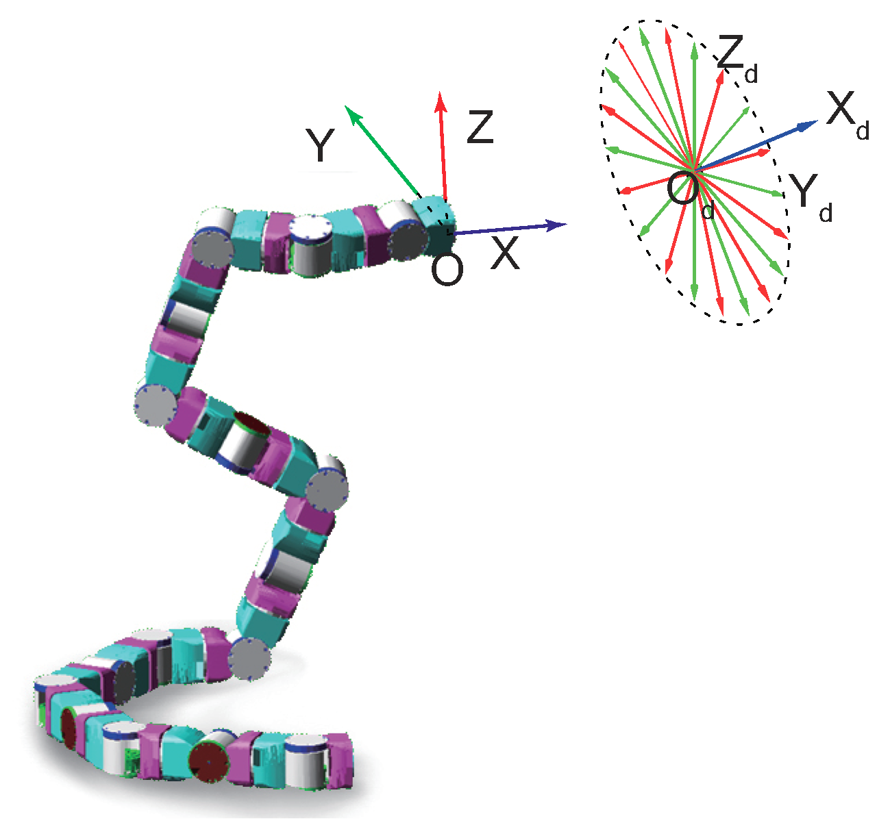
By rotating a frame evenly, many desired pose frames with the same x-axis direction as the desired direction are created. In addition, the solution we need is selected among solutions of these pose frames.

(5)

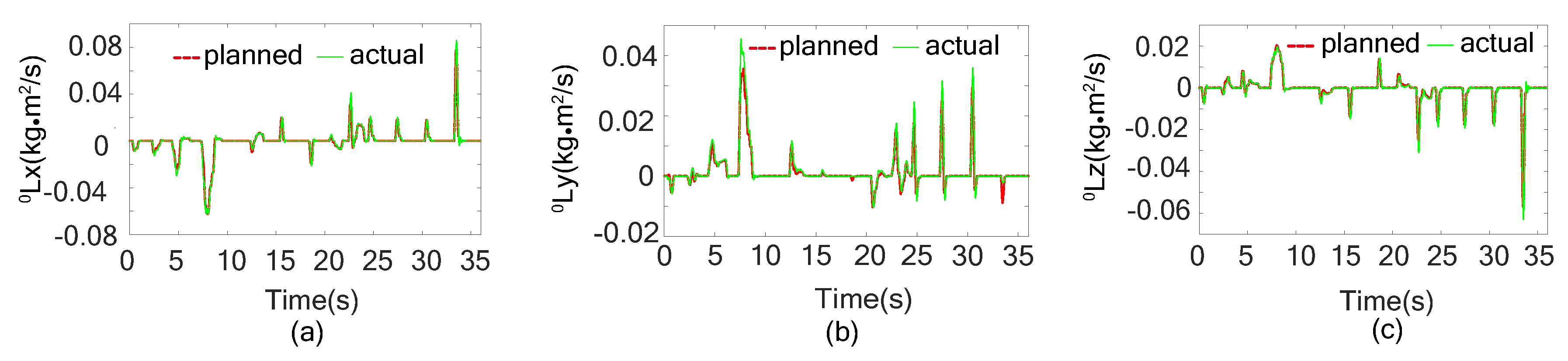
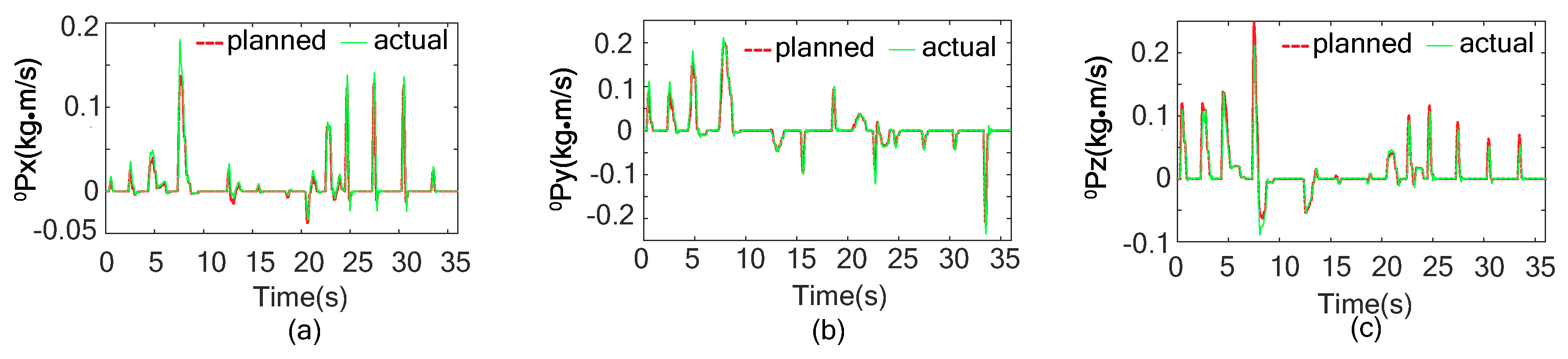
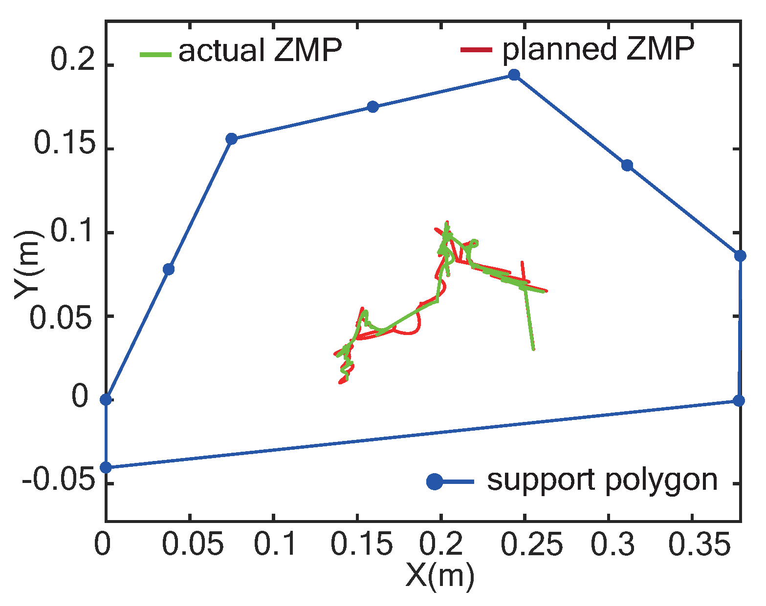
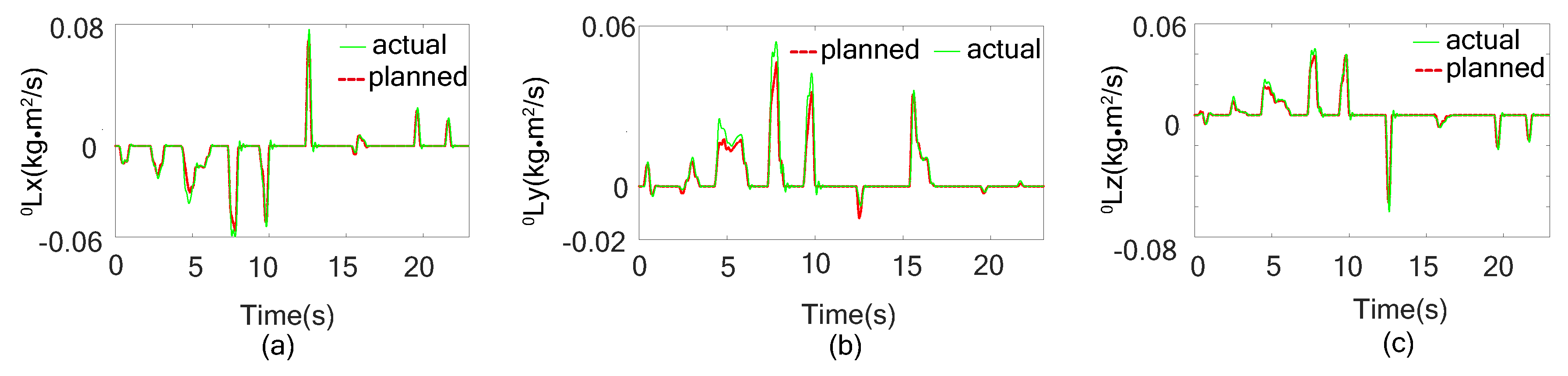
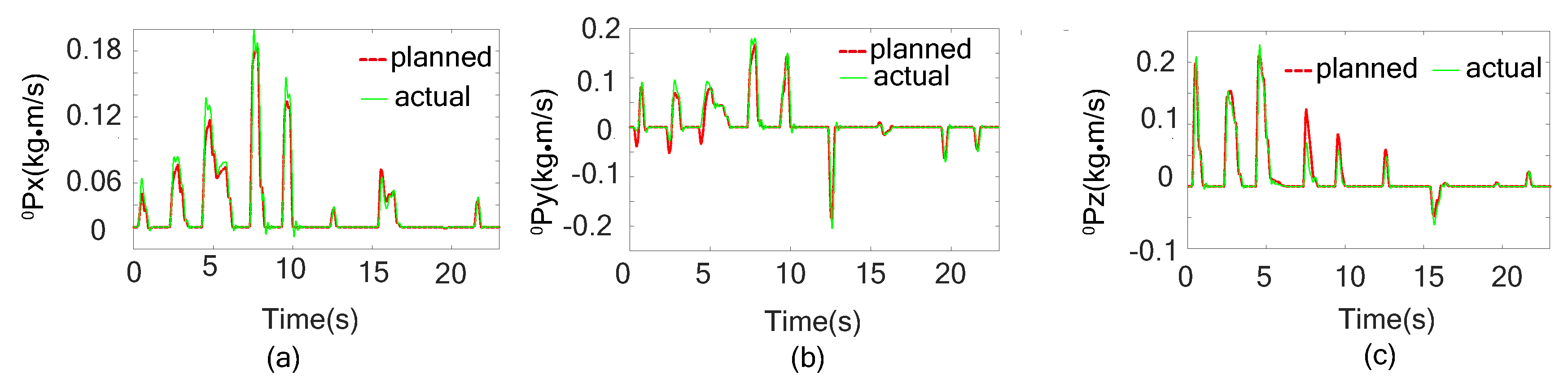
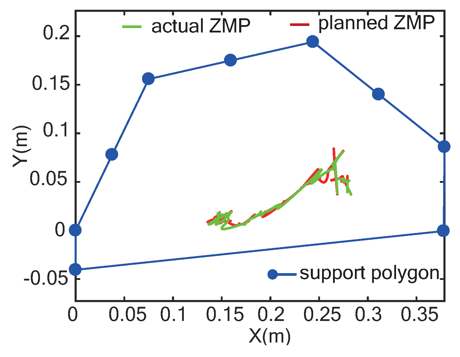
Plan the trajectory of the snake robot to the final configuration, then use the support polygon method and the ZMP method to assert the static stability and dynamical stability of the motion. Select a stable trajectory.

(6)

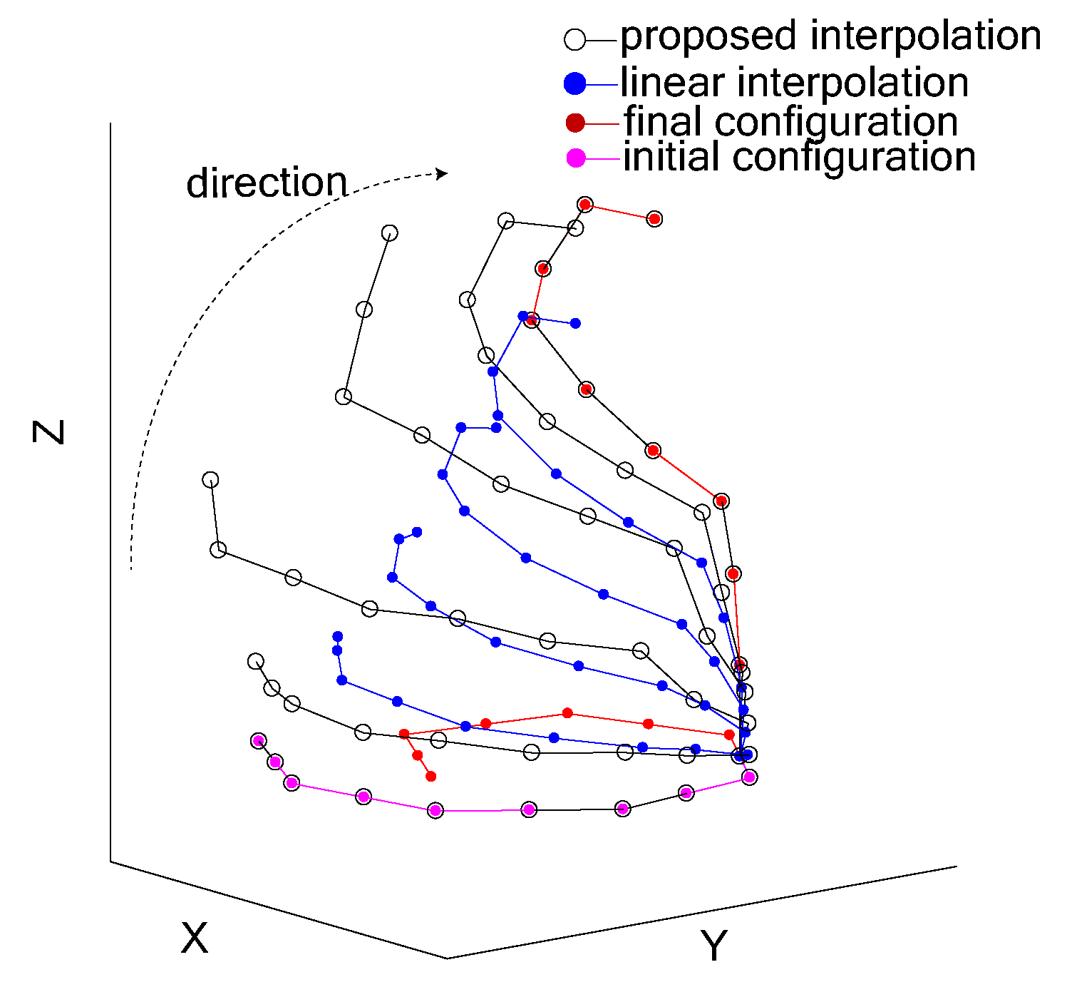
Use the proposed trajectory planning method of the overall body in Cartesian space to avoid collision of the snake robot with the ground.

These six steps can ensure the head of the snake robot achieve the desired position and desired direction.

4. Simulations of the Head Control

To verify the effectiveness of the head control strategy, the simulations that the head of the snake robot catches the desired virtual spheres and gets through a hole on a wall are conducted. These simulations are completed by the joint work of MATLAB and dynamics software. The trajectory planning in the joint space is completed in the Simulink of the MATLAB and the Simulink is taken as a central controller. In addition, a PD with a gravity compensation controller is adopted to ensure the precision of the trajectory tracking. The snake robot consists of 16 modules. In addition, there are 8 links, 2 links and 7 links for the base part, neck part and head part, respectively. The architecture of the snake robot is shown in Figure 15. The base part, neck part and head part are shown in Figure 1b. The specific parameters of the snake robot are shown in

Table 3. The overview of the snake robot.

dimensions	module: 4.3 cm × 4.3 cm × 8.65 cm
	length (full 16 module robot): 138.4 cm
	length (start link): 4.05 cm
	length (head link): 4.6 cm
mass	module: 0.2 kg
	full 16 module robot: 3.2 kg
joint limit	±90 degree

. The working computer for the simulation has 2.50 GHz Intel Core i7 CPU and 8 GB RAM. For our snake robot with 17 links, the solving time consists of the calculating time of the TRAC-IK solver and the computation time of the optimization algorithm. The instantaneous ZMP is calculated with the snake robot moving. The total solving process can be completed in 100 ms while we need to calculate 10 times for a specific direction of the snake robot head in simulations. Thus, it can meet the requirement of the real-time of robot control since the joint controller can also interpolate the joint angles with a shorter control period to control the motion of joints. The control period of the joint controller is 2 ms. Moreover, the positions of the spheres and hole are known in advance and the pose of the base frame of the neck part is obtained in time in the simulation process.

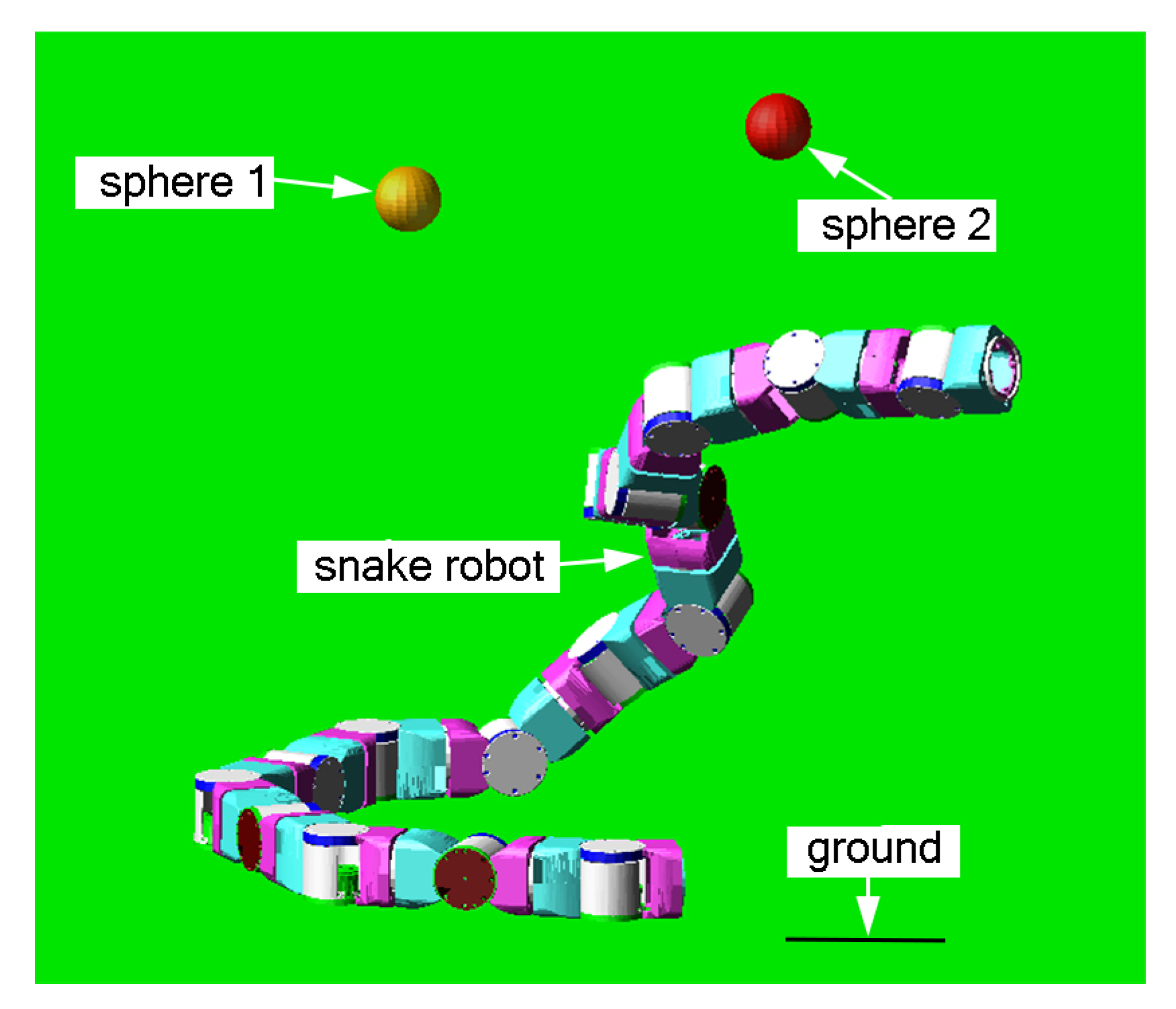
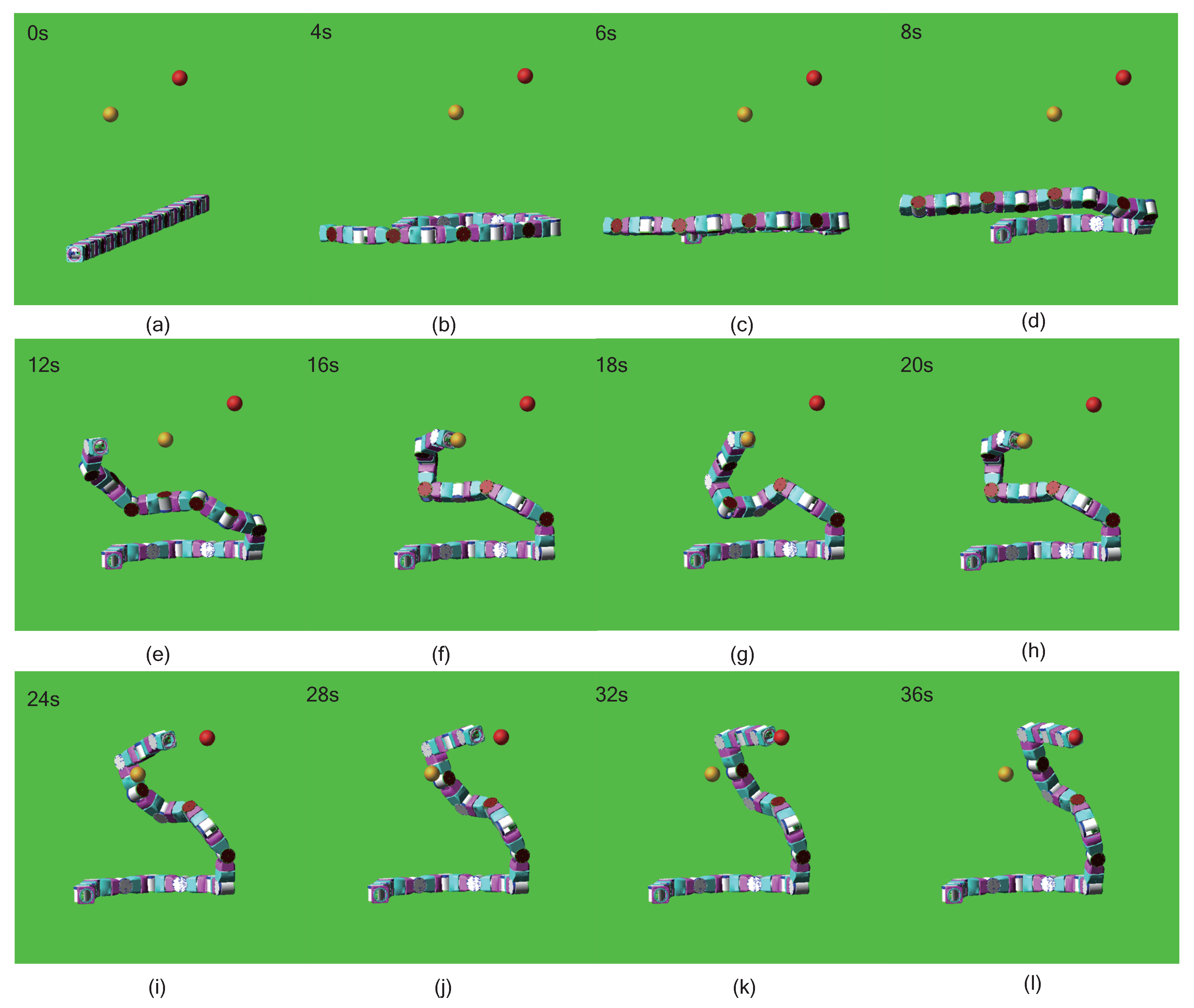
4.1. The Simulation of Catching the Virtual Spheres

The platform of simulation is shown in Figure 16. The diameters of the two spheres are both 4 cm. The coordinate of the center of the mass for the sphere 1 is (−4.05 × ${10}^{-2}$, 0.5443, 0.3) m, and that of sphere 2 is (0.1505, 0.5076, 0.3954) m. The simulation of the snake robot needs to complete the task that the head of the robot moves to catch the sphere 1 from the current state and then transforms to catch the sphere 2. The process of the simulation is shown in Figure 17. The total time of the simulation is 36 s. The current state of the snake robot is shown in Figure 17a. To ensure the stability of the motion, the snake robot transforms to the initial state from the current state as in Figure 17b. To get the reliable solution of the inverse kinematics, two spheres must be in the accepted range using the item (3) in Section 3.3, otherwise the location of the snake robot needs to be adjusted. The controller can obtain the information of the pose of the base frame for the neck part in the process. Then the joint angles of the neck part and head part for achieving the sphere 1 are solved using the proposed strategy. Then, the proposed trajectory planning method of the overall body in Cartesian space is used to plan the initial state to the state of catching sphere 1. The stability of the motion is determined by the support polygon and ZMP methods. The process for catching sphere 1 is illustrated in Figure 17c–g. After that, the joint angles of the neck part and head part for catching the sphere 2 are solved using the proposed strategy. Then the trajectories of the joints from the state catching sphere 1 to state catching sphere 2 are planned by the proposed method. The process is shown in Figure 17h–l. The position error between the head link frame and the sphere is 1.8mm and the direction error between the x-axis of the head link frame and the desired direction is 0.76 degrees. The angular and linear momentum of the snake robot for the planned trajectory and the actual dynamics simulation in the world frame are shown in Figure 18 and Figure 19. The maximum errors of the angular and linear momentum magnitudes of the planned trajectory and the simulation are 0.0383 kg·m${}^2$/s and 0.216 kg·m/s. The projections of ZMPs of the snake robot for the planned trajectory and the actual dynamics simulation on the ground are shown in Figure 20. Since they are both inside the support polygon, the motion is stable.

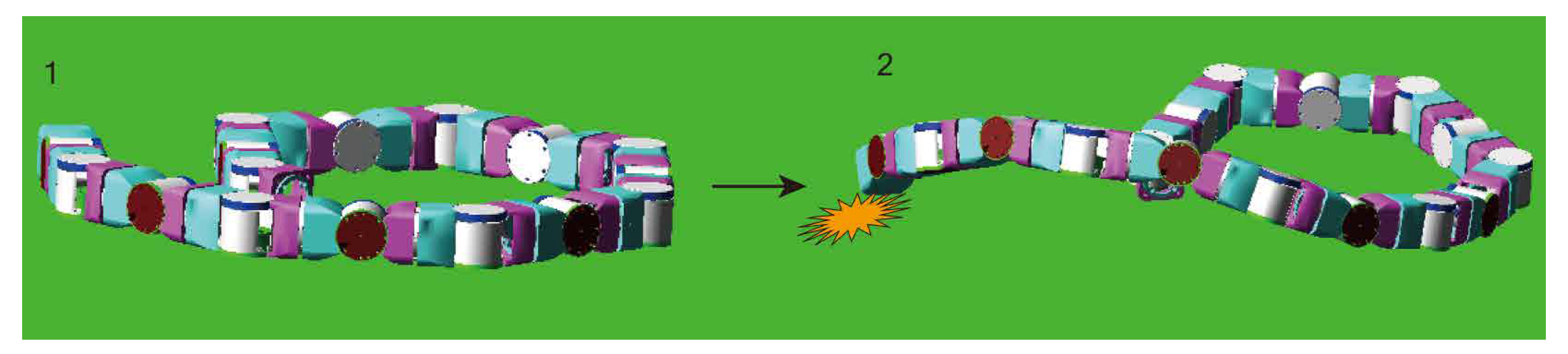
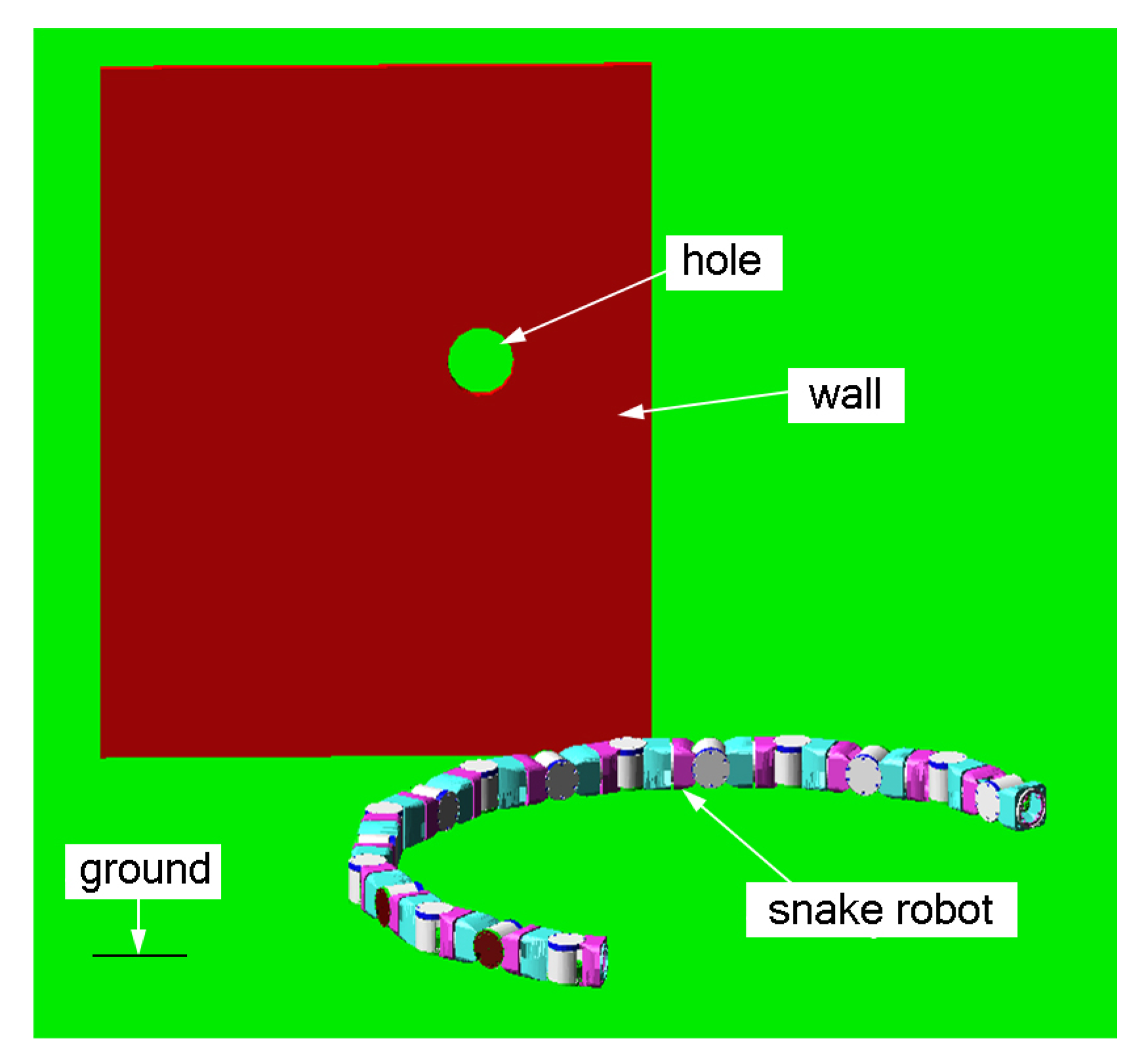
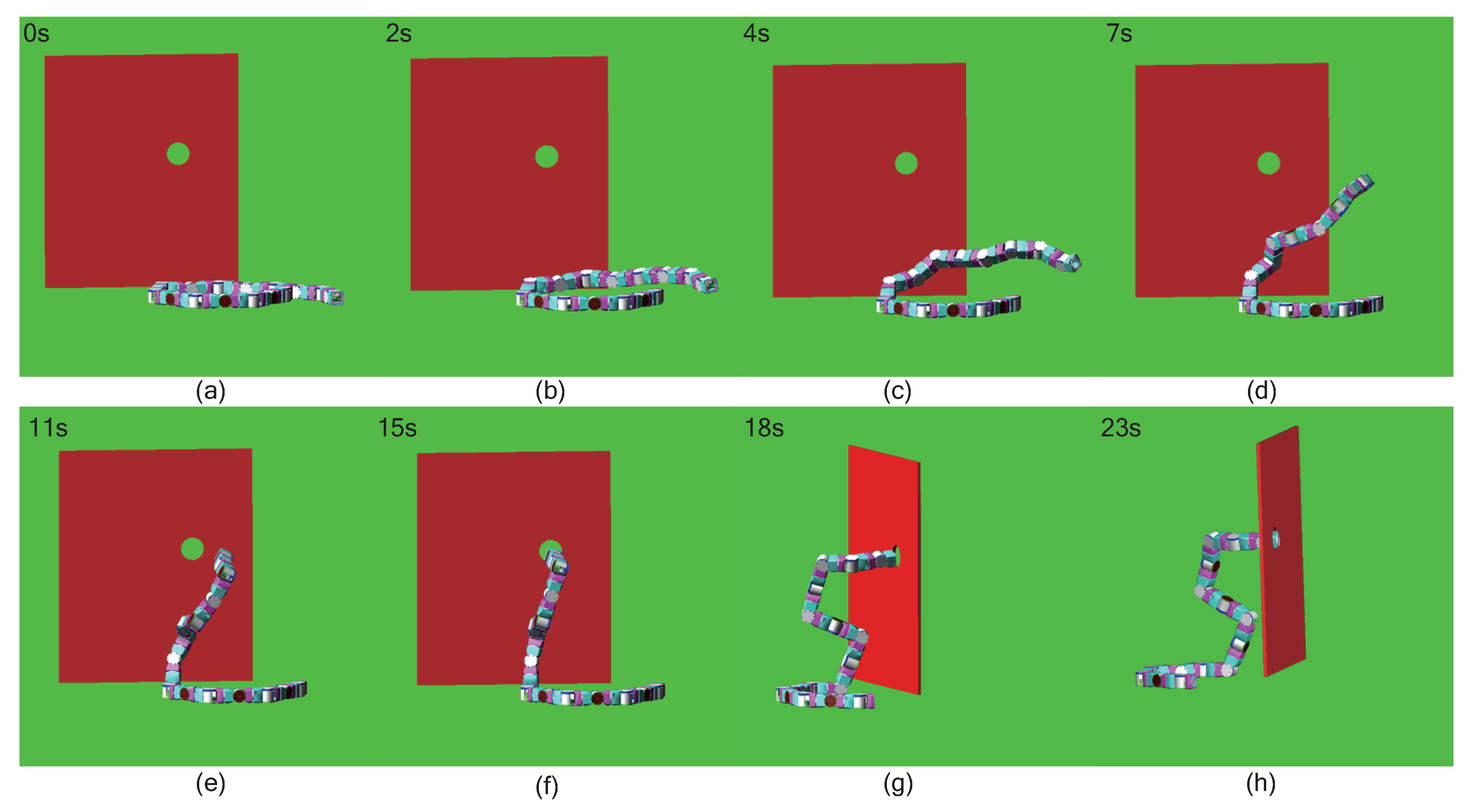
4.2. The Simulation of Getting through a Hole

The simulation scenario for getting through a hole is shown in Figure 21. The diameter of the hole is 7 cm. The dimension of the wall is 0.7 m × 0.58 m × 0.01 m. The coordinate of the hole is (0.2, 0.5, 0.4) m. The process of the snake robot getting through a hole on the wall is shown in Figure 22. The total time of the process is 23 s. To ensure that the center of the mass of the snake robot is inside the support polygon of the base part before the head raising, the snake robot is transformed to the initial state shown in Figure 22a. First, the hole is guaranteed in the accepted range using the item (3) in Section 3.3. Then the joint angles for the pose with a desired direction paralleling to the axis of the cylinder hole and position close to the hole shown in Figure 22f is solved. The proposed trajectory planning method in Cartesian space is used to plan the state shown in Figure 22a to the state shown in Figure 22f. The planning generates the intermediate states as in Figure 22b–e. A multi-segment trajectories interpolation method is adopted to interpolate the joint angles among these states. Then the ZMP method is used to determine whether the motion of the robot is stable, and the parameter of the multi-segment trajectories interpolation method is tuned if not. Then two poses with a desired direction paralleling to the axis of the cylinder hole and a position closer to the hole shown in Figure 22g,h are solved. The joint angles with the smallest change compared to the joint angle solution of the previous state will be preserved. Then finally, the head link of the snake robot got through the hole on the wall in Figure 22i. The position error between the head link frame and the hole is 1.39 mm and the direction error between the x-axis of the head link frame and the desired direction is 0.95 degree. The angular and linear momentum of the snake robot for the planned trajectory and the actual dynamics simulation are shown in Figure 23 and Figure 24. The maximum errors of the angular and linear momentum magnitudes of the planned trajectory and the simulation are 0.0416 kg·m${}^2$/s and 0.195 kg·m/s. The projections of ZMPs of the snake robot for the planned trajectory and the actual dynamics simulation on the ground are shown in Figure 25. Since they are both inside the support polygon, the motion is stable.

5. Discussion and Conclusions

A head control strategy for the snake robot based on segmented kinematics is proposed in this article. Through segmented control of the base part, the neck part and the head part of the snake robot, the accurate control of the head of the snake robot is achieved. To enhance the stability of the snake robot when the head is lifted, the parameters of the backbone curve of the base part are optimized. The existing inverse kinematics algorithms are used in the snake robot and the solve rate of these algorithms are compared. Then TRAC-IK algorithm is selected. In addition, the dexterous workspaces of the 6 DOFs and 7 DOFs solved by the TRAC-IK algorithm are compared to determine the number of the links for the head part. The neck part is determined by the dexterous workspace of the head part and the desired pose of the head link. After the base part and the neck part is solved, the end link of the neck part is treated as the base of the head part. Then joint angles of the head part are solved using the TRAC-IK algorithm. The trajectory planning method of the overall body in Cartesian space is proposed to avoid the collision between the body and the ground. To ensure the motion stability of the head, the support polygon method and ZMP method are adopted. Eventually, the dynamic simulations of the head of the snake robot catching spheres and getting through the hole on the wall validate the effectiveness of the control strategy.

However, some problems are needed to solve in the future. First, we will spend time studying how to add some visual sensors on the snake robot head and then apply the strategy to the actual acquisition and processing of the snake robot camera image. Moreover, the experimental validation will be conducted in the next stage of the research. After that, some parameters of the simulation model need to be improved to adapt to the real snake robot body, especially the dynamical parameters. To get the accurate dynamic parameters of the snake robot is hard work, but it is very important for the calculation of ZMP according to Section 3.1. Moreover, some optimal trajectories for the head control need to be selected for the snake robot since the motors of the snake robot usually only output relatively small torque. For energy-saving and good mobility, the module of the snake robot is designed to be smaller, which limits the output torque of the motor. Thus, we will conduct the work of selecting the trajectory with the affordable torque requirements for our snake robot in the future.

References

1. Sanfilippo, F.; Azpiazu, J.; Marafioti, G.; Transeth, A.A.; Stavdahl, Ø.; Liljebäck, P. Perception-driven obstacle-aided locomotion for snake robots: the state of the art, challenges and possibilities. Appl. Sci. 2017, 7, 336. [Google Scholar] [CrossRef]
2. Wang, K.; Gao, W.; Ma, S. Snake-like robot with fusion gait for high environmental adaptability: Design, modeling, and experiment. Appl. Sci. 2017, 7, 1133. [Google Scholar] [CrossRef]
3. Kelasidi, E.; Jesmani, M.; Pettersen, K.; Gravdahl, J. Locomotion efficiency optimization of biologically inspired snake robots. Appl. Sci. 2018, 8, 80. [Google Scholar] [CrossRef]
4. Mu, Z.; Wang, H.; Xu, W.; Liu, T.; Wang, H. Two types of snake-like robots for complex environment exploration: Design, development, and experiment. Adv. Mech. Eng. 2017, 9, 1–15. [Google Scholar] [CrossRef]
5. Rollinson, D.; Bilgen, Y.; Brown, B.; Enner, F.; Ford, S.; Layton, C.; Rembisz, J.; Schwerin, M.; Willig, A.; Velagapudi, P. Design and architecture of a series elastic snake robot. In Proceedings of the IEEE/RSJ International Conference on Intelligent Robots & Systems, Chicago, IL, USA, 14–18 September 2014. [Google Scholar]
6. Sanfilippo, F.; Stavdahl, Ø.; Liljebäck, P. SnakeSIM: A ROS-based control and simulation framework for perception-driven obstacle-aided locomotion of snake robots. Artif. Life Robot. 2018, 23, 449–458. [Google Scholar] [CrossRef]
7. Ariizumi, R.; Tanaka, M.; Matsuno, F. Analysis and heading control of continuum planar snake robot based on kinematics and a general solution thereof. Adv. Robot. 2016, 30, 301–314. [Google Scholar] [CrossRef]
8. Tanaka, M.; Matsuno, F. Modeling and control of head raising snake robots by using kinematic redundancy. J. Intell. Robot. Syst. 2014, 75, 53–69. [Google Scholar] [CrossRef]
9. Ye, C.; Ma, S.; Li, B.; Wang, Y. Head-raising motion of snake-like robots. In Proceedings of the 2004 IEEE International Conference on Robotics and Biomimetics, Shenyang, China, 22–26 August 2004; pp. 595–600. [Google Scholar]
10. Zhang, X.; Liu, J.; Ju, Z.; Yang, C. Head-raising of snake robots based on a predefined spiral curve method. Appl. Sci. 2018, 8, 2011. [Google Scholar] [CrossRef]
11. Chirikjian, G.S.; Burdick, J.W. A modal approach to hyper-redundant manipulator kinematics. IEEE Trans. Robot. Autom. 1994, 10, 343–354. [Google Scholar] [CrossRef]
12. Zhen, W.; Gong, C.; Choset, H. Modeling rolling gaits of a snake robot. In Proceedings of the 2015 IEEE International Conference on Robotics and Automation (ICRA), Seattle, WA, USA, 26–30 May 2015; pp. 3741–3746. [Google Scholar]
13. Kamegawa, T.; Harada, T.; Gofuku, A. Realization of cylinder climbing locomotion with helical form by a snake robot with passive wheels. In Proceedings of the 2009 IEEE International Conference on Robotics and Automation, Kobe, Japan, 12–17 May 2009; pp. 3067–3072. [Google Scholar]
14. Zacharias, F.; Borst, C.; Hirzinger, G. Capturing robot workspace structure: Representing robot capabilities. In Proceedings of the IEEE/RSJ International Conference on Intelligent Robots & Systems, San Diego, CA, USA, 29 October–2 November 2007. [Google Scholar]
15. Smits, R. KDL: Kinematics and Dynamics Library. 2019. Available online: http://wiki.ros.org/orocos_kdl (accessed on 16 November 2019).
16. Siciliano, B.; Sciavicco, L.; Villani, L.; Oriolo, G. Robotics: Modelling, Planning and Control; Springer Science & Business Media: Berlin, Germany, 2010. [Google Scholar]
17. Corke, P.I. Robotics, Vision & Control: Fundamental Algorithms in MATLAB, 2nd ed.; Springer: Berlin, Germany, 2017; ISBN 978-3-319-54413-7. [Google Scholar]
18. Beeson, P.; Ames, B. TRAC-IK: An Open-Source Library for Improved Solving of Generic Inverse Kinematics. In Proceedings of the 2015 IEEE-RAS 15th International Conference on Humanoid Robots (Humanoids), Seoul, Korea, 3–5 November 2015. [Google Scholar]
19. Bing, Z.; Cheng, L.; Chen, G.; RaHrbein, F.; Huang, K.; Knoll, A. Towards autonomous locomotion: CPG-based control of smooth 3D slithering gait transition of a snake-like robot. Bioinspir. Biomim. 2017, 12, 035001. [Google Scholar] [CrossRef] [PubMed]
20. Melo, K. Modular snake robot velocity for side-winding gaits. In Proceedings of the 2015 IEEE International Conference on Robotics and Automation (ICRA), Seattle, WA, USA, 26–30 May 2015; pp. 3716–3722. [Google Scholar]
21. Kajita, S.; Hirukawa, H.; Harada, K.; Yokoi, K. Introduction to Humanoid Robotics; Springer: Berlin, Germany, 2014; Volume 101. [Google Scholar]
22. Yamada, H.; Hirose, S. Approximations to continuous curves of Active Cord Mechanism made of arc-shaped joints or double joints. In Proceedings of the IEEE International Conference on Robotics & Automation, Anchorage, AK, USA, 3–7 May 2010. [Google Scholar]
23. Oprea, J. Differential Geometry and Its Applications; American Mathematical Soc.: Providence, RI, USA, 2019; Volume 59. [Google Scholar]
24. Yoshikawa, T. Basic optimization methods of redundant manipulators. Lab. Robot. Autom. 1996, 8, 49–60. [Google Scholar] [CrossRef]
25. Nocedal, J.; Wright, S.J. Numerical Optimization, 2nd ed.; Springer: New York, NY, USA, 2006. [Google Scholar]
26. Spath, H. Cluster Dissection and Analysis: Theory, FORTRAN Programs, Examples; Horwood: Bristol, UK, 1985. [Google Scholar]
27. Arthur, D.; Vassilvitskii, S. k-means++: The advantages of careful seeding. In Proceedings of the Eighteenth Annual ACM-SIAM Symposium on Discrete Algorithms, Society for Industrial and Applied Mathematics, Philadelphia, PA, USA, 7–9 January 2007; pp. 1027–1035. [Google Scholar]
28. Bing, Z.; Long, C.; Zhong, A.; Zhang, F.; Kai, H.; Knoll, A. Slope angle estimation based on multi-sensor fusion for a snake-like robot. In Proceedings of the International Conference on Information Fusion, Xi’an, China, 10–13 July 2017. [Google Scholar]
29. Bando, Y.; Suhara, H.; Tanaka, M.; Kamegawa, T.; Itoyama, K.; Yoshii, K.; Matsuno, F.; Okuno, H.G. Sound-based online localization for an in-pipe snake robot. In Proceedings of the IEEE International Symposium on Safety, Lausanne, Switzerland, 23–27 October 2016. [Google Scholar]
30. Euston, M.; Coote, P.; Mahony, R.; Kim, J.; Hamel, T. A Complementary Filter for Attitude Estimation of a Fixed-Wing UAV. In Proceedings of the IEEE/RSJ International Conference on Intelligent Robots & Systems, Nice, France, 22–26 September 2008. [Google Scholar]
31. Madgwick, S. An efficient orientation filter for inertial and inertial/magnetic sensor arrays. Rep. x-io Univ. Bristol UK 2010, 25, 113–118. [Google Scholar]
32. Dekker, M. Zero-Moment Point Method for Stable Biped Walking; Eindhoven University of Technology: Eindhoven, The Netherlands, 2009. [Google Scholar]
33. Xiao, X.; Cappo, E.; Zhen, W.; Dai, J.; Sun, K.; Gong, C.; Travers, M.J.; Choset, H. Locomotive reduction for snake robots. In Proceedings of the 2015 IEEE International Conference on Robotics and Automation (ICRA), Seattle, WA, USA, 26–30 May 2015; pp. 3735–3740. [Google Scholar]
Figure 1. (a) The axis of each joint is rotated 90 degree relative to the previous joint axis; yaw joint generates rotation out of the plane, while pitch joint generates rotation in the plane in this illustration. (b) The overview of the snake robot.
Applsci 09 05104 g001
Figure 2. The support polygon constructed by the base part of the snake robot and the plane arc backbone curve. The symbol ’bc’ means backbone curve and symbol ’sp’ means support polygon.
Applsci 09 05104 g002
Figure 3. The discretization result of the plane arc backbone curve. The symbol ’bc’ means backbone curve.
Applsci 09 05104 g003
Figure 4. (a) the workspace of the head part of the snake robot with 6 DOFs (b) the sectional view of the workspace. The color bar uses 20 kinds of gradient color to indicate the reachability measure.
Applsci 09 05104 g004
Figure 5. (a) the workspace of the head part of the snake robot with 7 DOFs (b) the sectional view of the workspace. The color bar uses 20 kinds of gradient color to indicate the reachability measure.
Applsci 09 05104 g005
Figure 6. The workspace whose reachability index equals 100.
Applsci 09 05104 g006
Figure 7. The dexterous workspace can be divided 3 clusters using k-means++ method and the centroids of each cluster can be calculated.
Applsci 09 05104 g007
Figure 8. The origin and x-axis of the end frame of the neck part approaches the desire position P d and the desired direction r d .
Applsci 09 05104 g008
Figure 9. Several desired poses are generated by rotating a frame along the desired direction X d evenly. Each of the solutions of these desired poses guarantees that the x-axis and origin O of the frame {X, Y, Z} are equal to the origin O d and X d axis of these desired poses.
Applsci 09 05104 g009
Figure 10. The illustration of the ZMP and the torque for the stability analysis.
Applsci 09 05104 g010
Figure 11. The initial state of the snake robot is like State 1 and the head of the robot hits the ground in State 2.
Applsci 09 05104 g011
Figure 12. The D-H convention of the neck part and head part for the snake robot, and the illustration of the line segments generated by the linear interpolation and the links.
Applsci 09 05104 g012
Figure 13. The illustration of the proposed interpolation method of the overall body of the snake robot in Cartesian space. The direction of the movement is shown as the dotted line.
Applsci 09 05104 g013
Figure 14. The initial state of the snake robot before head is lifted. “bc of base part” represents the backbone curve of the base part, and “bc of up part” indicates the backbone curve of the neck and head part.
Applsci 09 05104 g014
Figure 15. The snake robot with 16 modules and the local magnification of a single module.
Applsci 09 05104 g015
Figure 16. The simulation platform of the snake robot catching the spheres.
Applsci 09 05104 g016
Figure 17. The process of the snake robot head catching the sphere 1 and sphere 2. (a): the initial state; (b): the bending state; (c): lifting the head; (d): moving up; (e): moving to the sphere 1; (f): approaching the sphere 1; (g): catching the sphere 1; (h): releasing the sphere 1; (i): switching to the sphere 2; (j): moving to the sphere 2; (k): approaching the sphere 2; (l): catching the sphere 2.
Applsci 09 05104 g017
Figure 18. The angular momentum of the snake robot for the planned trajectory and the actual dynamics simulation throughout catching the spheres. (a) the components on X-axis (b) the components on Y-axis (c) the components on Z-axis.
Applsci 09 05104 g018
Figure 19. The linear momentum of the snake robot for the planned trajectory and the actual dynamics simulation throughout catching the spheres. (a) the components on X-axis (b) the components on Y-axis (c) the components on Z-axis.
Applsci 09 05104 g019
Figure 20. The projections of the ZMPs of the planned trajectory and the ZMP of the actual simulation on the ground are both inside the support polygon throughout catching the spheres.
Applsci 09 05104 g020
Figure 21. The illustration of the simulation platform for getting through a hole on the wall.
Applsci 09 05104 g021
Figure 22. The process of the snake robot head getting through a hole on the wall. (a): the bending state; (b): lifting the head; (c): moving up; (d): switching to the hole; (e): approaching to the hole; (f): moving parallel to the hole; (g): entering the hole; (h): getting through the hole.
Applsci 09 05104 g022
Figure 23. The angular momentum of the snake robot for the planned trajectory and the actual dynamics simulation throughout getting through the hole. (a) the components on x-axis (b) the components on y-axis (c) the components on z-axis
Applsci 09 05104 g023
Figure 24. The linear momentum of the snake robot for the planned trajectory and the actual dynamics simulation throughout getting through the hole. (a) the components on x-axis (b) the components on y-axis (c) the components on z-axis.
Applsci 09 05104 g024
Figure 25. The projections of the ZMPs of the planned trajectory and the ZMP of the actual simulation on the ground are both inside the support polygon throughout getting through the hole.
Applsci 09 05104 g025