Temporal EEG Imaging for Drowsy Driving Prediction

Abstract

As a major cause of vehicle accidents, the prevention of drowsy driving has received increasing public attention. Precisely identifying the drowsy state of drivers is difficult since it is an ambiguous event that does not occur at a single point in time. In this paper, we use an electroencephalography (EEG) image-based method to estimate the drowsiness state of drivers. The driver’s EEG measurement is transformed into an RGB image that contains the spatial knowledge of the EEG. Moreover, for considering the temporal behavior of the data, we generate these images using the EEG data over a sequence of time points. The generated EEG images are passed into a convolutional neural network (CNN) to perform the prediction task. In the experiment, the proposed method is compared with an EEG image generated from a single data time point, and the results indicate that the approach of combining EEG images in multiple time points is able to improve the performance for drowsiness prediction.

1. Introduction

The prevention of drowsy driving has become a major challenge in safety driving issues. Many drivers experience driving in drowsy conditions, especially in long-term driving. Continuous, unexciting driving reduces the vigilance of drivers and increases the risk of traffic accidents. To address this problem, the development of brain-computer interfaces (BCIs) to investigate the human’s cognitive state is an urgent necessity. Electroencephalography (EEG) is one of the most direct and effective physiological measures for the estimation of brain dynamics. Recent EEG studies have demonstrated that changes in alertness during driving are related to changes in global brain dynamics [1,2]. It has also been shown that EEG is a robust measurement for the estimation of a driver’s cognitive state [3,4,5,6]. In addition, EEG provides abilities of convenient measurement in real timeand is therefore widely used in real applications [3,7,8,9].

Although EEG has many advantages for the analysis of brain dynamics, the use of EEG-based BCIs in real applications remains challenging. The raw EEG signals acquired from the electrodes are often obscured by physiological artifacts such as eye movement and muscle movement, which is undesirable in the BCI system [10]. Therefore, removing these unwanted artifactsto capture brain activity has become a crucial issue in EEG-based BCI applications. Many studies have shown that independent component analysis (ICA) can effectively separate the artifacts from raw EEG data [11,12,13,14]. The mixture signal is decomposed into many statistically independent components by ICA. A non-artifact signal is obtained by excluding the components that are associated with artifacts. Although ICA is a powerful tool for extracting brain activity from raw EEGsignal, it cannot support real-time applications because the separated artifacts need to be removed manually. This drawback limits the utility of ICA for real-world BCI applications. An automatic processing BCI is strongly required for drowsy driving prediction since traffic accidents always occur in a very short time. Therefore, this study does not apply any artifact removal process to the raw EEG data during the experiment, ensuring that the proposed method does not use manual processes for the drowsy driving prediction task.

For EEG signals without artifact removal, how to correctly extract the informative features of EEG signals becomes a major challenge in BCI applications. A popular approach for feature extraction is transforming the EEG signals into a frequency domain [15,16]. Fast Fourier transform (FFT) is applied to compute the power spectra of the multi-channel time-series EEG signals into the frequency domain; then, the average of the power spectra value for each frequency is collected to obtain a feature vector for classification [3,17]. The main disadvantage of such an approach is that it only considers the frequency information. EEG is measured over the scalp in a three-dimensional space. It is obvious that the spatial information of EEG cannot be well described by a feature vector. Instead of the 1D feature vector, there is an increasing trend to use 2D feature maps for the analysis of EEG, which have achieved good performance in their application areas [18,19].

As the most popular machine learning technique in recent years, deep learning has achieved significant success in a variety of research fields, such as speech [20], images [21,22,23] and video [24]. The ability of deep learning techniques to learn unknown features from incoming data has gained considerable attention in EEG studies [25,26,27]. There is an increasing trend to use convolutional neural networks (CNNs) to analyze EEGs due to their state-of-the-art performance in the computer vision field. A popular approach is transforming the EEG measurement into a 2D feature map and then passing it into a CNN model for classification [28,29,30,31].

For drowsy driving prediction, it is difficult to identify the drowsy state using the single time point of EEG data because drowsiness is an ambiguous event. The driving performance may not immediately decrease with increasing drowsiness levels, which means that drivers maintain normal driving performance even though their vigilance level has started to decrease. To overcome these difficulties, this study proposes a new EEG image method that combines multiple frames of EEG images to examine the temporal activity of EEG data. Such approach not only focus on the current EEG data, but also considers the brain activity of the previous time period. The evaluation results show that the proposed method can improve the performance of EEG image-based BCI systems in drowsiness prediction.

2. Experimental Setup

2.1. Virtual Reality (VR)-Based Driving Environment

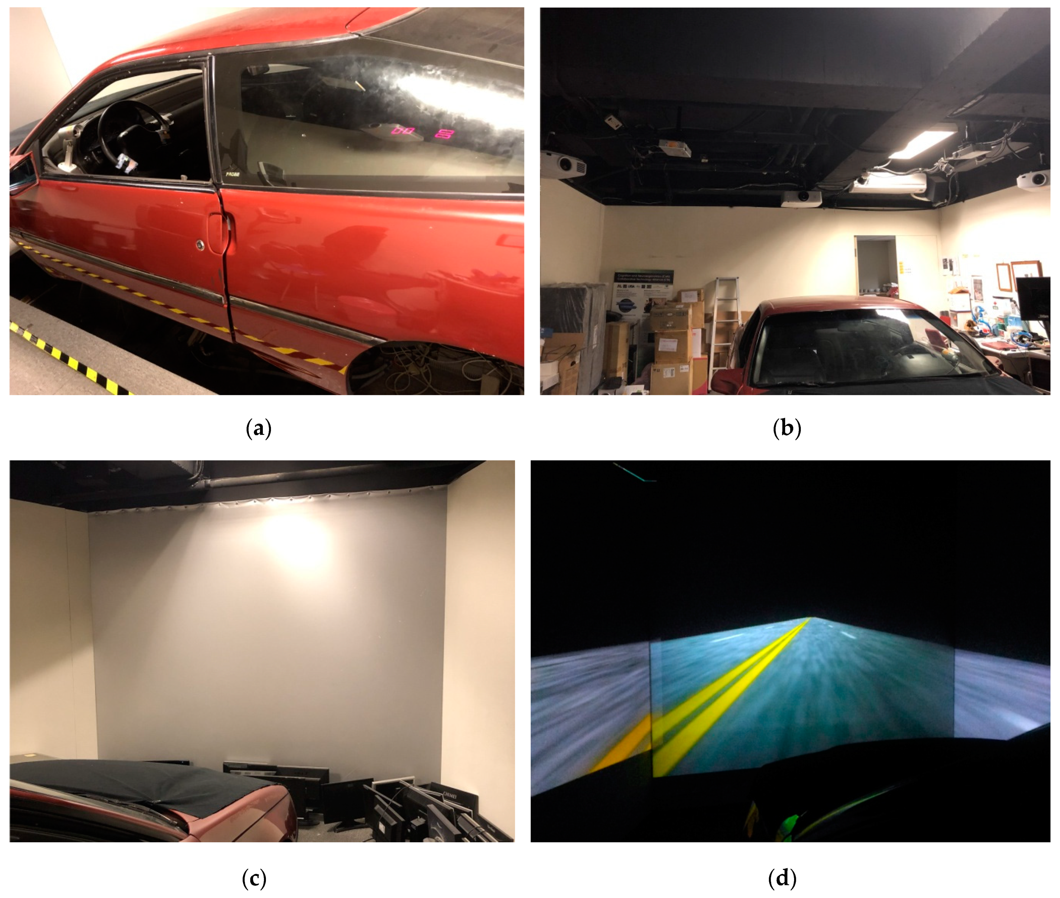
In our previous studies, to observe the subject’s drowsy state during the driving task, a virtual reality (VR)-based realistic driving environment was developed to simulate a long-term driving situation [2,13,32,33,34,35]. As shown in Figure 1, the surrounding scenes were projected from six projectors to constitute a surrounding vision. A night-time driving scene at a fixed velocity of 100 km/h on a four-lane highway is set up in the VR experiment. Before the experiment was started, participants were directed to enter the real car mounted on a motion platform and then steer the vehicle according to the instructions. All participants were required to take a 5-min pre-test session to ensure that they clearly understood the instruction and did not suffer from simulator sickness. The highway scene was connected to a physiological measuring system, where the EEG and participants’ performance were continuously and simultaneously measured and recorded.

2.2. Driving Fatigue Paradigm

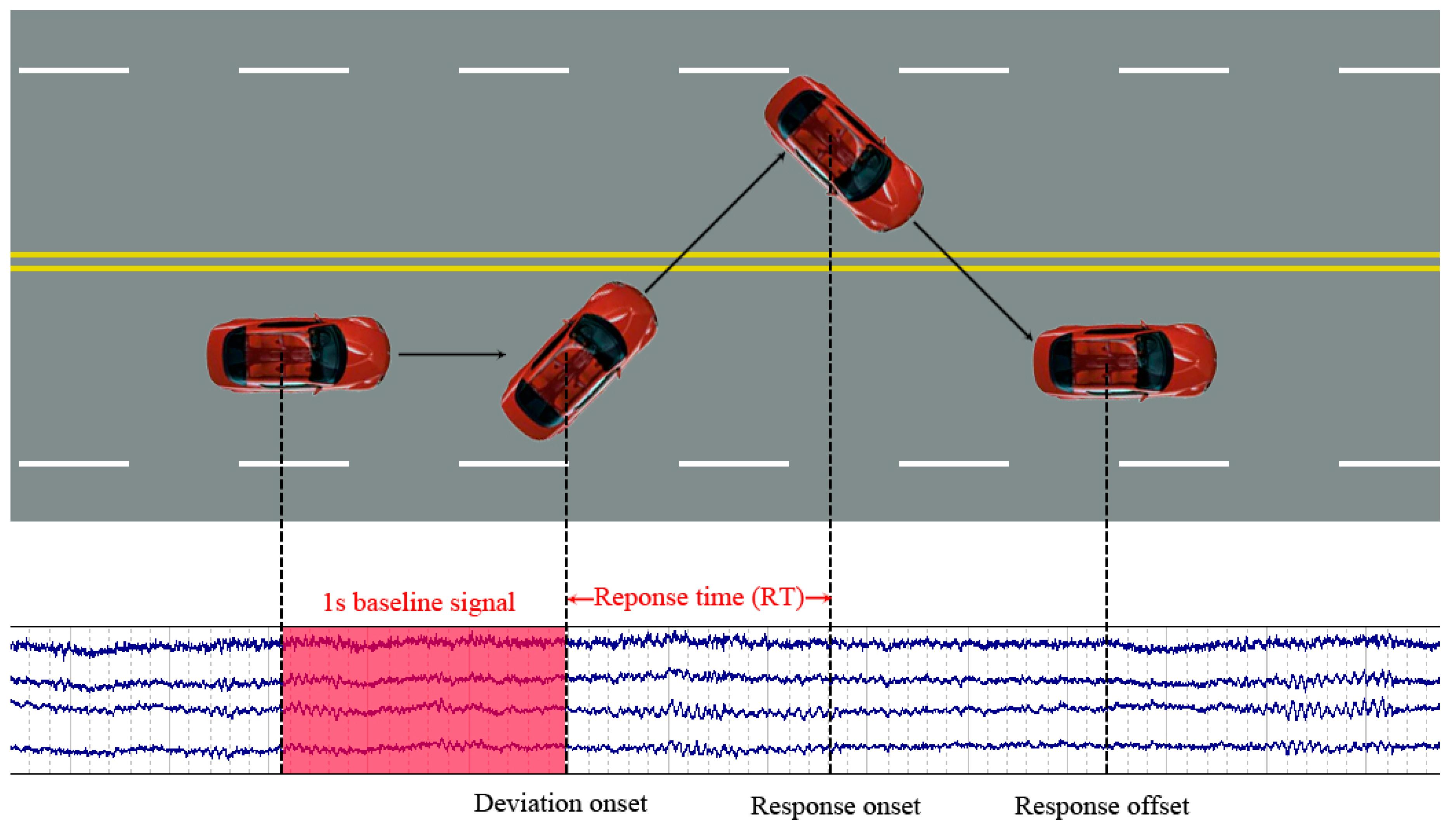
The event-related lane-keeping driving task was adopted in this study for the evaluation of the brain dynamics occurring during the driving task, as illustrated in Figure 2. The participants were instructed to perform a 90-min driving task without breaking or resting in the VR driving environment. The driving experiment began in the early afternoon (13:00–14:00) after lunch because people often feel sleepy during this time [36]. During the sustained attention driving task, the VR paradigm randomly simulated a lane-departure event that caused the car to drift away from the center of the cruising lane. The participants were required to quickly steer the car back whenever the car started to deviate from the original cruising lane. There was no feedback to wake the participants even if they did not respond to the lane-departure event. The car continued to move along the curb until the participants steered it to return to the center of the cruising lane. Figure 2 describes a complete trial in the driving paradigm that includes the one-second baseline recording, deviation onset, response onset, and response offset. The time interval between the random lane-departure event was set to 5–10 s.

2.3. Participants

Thirty-eight right-handed, healthy young adults aged 20–30 years participated in the driving experiment. All subjects were required to have a driving license and sufficient sleep in the two preceding weeks. According to self-reporting, no subject had a history of psychological disorders. Before the experiment, the subjects were asked to answer a questionnaire about their sleep patterns to ensure that they had a normal cognitive state during the driving task, and they needed to complete a consent form explaining the experimental protocol that was approved by the Institutional Review Board of the Taipei Veterans General Hospital, Taiwan. The EEG signals of the subjects were captured from a Quik-Cap (CompumedicalNeuroScan) with 32 Ag/AgCl electrodes, including 30 EEG electrodes and two reference electrodes. The EEG electrodes were placed in accordance with a modified international 10–20 system. The impedance of all electrodes was kept under 5 kΩ during the experiments.

2.4. Drowsiness Measurement

The driving performance was defined based on the response time (RT), which represented the time between the deviation onset and the response onset. As the lane-departure event occurred, it was expected that the participant would take a long time to steer the car back to the center of the cruising lane if he/she was in a drowsy state; then, the response time (RT) in the trial could be very long. By contrast, when the participant was alert, he/she could respond to the lane-departure event in a short time. Previous studies have shown that baseline EEG activity is strongly correlated with changes in RT [34]. In this study, the 1s baseline signal (red region shown in Figure 2) was used to perform the drowsy prediction based on the trial’s RT.

3. Approach

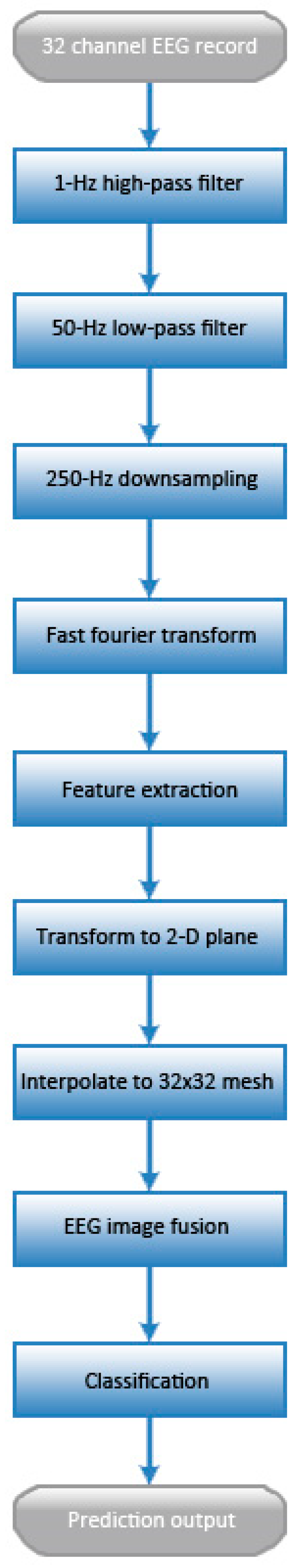
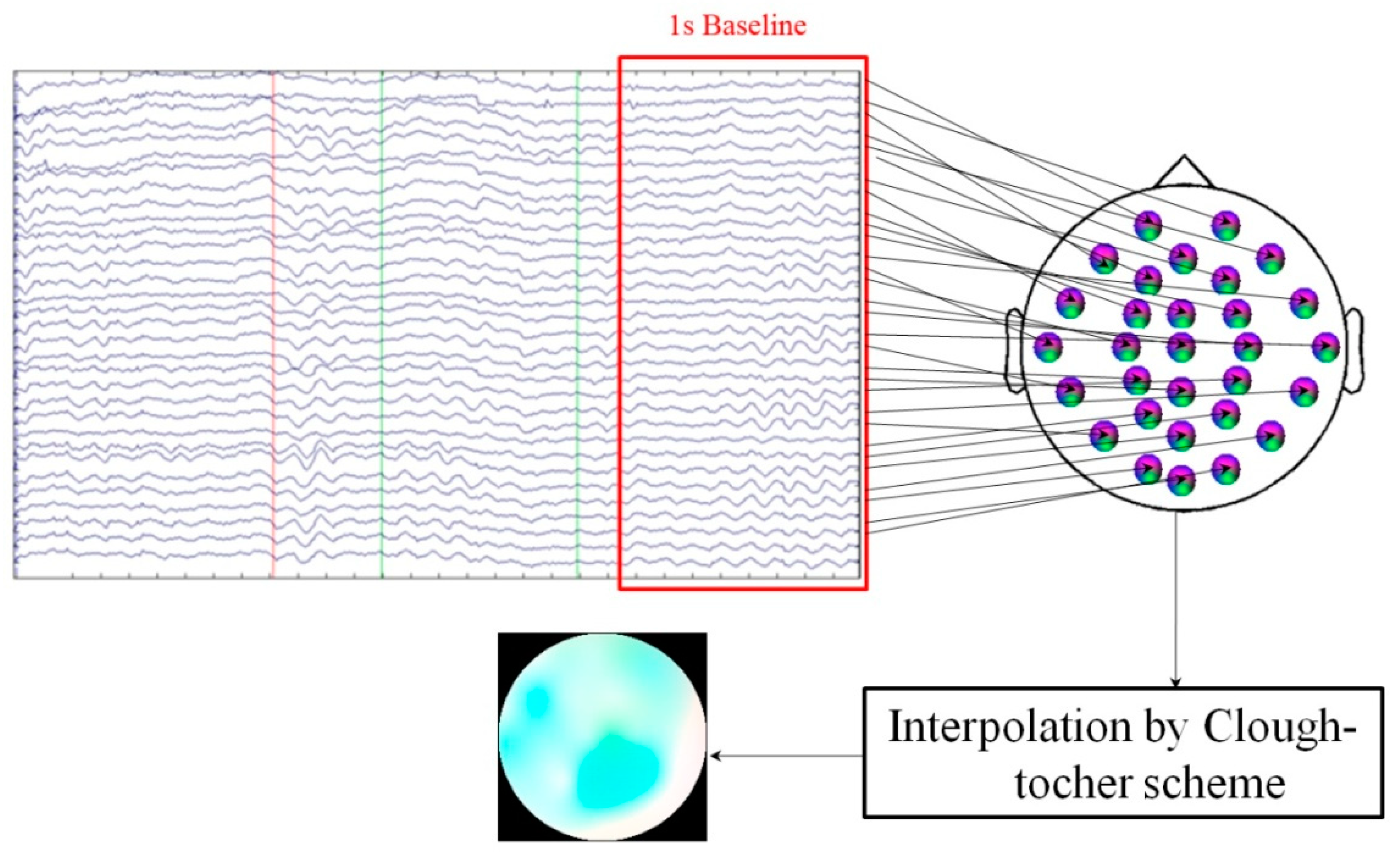
The general flowchart of our method is presented in Figure 3. Before data analysis, the acquired EEG records were processed using a 1-Hz high-pass and 50-Hz low-pass infinite impulse response filter to remove the noise and then down-sampled to 250-Hz to reduce the dimensions of the data. The power spectral activities of EEG signals were computed using FFT. To transform the EEG signal to a 2D image, we needed to address the following issues: (1) transforming the power spectrum of EEG signals to image values and (2) interpolating the points of the image data to a color image. The detailed approach is explained in the following sections.

3.1. Feature Extraction

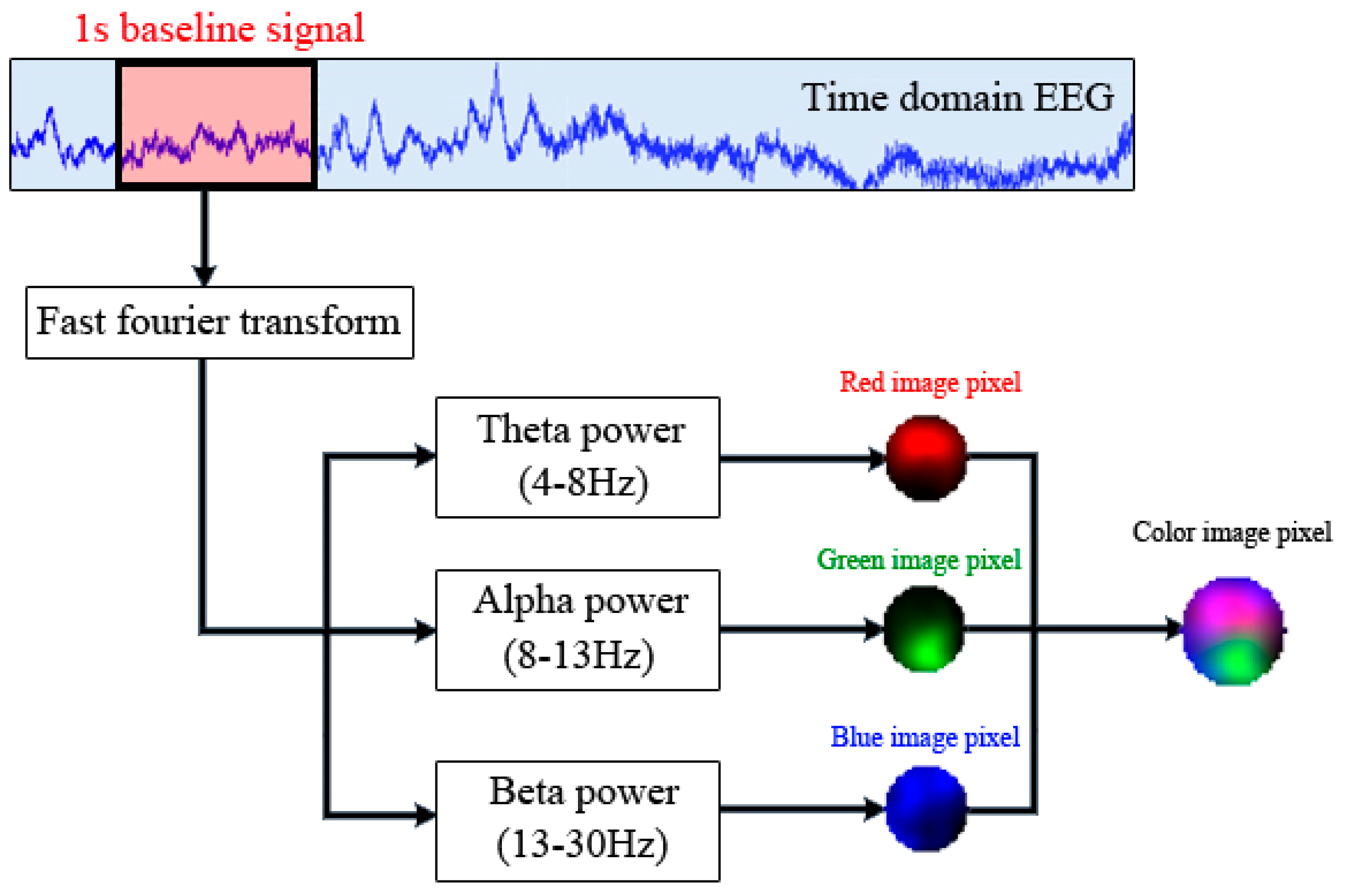
To extract the physiological features, the 30-channel time-series EEG signal was transformed into a frequency domain via a 256-point FFT. Based on the findings in previous studies [14,37,38], the frequency band in the, theta (4–8 Hz), alpha (8–13 Hz), and beta (13–20 Hz) was suitable for estimating the driver’s vigilance level. Our past studies also observed that the increasing power of theta band and alpha band had positive correlation with RT, and beta band had high correlation to kinesthetic stimuli which can affect the prediction performance [13,17]. The mean power of these frequency bands of interest was combined to form a feature vector. As depicted in Figure 4, this feature vector was considered a pixel value of the RGB image. Each channel of the colour image corresponds to a frequency band of interest.

3.2. Interpolation of the EEG Measurement to Image Pixels

As described in the previous section, we obtained 30 data points corresponding to the location of the EEG electrodes. First, we converted the magnitude of the power spectrum of the EEG signals into an image pixel value. Equation (1) shows the sigmoid function utilized to normalize the value of the EEG power spectrum to [0,1]:

$$P_t=\frac{1}{1+e^{-0.5t}},$$

(1)

where $P_t$ is the normalized image pixel value, and $t$ is the magnitude of the frequency response in the dB. Next, we needed to interpolate the scattered image data points to a color image. Figure 5 illustrates the interpolation scheme of the EEG image. The finite element method, a numerical technique that is usually applied for the approximate solution of engineering problems that are difficult to solve analytically, was adopted to perform the interpolation task. The Clough–Tocher scheme was used to interpolate a 32 × 32 mesh from the 30 image data points [39]. In this study, the EEG electrodes were placed in accordance with a modified international 10–20 system, which means that the location corresponding to each image point is known. Three topographical maps corresponding to the three frequency bands of interest were acquired by the Clough–Tocher scheme. The three spatial maps were then merged to create a 32 × 32 color image. 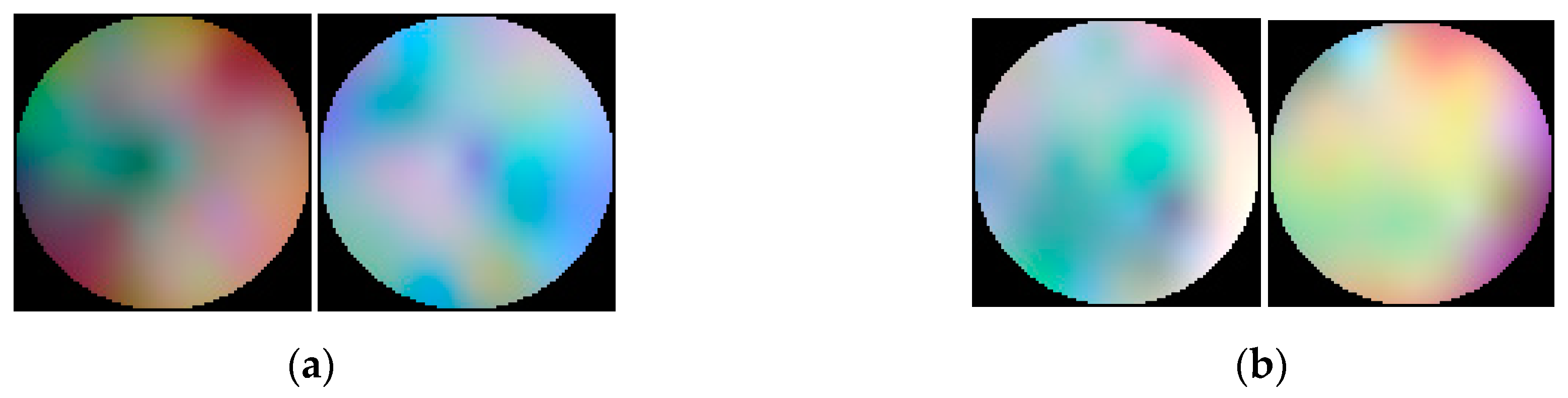Figure 6 demonstrates several samples of the EEG image.

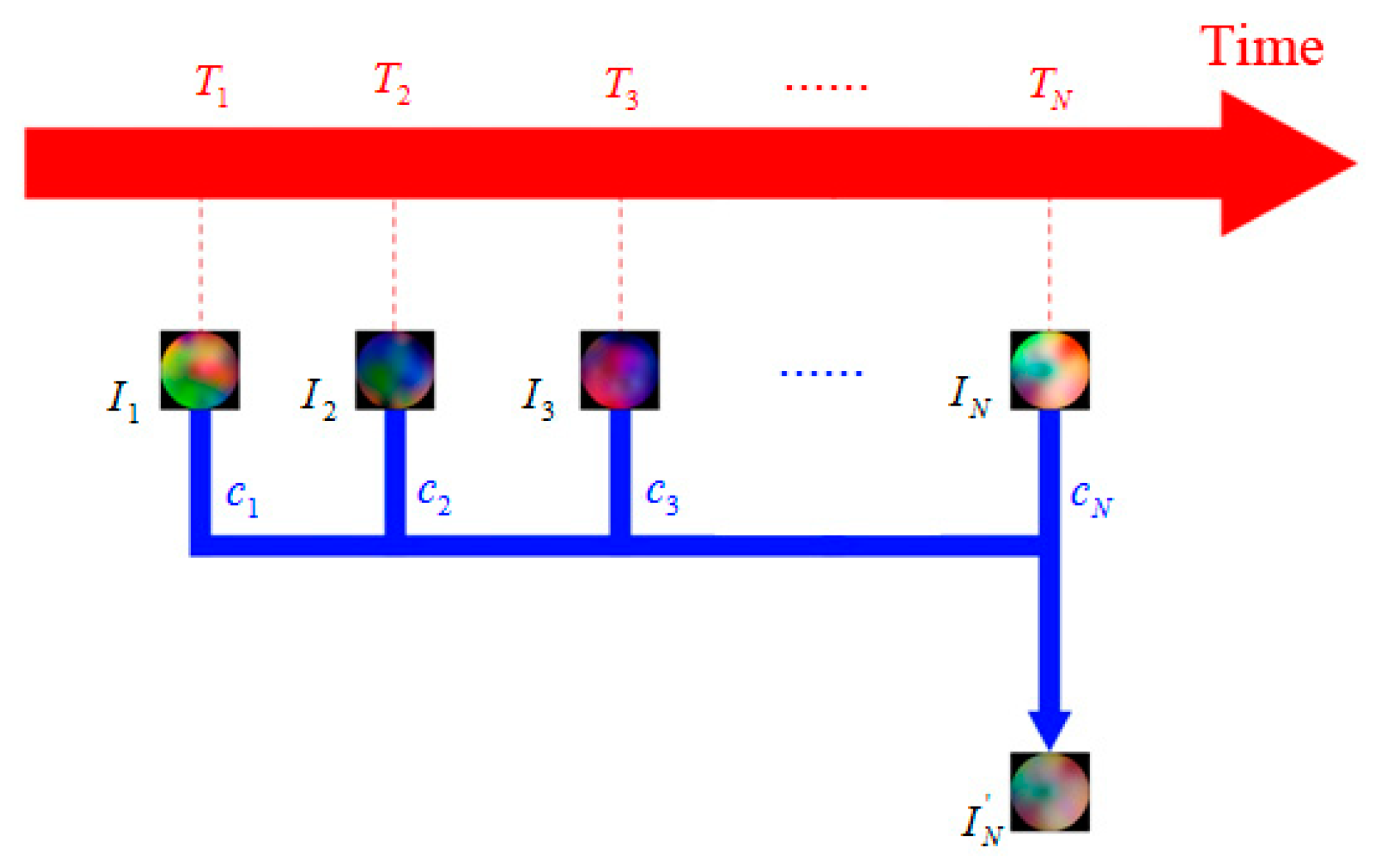
3.3. Temporal EEG Image

One of the challenges in drowsy driving prediction is that some drowsy trials may have similar patterns of the alert trials. The driving performance might not degrade immediately, even if the alertness level of the drivers begins falling, which means that drivers can respond well to lane-departure events before they fall asleep (but the drowsy pattern of the EEG has appeared). In that case, the generated EEG images between the drowsy trial and its previous alert trials can be very similar. As the drivers wake up by themselves, their vigilance level dramatically recovers, and the RT returns to the alert state; then, the EEG pattern becomes completely different from the drowsy trials. Based on these findings, the drowsy state should be estimated not only using the current trial but also by examining the previous trials. This study proposes a temporal EEG image that is generated by a linear combination of a sequence of EEG images, as shown in Equation (2):

$$\begin{array}{l}{I}_t^{\prime }={\displaystyle \sum _{t=1}^N{c}_t{I}_t}\\ {\displaystyle \sum _{t=1}^N{c}_t=1}\end{array}$$

(2)

where $I_t^{\prime }$ is the generated temporal EEG image, $I_t$ is the array of the EEG image data, c is a scalar coefficient and $c_i<c_j$ when $i<j$. $N$ in this study is set to five. Figure 7 illustrates the schematic diagram of the temporal EEG image. Instead of asingle frame EEG image $I_N$, this approach estimates the drowsiness state using $I_N^{\prime }$, which includes the information of the brain activity from multiple time points.

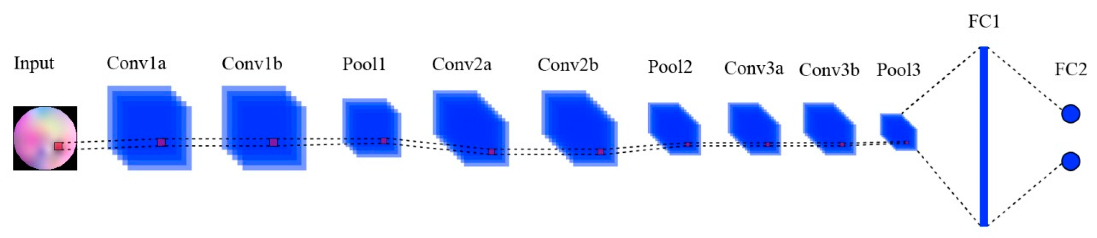
3.4. Classification Using the CNN Model

This study applies a CNN including six convolution layers, three max-pooling layers, and a layer to the classification of the input EEG image, as shown in Figure 8. A popular open source deep learning framework named Caffe is employed for implementing the CNN model [40]. The parameter setting of the overall CNN architecture is presented in

Table 1. Parameter setting of the CNN model.

Layer Name	Kernel Size	Stride	Num of Filters
Conv1a	3 × 3	1	16
Conv1b	3 × 3	1	16
Pool1	2 × 2	1	-
Conv2a	3 × 3	1	32
Conv2b	3 × 3	1	32
Pool2	2 × 2	2	-
Conv3a	3 × 3	1	32
Conv3b	3 × 3	1	32
Pool3	2 × 2	2	-
FC1	500	-	-
FC2	2	-	-

. A set of filters is used to convolve the input EEG images for feature extraction. The convolved images are then subsampled by the max-pooling layer to derive compacted features. The convolution and pooling progress are repeated several times through CNN layers. The lower-level features of the input data are extracted via the early layers, and those features are collected in the later layers to hierarchically learn the higher-level features. Finally, the acquired high-level features are concatenated and passed into the fully-connected layer for the classification. The final prediction result is determined according to the output of the fully-connected layer. We only use the alert and drowsy classes in this study, so the output size of the fully-connected layer is 2 × 1.

4. Experiment

The EEG dataset used in this study includes 10,395 alert trials and 3080 drowsy trials collected from 38 subjects. According to the suggestion of the previous research, if the drivers are fully aware of the driving situation, the average time for them to respond to the lane-departure event is approximately 0.7 s [41]. According to the previous studies [42,43,44], drivers provide poor performance when they don’t respond the lane-departure event in three times the mean alert RT. Therefore, this study adopts three times the average response time as the classification boundary of the drowsy prediction task. The EEG trials are considered as alert trials as long as their RT are less than 2.1 s. In addition, the EEG trials with an RT larger than 2.5 s are labelled as drowsy trials, and the EEG trials with an RT between 2.1 s and 2.5 s are not used in this experiment. The evaluation of our approach is performed using leave-one-subject-out cross-validation. We select the data from one subject for testing and the data from the remaining subjects for training. This process is repeated for each of the 38 subjects. To evaluate the predictive performance of the proposed method, the temporal EEG image method is compared with the single frame EEG image method—directly using the current trial of the EEG image for drowsiness prediction.

Table 2. The prediction result of the single frame EEG image and temporal EEG image.

Subject	Single Frame EEG Image			Temporal EEG Image
	Alert (%)	Drowsy (%)	Total Accuracy (%)	Alert (%)	Drowsy (%)	Total Accuracy (%)
S1	97.30	23.06	79.12	97.94	19.17	78.11
S2	88.21	20.13	52.25	82.72	29.78	53.95
S3	93.50	27.60	72.47	97.85	21.47	73.07
S4	96.76	9.30	71.85	97.79	14.19	73.33
S5	96.61	80.69	92.22	97.13	86.67	94.20
S6	96.72	84.03	93.22	98.21	96.25	97.66
S7	95.14	50.26	87.21	95.46	60.54	89.33
S8	98.30	27.69	87.31	96.42	66.15	91.60
S9	96.67	32.55	81.06	95.15	58.91	86.17
S10	96.50	12.10	80.25	96.21	8.39	79.09
S11	95.31	14.67	68.21	96.27	14.21	68.44
S12	95.60	15.80	66.30	94.50	25.71	68.90
S13	95.76	9.66	74.94	98.02	7.82	76.02
S14	92.04	17.44	80.25	96.24	16.46	83.53
S15	91.04	19.47	83.18	93.56	18.07	85.20
S16	94.10	18.25	80.62	95.06	20.00	81.62
S17	93.87	16.77	81.96	95.27	18.60	84.12
S18	92.30	16.13	85.02	92.79	16.45	85.46
S19	85.97	33.50	65.05	87.51	42.92	69.49
S20	92.40	21.44	76.24	95.15	20.17	77.94
S21	94.30	34.61	79.34	94.19	54.41	84.12
S22	92.98	21.86	76.20	94.49	21.86	77.07
S23	87.12	32.38	67.30	90.21	28.57	67.72
S24	95.68	20.28	76.46	94.83	30.35	78.27
S25	95.08	40.58	83.78	94.53	55.34	86.35
S26	92.02	37.11	85.08	91.68	48.67	86.22
S27	91.65	52.52	82.21	91.89	62.82	84.24
S28	97.60	26.50	85.55	97.29	30.25	85.73
S29	96.24	16.12	80.08	97.63	12.65	80.21
S30	94.79	12.10	74.83	95.24	13.45	75.34
S31	93.38	18.96	82.42	94.32	17.76	82.95
S32	87.57	23.57	73.37	87.92	29.76	74.78
S33	89.67	19.24	65.37	92.60	15.19	65.42
S34	89.21	25.00	84.49	90.36	22.00	85.26
S35	90.14	15.85	78.29	91.04	18.54	79.29
S36	88.33	23.57	52.43	79.65	35.63	54.75
S37	95.76	12.37	80.15	94.91	16.67	80.75
S38	69.29	40.23	53.27	52.73	53.60	53.22
Average	92.76	26.93	76.83	92.76	32.35	78.39

shows the comparison result of the temporal EEG image method and the single frame EEG image method. The average accuracy is an average of the accuracy of individual categories. It is apparent that the temporal EEG image method outperforms the single frame EEG image methods. In both methods, a similar accuracy of the alert class is given, but our approach achieves significant improvement in the accuracy of the drowsy class. Based on the aim of drowsiness prediction, the prediction rate of the drowsy class is more important than the alert class. Furthermore, the results also demonstrate that our approach has better prediction performance than the single frame EEG image method in most subjects, which proves that the improvement of our approach has universality in general users.

Table 3. The prediction result of EEGnet and HCNN.

Subject	EEGnet [45]			HCNN [28]
	Alert (%)	Drowsy (%)	Total Accuracy (%)	Alert (%)	Drowsy (%)	Total Accuracy (%)
S1	94.39	13.33	73.99	99.07	11.11	76.92
S2	84.92	24.53	52.1	90.48	17.33	50.72
S3	93.84	16.4	68.7	95.51	21.33	71.43
S4	92.79	14.19	69.8	94.23	13.95	70.75
S5	90.81	18.89	70.66	99.45	86.11	95.72
S6	88.65	20.28	69.49	98.37	93.55	96.89
S7	91.26	23.24	79.29	94.82	32.43	83.88
S8	93.21	17.69	81.17	97.08	15.38	84.05
S9	92.46	16.73	73.69	98.2	12.73	77.03
S10	89.77	20.16	76.19	92.97	16.13	77.98
S11	91.8	12.12	64.8	92.54	12.72	65.5
S12	91.75	14.91	63.16	93.12	12.5	63.12
S13	96.4	9.08	75.1	94.31	11.76	74.18
S14	90.62	15.12	78.6	96.77	14.63	83.69
S15	91.18	16.67	82.93	89.96	21.05	82.33
S16	93.46	13.81	79.21	89.44	27.84	78.41
S17	91.69	15.91	80.66	84.43	17.2	74.65
S18	92.65	17.26	81.56	88.52	11.29	81.14
S19	91.41	14.75	60.44	94.92	17.5	63.63
S20	91.52	15.25	74.01	92.42	16.95	75.1
S21	94.09	19.31	75.16	97.34	20.59	77.92
S22	86.52	19.15	70.37	89.3	18.64	72.36
S23	85.65	19.63	61.56	96.35	7.94	64.09
S24	90.76	15.25	71.37	92.16	16.31	72.68
S25	87.33	20.58	73.38	97.69	22.33	81.95
S26	87.91	17.23	78.93	90.18	36.14	83.31
S27	89.78	15.95	71.84	96.08	28.24	79.59
S28	92.19	16.5	79.14	95.83	20	82.76
S29	92.37	13.27	76.15	95.79	12.24	78.66
S30	91.32	14.03	72.52	92.7	15.13	73.82
S31	91.95	16.27	80.71	92.19	17.91	81.15
S32	91.32	21.9	75.65	90.28	16.67	73.66
S33	100	0	64.89	90.41	11.39	62.67
S34	58.14	35	56.42	86.29	20	81.34
S35	83.3	29.76	74.62	88.68	17.07	77.08
S36	100	0	43.43	88.37	22.32	51.001
S37	83.62	17.22	71.61	92.02	22.22	79.4
S38	80	20.12	46.12	87.88	13.95	46.05
Average	90.02184	16.88132	71.03737	93.05658	21.64684	74.91082

shows the evaluation result of EEGnet and hierarchical convolutional neural network (HCNN), which are CNN-based approach for EEG analysis and achieve good performance in their applications [45]. The results demonstrate that the proposed method yields superior prediction performance than EEGnet and HCNN.

5. Discussion and Conclusions

It is challenging to classify EEG data without an artifact removal process because drivers’ brain activity can change over time due to many factors, such as their mental state and body movement, which result in the temporal fluctuations of the EEG signals. However, there still contains important information associated with the drowsiness level of drivers, and thus, the temporal analysis of the EEG signals becomes a crucial issue. This study proposes a temporal EEG image algorithm that combines a sequence of EEG images to form a new EEG image that contains brain dynamics from multiple time points. Our experimental results show that the proposed method achieves good performance in the drowsiness prediction.

Support vector machines (SVMs) are also employed for comparison with our approach because they are popular classifiers for EEG analysis. In our experiment, the computational cost is expensive and a bad prediction result is obtained if we use the EEG image as the input of SVM. Thus, the power spectrum of EEG is selected as the input of the SVM. Similar to the experiment described in the previous sections, the input data do not apply any artifact removal process. The experimental results indicate that SVM provides a biased prediction result towards the alert class. That is, it always predicts an alert regardless of the input and results in a perfect detection of alert trials but no detection of drowsy trials. We found that SVM only provides meaningful prediction results in a balanced training dataset that has a similar number of alert trials and drowsy trials. In real-world applications, BCI systems usually have to perform drowsiness prediction under imbalanced-datasets, which means that SVM cannot provide reasonable reliability in real-world BCI applications.

To find a suitable CNN model for the drowsiness prediction task, this study introduces two CNN architectures for further evaluation: (1) AlexNet—a very popular CNN architecture that is larger than the CNN architecture used in this study [18], (2) 3D CNN—by performing 3D convolutions, which is capable of learning features from both spatial and temporal dimensions. For AlexNet, the EEG measurement is transformed into 227 × 227 to fit the input size of AlexNet. For 3D CNN, different from our approach using a linear combination of a sequence of EEG images, these EEG images are directly fed into the 3D CNN model since they are 3D input data. Our results show that both AlexNet and 3D CNN cannot achieve better performance than the proposed CNN architecture in the present study. That is, high-complexity CNN is not required for the drowsiness prediction task.

The detection of drowsy trials remains a challenge because different subjects have different drowsy EEG patterns. A further investigation of brain dynamics is the key to improving the prediction performance of the BCI system.

References

- Chuang, S.-W.; Ko, L.-W.; Lin, Y.-P.; Huang, R.-S.; Jung, T.-P.; Lin, C.-T. Co-modulatory spectral changes in independent brain processes are correlated with task performance. Neuroimage 2012, 62, 1469–1477. [Google Scholar] [CrossRef] [PubMed]
- Huang, C.S.; Pal, N.R.; Chuang, C.H.; Lin, C.T. Identifying changes in EEG information transfer during drowsy driving by transfer entropy. Front. Hum. Neurosci. 2015, 9, 570. [Google Scholar] [CrossRef] [PubMed]
- Liu, Y.T.; Lin, Y.Y.; Wu, S.L.; Chuang, C.H.; Lin, C.T. Brain Dynamics in Predicting Driving Fatigue Using a Recurrent Self-Evolving Fuzzy Neural Network. IEEE Trans. Neural Netw. Learn. Syst. 2015, 27, 347–360. [Google Scholar] [CrossRef] [PubMed]
- Baulk, S.D.; Reyner, L.A.; Horne, J.A. Driver sleepiness—Evaluation of reaction time measurement as a secondary task. Sleep 2001, 24, 695–698. [Google Scholar] [CrossRef]
- Banks, S.; Catcheside, P.; Lack, L.; Grunstein, R.R.; McEvoy, R.D. Low levels of alcohol impair driving simulator performance and reduce perception of crash risk in partially sleep deprived subjects. Sleep 2004, 27, 1063–1067. [Google Scholar] [CrossRef]
- Campagne, A.; Pebayle, T.; Muzet, A. Correlation between driving errors and vigilance level: Influence of the driver’s age. Physiol. Behav. 2004, 80, 515–524. [Google Scholar] [CrossRef]
- Arunkumar, N.; Ramkumar, K.; Venkatraman, V.; Abdulhay, E.; Fernandes, S.L.; Kadry, S.; Segal, S. Classification of focal and non-focal EEG using entropies. Pattern Recognit. Lett. 2017, 94, 112–117. [Google Scholar]
- Long, J.; Li, Y.; Wang, H.; Yu, T.; Pan, J.; Li, F. A hybrid brain computer interface to control the direction and speed of a simulated or real wheelchair. IEEE Trans. Neural Syst. Rehabil. Eng. 2012, 20, 720–729. [Google Scholar] [CrossRef] [PubMed]
- Xiong, Y.; Gao, J.; Yang, Y.; Yu, X.; Huang, W. Classifying driving fatigue based on combined entropy measure using EEG signals. Int. J. Control Autom. 2016, 9, 329–338. [Google Scholar] [CrossRef]
- Winkler, I.; Haufe, S.; Tangermann, M. Automatic classification of artifactual ICA-Components for artifact removal in EEG signals. Behav. Brain Funct. 2011, 7, 30. [Google Scholar] [CrossRef]
- Hyvärinen, A.; Karhunen, J.; Oja, E. Independent Component Analysis; Wiley-Interscience: New York, NY, USA, 2001. [Google Scholar]
- Tran, Y.; Craig, A.; Boord, P.; Craig, D. Using independent component analysis to remove artifact from electroencephalographic measured during stuttered speech. Med. Biol. Eng. Comput. 2004, 42, 627–633. [Google Scholar] [CrossRef] [PubMed]
- Lin, C.-T.; Wu, R.-C.; Liang, S.-F.; Chao, W.-H.; Chen, Y.-J.; Jung, T.-P. EEG-based drowsiness estimation for safety driving using independent component analysis. IEEE Trans. Circuits Syst. I Regul. Pap. 2005, 52, 2726–2738. [Google Scholar]
- Jung, T.P.; Humphries, C.; Lee, T.W.; Makeig, S.; McKeown, M.J.; Iragui, V.; Sejnowski, T.J. Extended ICA removes artifacts from electroencephalographic recordings. Adv. Neural Inf. Process. Syst. 1998, 10, 894–900. [Google Scholar]
- Garipelli, G.; Chavarriaga, R.; R Millán, J. Single trial analysis of slow cortical potentials: A study on anticipation related potentials. J. Neural Eng. 2013, 10, 036014. [Google Scholar] [CrossRef][Green Version]
- Pfurtscheller, G.; Neuper, C. Motor imagery and direct brain- computer communication. Proc. IEEE 2001, 89, 1123–1134. [Google Scholar] [CrossRef]
- Chuang, C.H.; Lai, P.C.; Ko, L.W.; Kuo, B.C.; Lin, C.T. Driver’s cognitive state classification toward brain computer interface via using a generalized and supervised technology. In Proceedings of the 2010 International Joint Conference on Neural Networks (IJCNN), Barcelona, Spain, 18–23 July 2010; pp. 1–7. [Google Scholar]
- Tabar, Y.R.; Halici, U. A novel deep learning approach for classification of EEG motor imagery signals. J. Neural Eng. 2016, 14, 016003. [Google Scholar] [CrossRef]
- Carvalho, S.R.; Filho, I.C.; Resende, D.O.; Siravenha, A.C.; De Souza, C.R.B.H.; Debarba, B.D.; Gomes, R.; Boulic, A. Deep Learning Approach for Classification of Reaching Targets from EEG Images. In Proceedings of the 2017 30th SIBGRAPI Conference on Graphics, Patterns and Images (SIBGRAPI), Niteroi, Brazil, 17–20 October 2017. [Google Scholar]
- Hinton, G.; Deng, L.; Yu, D.; Dahl, G.A.; Mohamed, N.; Jaitly, A.; Senior, V.; Vanhoucke, P.; Nguyen, T.; Sainath, B. Kingsbury, Deep neural networks for acoustic modeling in speech recognition. IEEE Signal. Process. Mag. 2012, 29, 82–97. [Google Scholar] [CrossRef]
- Krizhevsky, A.; Sutskever, I.; Hinton, G. Imagenet classification with deep convolutional neural networks. In Proceedings of the NIPS, Doha, Qatar, 12–15 November 2012. [Google Scholar]
- Taigman, Y.; Yang, M.; Ranzato, M.; Wolf, L. DeepFace: Closing the Gap to Human-Level Performance in Face Verification. In Proceedings of the IEEE Conference on Computer Vision and Pattern Recognition (CVPR), Columbus, OH, USA, 24–27 June 2014. [Google Scholar]
- Sun, Y.; Wang, X.; Tang, X. Deep Learning Face Representation from Predicting 10,000 Classes. In Proceedings of the IEEE Conference on Computer Vision and Pattern Recognition (CVPR), Columbus, OH, USA, 24–27 June 2014. [Google Scholar]
- Karpathy, A.; Toderici, G.; Shetty, S.; Leung, T.; Sukthankar, S.; Li, F.-F. Large-scale video classication with convolutional neural networks. In Proceedings of the IEEE Conference on Computer Vision and Pattern Recognition (CVPR), Columbus, OH, USA, 24–27 June 2014. [Google Scholar]
- Jirayucharoensak, S.; Pan-Ngum, S.; Israsena, P. Eeg-based emotion recognition using deep learning network with principal component based covariate shift adaptation. Sci. World J. 2014, 2014, 627892. [Google Scholar] [CrossRef]
- Zheng, W.-L.; Zhu, J.-Y.; Peng, Y.; Lu, B.-L. EEG-based emotion classification using deep belief networks. In Proceedings of the 2014 IEEE International Conference on Multimedia and Expo (ICME), Chengdu, China, 14–18 July 2014. [Google Scholar]
- Hosseini, M.-P.; Soltanian-Zadeh, H.; Elisevich, K.; Pompili, D. Cloud-based deep learning of big eeg data for epileptic seizure prediction. In Proceedings of the 2016 IEEE Global Conference on Signal and Information Processing (GlobalSIP), Washington, DC, USA, 7–9 December 2016. [Google Scholar]
- Li, J.; Zhang, Z.; He, H. Hierarchical convolutional neural networks for EEG-based emotion recognition. Cogn. Comput. 2017, 10, 368–380. [Google Scholar] [CrossRef]
- Bashivan, P.; Rish, I.; Yeasin, M.; Codella, N. Learning representations from EEG with deep recurrent-convolutional neural networks. Int. Conf. Learn. Represent. 2016, 1511, 06448. [Google Scholar]
- Emami, A.; Kunii, N.; Matsuo, T.; Shinozaki, T.; Kawai, K.; Takahashi, H. Seizure detection by convolutional neural network-based analysis of scalp electroencephalography plot images. NeuroImage Clin. 2019, 22, 101684. [Google Scholar] [CrossRef]
- Comaniciu, A.; Najafizadeh, L. Enabling Communication for Locked-in Syndrome Patients using Deep Learning and an Emoji-based Brain Computer Interface. In Proceedings of the 2018 IEEE Biomedical Circuits and Systems Conference (BioCAS), Cleveland, OH, USA, 24 December 2018. [Google Scholar]
- Lin, F.-C.; Ko, L.-W.; Chuang, C.-H.; Su, T.-P.; Lin, C.-T. Generalized EEG-based drowsiness prediction system by using a self-organizing neural fuzzy system. IEEE Trans. Circuits Syst. I Reg. Pap. 2012, 59, 2044–2055. [Google Scholar] [CrossRef]
- Huang, R.-S.; Jung, T.-P.; Delorme, A.; Makeig, S. Tonic and phasic electroencephalographic dynamics during continuous compensatory tracking. NeuroImage 2008, 39, 1896–1909. [Google Scholar] [CrossRef] [PubMed]
- Chuang, C.H.; Ko, L.W.; Jung, T.P.; Lin, C.T. Kinesthesia in a sustained-attention driving task. Neuroimage 2014, 91, 187–202. [Google Scholar] [CrossRef] [PubMed][Green Version]
- Lin, C.T.; Wu, R.C.; Jung, T.P.; Liang, S.F.; Huang, T.Y. Estimating Driving Performance Based on EEG Spectrum Analysis. EURASIP J. Appl. Signal. Process. 2005, 19, 3165–3174. [Google Scholar] [CrossRef]
- Ueno, H.; Kaneda, M.; Tsukino, M. Development of drowsiness detection system. In Proceedings of the VNIS’94-1994 Vehicle Navigation and Information Systems Conference, Yokohama, Japan, 6 August 2002. [Google Scholar]
- Jap, B.T.; Lal, S.; Fischer, P.; Bekiaris, E. Using EEG spectral components to assess algorithms for detecting fatigue. Expert Syst. 2009, 36, 2352–2359. [Google Scholar] [CrossRef]
- Bashivan, P.; Bidelman, G.M.; Yeasin, M. Spectrotemporal dynamics of the EEG during working memory encoding and maintenance predicts individual behavioral capacity. Eur. J. Neurosci. 2014, 40, 3774–3784. [Google Scholar] [CrossRef]
- Alfeld, P. A trivariate clough-tocher scheme for tetrahedral data. Comput. Aided Geom. Des. 1984, 1, 169–181. [Google Scholar] [CrossRef]
- Jia, Y.; Shelhamer, E.; Donahue, J.; Karayev, S.; Long, J.; Girshick, R.; Guadarrama, S.; Darrell, T. Caffe: Convolutional architecture for fast feature embedding. arXiv 2014, arXiv:1408.5093. [Google Scholar]
- Marc, G. How Long Does It Take to Stop? Methodological Analysis of Driver Perception-Brake Times. Transp. Hum. Factors 2000, 2, 195–216. [Google Scholar]
- Lin, C.T.; Huang, K.C.; Chuang, C.H.; Ko, L.W.; Jung, T.P. Can arousing feedback rectify lapses in driving? Prediction from EEG power spectra. J. Neural Eng. 2013, 10, 056024. [Google Scholar] [CrossRef] [PubMed]
- Huang, K.C.; Jung, T.P.; Chuang, C.H.; Ko, L.W.; Lin, C.T. Preventing lapse in performance using a drowsiness monitoring and management system. In Proceedings of the 2012 Annual International Conference of the IEEE Engineering in Medicine and Biology Society, San Diego, CA, USA, 12 November 2012. [Google Scholar]
- Lin, C.-T.; Huang, K.-C.; Chao, C.-F.; Chen, J.-A.; Chiu, T.-W.; Ko, L.-W.; Jung, T.-P. Tonic and phasic EEG and behavioral changes induced by arousing feedback. NeuroImage 2010, 52, 633–642. [Google Scholar] [CrossRef] [PubMed]
- Lawhern, V.J.; Solon, A.J.; Waytowich, N.R.; Gordon, S.M.; Hung, C.P.; Lance, B.J. EEGNet: A compact convolutional neural network for EEG-based brain computer interfaces. J. Neural Eng. 2018, 15, 056013. [Google Scholar] [CrossRef] [PubMed]
© 2019 by the authors. Licensee MDPI, Basel, Switzerland. This article is an open access article distributed under the terms and conditions of the Creative Commons Attribution (CC BY) license (http://creativecommons.org/licenses/by/4.0/).