The Teager-Kaiser Energy Cepstral Coefficients as an Effective Structural Health Monitoring Tool

Featured Application

This paper presents a damage sensitive feature, the Teager-Kaiser Energy Cepstral Coefficients (TECCs), which can be used to train a Machine Learning algorithm to perform damage detection and Structural Health Monitoring (SHM) on complex buildings and/or mechanical systems.

Abstract

Recently, features and techniques from speech processing have started to gain increasing attention in the Structural Health Monitoring (SHM) community, in the context of vibration analysis. In particular, the Cepstral Coefficients (CCs) proved to be apt in discerning the response of a damaged structure with respect to a given undamaged baseline. Previous works relied on the Mel-Frequency Cepstral Coefficients (MFCCs). This approach, while efficient and still very common in applications, such as speech and speaker recognition, has been followed by other more advanced and competitive techniques for the same aims. The Teager-Kaiser Energy Cepstral Coefficients (TECCs) is one of these alternatives. These features are very closely related to MFCCs, but provide interesting and useful additional values, such as e.g., improved robustness with respect to noise. The goal of this paper is to introduce the use of TECCs for damage detection purposes, by highlighting their competitiveness with closely related features. Promising results from both numerical and experimental data were obtained.

1. Introduction

Damage detection and Structural Health Monitoring (SHM) indicate the field of engineering that is involved in the assessment of the structural integrity for civil, mechanical, and aerospace applications, among others [1]. More specifically, vibration-based SHM [2] deals with the structural response, as recorded by means of a sensor network, to extract damage-related features from its free or forced oscillations. In this context, recent years have seen a continuous surge of interest in Machine Learning (ML) algorithms, as they are perfectly suited for damage detection [3], if this is seen from a Pattern Recognition/Novelty Detection standpoint [4]. The concept is simple: by knowing the current state of a system (which is usually undamaged, but can be indistinctly previously damaged, as long as it is stable and not dramatically changing under “normal” conditions), a baseline can be defined. This is performed by training a “normality” model via ML techniques over the features that were extracted from the known set of data. Subsequently, the structural response from other scenarios can be labelled as divergent from this model or not by regarding the value of a distance metric between its current response and the baseline model. One can refer to the previously cited book of Farrar & Worden for a detailed description of the basics of ML for SHM [1].

Some damage-related features (also known as damage sensitive features, DSFs) are needed for training and testing a Machine Learning algorithm. Eventually, DSFs need to be as low in dimensionality as possible, since a very large number of cases is required for the training phase, preserving the relevant information while discarding unrelated effects. However, feature selection is a concern much broader than its SHM applications. One of the fields where it has seen a major development is in speech, speaker, and language recognition.

Virtual assistants, human-like speech synthesis, and audio indexing are all examples of ML applied to Speech Processing for Artificial Intelligence (AI) purposes. Other applications are countless: automatic transcription to text and conversational human-machine interfaces are the most obvious uses of speech recognition. Speaker recognition, i.e., the process of automatically predicting the identity of the speaker by a given utterance, is used for voice biometric authentication, telephone-based services, speaker diarisation, and forensic activities. Finally, language recognition finds its main applications in emergency call routing, spoken language translation, and audio surveillance, to cite a few. Speaker and language recognition rely on similar techniques, as they mostly share the same problems: preprocessing the signal, extracting its relevant features, and representing them by means of statistical models.

There are no conceptual impediments for the application of the related techniques for vibration-based SHM if acceleration time histories (THs) from the structure of interest are considered instead of audio samples. As for speaker recognition, distinctive traits, related to specific phenomena of interest, have to be spotted and discerned from uninteresting effects. On the one hand, mechanical vibrations and biomedical signals show the same issues, such as changing content along time (both frequency- and amplitude-wise) during dynamic excitation, which cannot be properly depicted by means of Discrete Fourier Transform (DFT) [5], and thus require joint time-frequency analysis techniques for a two-dimensional, time-vs-frequency representation [6,7], such as the one obtained via wavelet analysis [8,9,10,11]. On the other hand, speech signals present some difficulties—such as different duration between samples, unknown input, and high level of non-stationarity—which are generally much less impelling for civil and mechanical structures rather than in biological systems [12]. Indeed, it is possible to figure the human speech production system out as a control system, where the plant dynamics are related to the vocal tract characteristics, while the constriction and airflow mechanisms are the biological counterparts of the controller. In this sense, the analogy with structural vibrations is straightforward. Some other examples of contamination between the speech processing techniques and structural health monitoring include some recent works on Wavelet Levels (WLs), on Hilbert-Huang Transform (HHT), and on Empirical Mode Decomposition (EMD) [13,14]. Other proposals include well-known techniques, such as the Continuous Wavelet Transform (CWT), the Unscented Kalman Filter (UKF), and the Blind Source Separation (BSS) [5].

By far, the cepstrum [15] has been the main contribution to the field, being often coupled with other techniques, such as autoregressive moving-average (ARMA) models [16] or directly applied for the cepstral editing of signals [17,18]; an extensive review of the uses of cepstral features for the monitoring of mechanical (non-biological) vibrations can be found in [19].

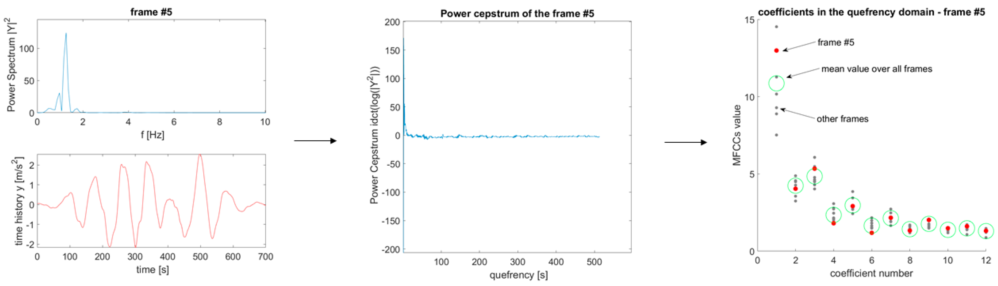
Mel-Frequency Cepstral Coefficients (MFCCs) are an example of low-dimensional, fixed dimension feature vectors defined into a cepstral framework, which are very effective in speech processing and already successfully tested as DSFs for mechanical systems [20,21] and subsequently refined [22]. MFCCs proved to be apt in detecting damage in experimental and numerically simulated data for simpler structural elements and in more complex cases, such as historic masonry buildings. However, this feature is not free of issues; one of the major problems of MFCCs is how they can be swayed by additive noise with relative ease. Indeed, log-mel-amplitudes are influenced by the low-energy component of the signal and this is more strongly evident in the first MF cepstral coefficient.

Similarly to the MFCCs, the Teager-Kaiser Energy Cepstral Coefficients (TECCs) were first introduced in the ambit of Speech Recognition in 2005 by Dimitriadis et al. [23], relying on the Kaiser definition of the Teager Energy Operator [24]. The process for their extraction is two-stepped. Firstly, the signal is filtered through a dense non-constant-Q Gammatone filterbank (details will follow shortly), which replaces the triangular filters utilised in the standard MFCCs approach. This initial step is shared with other closely related alternatives, such as, specifically, the Gammatone Cepstral Coefficients (GTCCs) [25], which have also been tested here in this work. Secondly, the short-time average of the output of the previously mentioned Teager-Kaiser Energy (TKE) Operator is computed. A deeper discussion for both MFCCs and TECCs is postposed to the respective subsections; it is important to remark here how the proposed TECC-based method relies on the TKE operator, which, in turn, is the basis of several time-frequency analysis approaches for the estimation of instantaneous amplitude and frequency [26]. These techniques already proved to be efficient in other fields of signal processing apart speech analysis and very recently they have been successfully applied to Structural Health Monitoring. For instance, the TKE has been combined with deep belief networks for the fault diagnosis of reciprocating compressor valves [27] and with least-squares support vector machine (LS-SVM) classifiers to detect bearing fault [28]. Nevertheless, its use is still very limited and few applications are reported in the literature.

The proposed TECC-based approach has been tested on two numerical and one experimental case studies. The first numerical case is a Finite Element (FE) model that represents the Santa Maria and San Giovenale Cathedral bell tower in Fossano, Italy, which is a structure of relevant importance for cultural heritage and it has been deeply investigated in the literature (for instance, see [29]). This is representative of historical masonry buildings, which noteworthy often present several structural problematics and require proper monitoring [30], especially in the case of high-rise medieval structures [31,32]. The second case study regards the spar of the high-aspect-ratio (HAR) prototype wing XB-1 studied in [33]. This case also presents its own difficulties, arising from the high flexibility of the cantilevered structure. The experimental data that are described in [21] have also been used for comparison. In this last case study, the damage is modelled as a breathing crack mechanism, introducing a source of nonlinearities often encountered in damaged structures, where the presence of crack often results in nonlinear behaviour [34,35]. As a benchmark, the original five alternative methods that were proposed in [21] and the six new closely-related variants described in [22] have also been applied to the numerical and experimental data; the results show interesting improvements.

It is important to stress how the choice of different structural systems, materials, and damage mechanisms for this methodology’s validation is intended to show its reliability for novelty detection in a wide range of applications and conditions, as “damage” (in the broader sense possible) might manifest itself in many different ways, also depending on the specific constructional material [36], and these different occurrences may not be all similarly easy to detect—especially in larger structures with complicated geometries.

The outline of this paper is as following: in Section 2, the needed background for a full comprehension of the context is recalled. The algorithm that is utilised for damage detection is described in Section 3. In Section 4, the numerical case studies are presented. Section 5 briefly describes the experimental data used for further validation. A comparison with previous works and similar alternatives is also proposed in the Results Section, and Conclusions follow.

2. Theoretical Background

The novel method here proposed for SHM purposes, based on the Teager-Kaiser Energy Cepstral Coefficients (TECCs), requires some previous knowledge regarding the definitions of cepstrum, quefrency [37], and the melody-frequency scale (also abbreviated as the mel-scale) [38]. This Section is intended to also provide a basic common ground for non-experts in signal and speech processing, not familiar with the jargon, and to establish some definitions before continuing. For the sake of better comprehensibility, the discussion is sequenced here into the following subsections: cepstral analysis, a brief recall about MFCCs, some hints about their (many) variants, and finally the description of the TECCs themselves.

2.1. Cepstral Analysis

A somehow basic but effective description of the cepstrum (that can be applied to both its power and complex definitions) is the “spectrum of the spectrum on logarithmic amplitude axis” [39], as it is computed as the inverse transform of the logarithm of its estimated spectrum. First described in [37], its original and main use is for pitch detection and determination [40], but in the years it has found plenty of applications in speech processing, such as for the estimation of harmonics-to-noise ratios [41]. Resorting to the cepstrum rather than the standard frequency spectrum gives some interesting advantages, mainly the possibility to easily discern and eventually edit off uninteresting harmonics. Some slightly different definitions exist, such as e.g., the discrete complex cepstrum with unwrapped phase, which are useful for time-frequency analysis purposes [42]. Preserving the phase information, the complex extension of the cepstrum allows for reconstructing the original time-dependent signal; however, for the purpose of this research, the definition of the power cepstrum is more convenient. Analytically, this can be defined by resorting to the direct and inverse z-trasform definitions, as ([43], Chapter 24)

$$\widehat{f}\triangleq {\left[{\mathcal{Z}}^{-1}\left\{\log \left({\left|H\left(z\right)\right|}^2\right)\right\}\right]}^2={\left[\frac{1}{2\pi j}{{\displaystyle \oint }}_{{\mathsf{\Gamma }}_c}^{ }\log \left({\left|H\left(z\right)\right|}^2\right) z^{n-1}dz\right]}^2$$

(1)

where ‘^’ denotes the power cepstrum of function $f$, ${\mathcal{Z}}^{-1}(·)$ is the inverse z-transform operator, $H\left(z\right)=\mathcal{Z}\left(f\right)$ represents the z-transform of an ordered, discretised time sequence $f=x\left[n\right]$, and $n$ indicates the specific time instant; the contour of integration, ${\mathsf{\Gamma }}_c$, lies within an annular region where $H\left(z\right)$ is defined as analytic and single-valued. Evaluating Equation (1) on the unit circle, the problem is reconducted to the Fourier domain, and it can be restated as

$$\widehat{f}={\left[\frac{1}{2\pi }{{\displaystyle \int }}_{-\pi }^{\pi }\log \left({\left|H\left(\omega \right)\right|}^2\right) e^{j\omega t}dt\right]}^2$$

(2)

For an angular frequency $\omega =2\pi f$ and the Discrete Fourier Transform $H\left(\omega \right)$. The basic idea exploited is the concept of homomorphic deconvolution, i.e., separating different components of one given signal, if $f$ itself is made up by a convolution of some distinct underlying signal components. With respect to the simple, more common Fourier Transform in the frequency domain, this process allows for better discerning between the content of interest and unnecessary/unrelated influences, disturbances or echoes, as convolution in time domain becomes summation in cepstral domain. Thus, thanks to the frequency-warping, the cepstral response simultaneously incorporates properties from both the time and the frequency domains. Please note that, due to direct and inverse transform, the measurement unit is the same as the departing one i.e., time expressed in seconds; nevertheless, $\widehat{f}$ cannot be considered to be an ordered time series, because of the warping. Further details can be found in [15]. However, the cepstrum of a signal maintains its same dimensionality, without any gain in conciseness with respect to raw THs. Thus, specific features, i.e., the Cepstral Coefficients (CCs), have to be extracted from it.

2.2. Cepstral Coefficients (CCs) and Mel-Frequency CCs

The Cepstral Coefficients (CCs) can be extracted from the cepstrum of a signal. In the field of speech and sound processing, the mel-scale is intensively used for this purpose, by rearranging the cepstrum in a nonlinear log-like scale of frequency. The idea is generally credited to the works of Mermelstein [44] and Bridle and Brown [45], and it has since then been developed to become a standard in speech processing.

The mel-scale is a purely empirically definition, being intended to mimic the auditory system of the human hear, which is a nonlinear sensing device with almost logarithmically spaced intervals of equivalent perception. The definition of its base unit, the Mel, is one-thousandth of the pitch (℘) of a simple tone with a 40 dB amplitude above the auditory threshold and a frequency that is equal to 1000 Hz [38,46]. The reason behind the thresholding lies in several experimental investigations (such as [47] to name one), which proved that speech processing linear-like for small spectral values and logarithmic-like for large ones yield to more robust identifications with data affected by additive or convolutional artificial noise. Obviously, this definition is very specific, perceptual, and suited for the aim of emulating the human ear. Nevertheless, this was found from previous studies to be apt for SHM purposes; this might be explained by its logarithmic-like spacing, which is recurrent in many natural events not limited to speech production and perception [21]. Another point of relevance is that the definition itself is perceptual, psychoacoustical, and based on perceived equidistance between subsequent pitches; thus, it is not directly provided with a mathematical formulation. Of the many concurrent analytical definitions for the Mel–Hertz conversion, the most commonly accepted one is the variant proposed by Fant in [48]. Other alternative definitions exist; a comparative study was performed by Umesh et al. in [49].

The procedure to extract MFCCs from a non-stationary recorded signal of interest are the following: (i) framing of the signal into more stationary tracts; (ii) windowing of the frames; (iii) computation of the Power Spectral Density (PSD) in the frequency domain; (iv) frequency warping to re-order the discrete power spectrum in the melody-frequency scale (Mel-scale); and finally, (v) L-points inverse Discrete Cosine Transform (iDCT). This last passage can be also performed by means of inverse Discrete Fourier Transform (iDFT), but iDCT is more technically convenient as more adherent to the Karhunen–Loève Transform. When considering (arbitrarily) $L-1$ coefficients to be extracted and $M$ critical bands, the resulting array of MFCCs, $\mathit{c}\in {ℝ}^{L \times 1}$, can be defined as

$$\begin{array}{c}c\left[l\right]={{\displaystyle \sum }}_{m=0}^{M-1}{a}_m\log \left(H_{\mathrm{mel}}\left[m\right]\right)\cos \left(\frac{\pi \left(2l+1\right)m}{2M}\right),\\ l=0,1,\dots ,L-1, a_m=\{\begin{array}{c}\frac{1}{M} if m=0 \\ \frac{2}{M} if m\ge 1\end{array}\end{array}$$

(3)

where $a_m$ is the amplitude multiplying the m-th point of the mel-spectrum $H_{\mathrm{mel}}\left[m\right]$. The procedure is illustrated for the example of frame #5 in Figure 1.

2.3. Similar Scales and Features Investigated

While vastly predominant in the common use, the mel-scale is not the sole nonlinear scale viable. Other options proposed in the literature include the Bark Scale [50] and the Equivalent rectangular bandwidth (ERB)-rate scale [51], to cite the two main competitors. In both cases, several Hertz–Bark/Hertz–ERB relationships were proposed in an analytical form, similarly to the Mel-Scale, as defined in [52] and in [53], respectively. Some of these alternatives, such as the Bark-Frequency Cepstral Coefficients (BFCCs) [54], have also been recently tested by the Authors for SHM purposes. In this context, three novel scales, namely, the Energy COntent-based MMFCCs (ECO-MMFCCs), the MOdal Frequency-centred MMFCCs (MO-MMFCCs), and the LOw-Frequency Restricted MMFCCs (LO- MMFCCs) have been recently proposed [22].

Apart from different psychoacoustical, Mel-like scales as the ones just mentioned, non-triangular weighting functions can also be used, such as gammatone filters [55]. Additionally, the acceleration THs can be pre-processed before applying the extraction procedure. An option is the mentioned Teager-Kaiser Energy (TKE) Operator. This, combined with the Gammatone filters, is the core of the method proposed in this work and will be better detailed in the two next subsections.

To sum up and for comparison with the previous studies, Figure 2 reports a pictorial representation of the tested approaches.

2.4. Advantages Over the Auto-Regressive Model Coefficients

The MFCCs, TECCs, and similar cepstral-based features can be compared to other DSFs to better describe their advantages. As done in [21], the discussion is here focused on the Auto-Regressive Model (AR) Coefficients, which are a classic feature widely used for SHM purposes [3,4]. An AR model of order p can be defined (for a time-discrete signal $x\left[n\right]$), as

$$x\left[k\right]={{\displaystyle \sum }}_{j=1}^p{a}_{j}x\left[k-1\right]+{ϵ}_k$$

(4)

With $x\left[k\right]$ being the signal value at the $k$-th integer multiple of the sampling interval $\mathsf{\Delta }t$, $a_j$ the $j$-th AR coefficient, and ${ϵ}_k$ the modelling error at $k\mathsf{\Delta }t$. The Akaike Information Criterion (AIC) can be used to select a proper value of $p$ to both prevent over- and under-fitting (i.e., to have a model complete enough to describe properly the observed data, but not unnecessarily overcomplicated), as

$$AIC\left(p\right)=n\left(\ln \left({\sigma }_p^2\right)+1\right)+2p$$

(5)

where $n$ is the total amount of estimated data point, $p$ is the specific order under investigation, and $\ln \left({\sigma }_p^2\right)$ is the natural logarithm of the mean of the sum of squared residual errors ${ϵ}_k$ between the model and the data at any data point.

However, with respect to AR coefficients, the cepstral features have the following useful qualities: (1) they do not require a somehow arbitrary definition of the model order (even if some arbitrariness does still exist in the definition of the $L-1$ coefficients to be extracted from the $M$ critical bands); (2) their results are much less affected by the choice of $L$ and $M$ with respect to AR’s results accordingly to the order p; and, (3) the effects of noise, echoes, and nonlinearities can be easier discerned and eventually removed in the quefrency domain, as they affect separate and distant regions in the logarithmic scale.

A proper comparison between cepstral features and AR coefficients over some experimental data is postponed to Section 6.2.1.

2.5. Teager-Kaiser Energy Cepstral Coefficients (TECCs)

The TECCs are known in speech recognition and similar applications to perform better than MFCCs when noise is artificially added, and comparably to them for convolutional (non-additive) noise and in clean conditions [23]; the extraction procedure of these coefficients is made up by two main components that distinguish them from the MFCCs. These steps are the definition of the Teager-Kaiser Energy (TKE) and the convolution with Gammatone filters, which are described here below. The whole extraction procedure is graphically displayed in the flowchart of Figure 3.

2.5.1. Teager-Kaiser Energy (TKE)

The Teager-Kaiser Energy (TKE) Operator, also simply known as the Teager Energy Operator, was firstly mentioned by Teager & Teager [56] in 1990. However, this first occurrence did not report an analytical definition of it, but only a vaguely defined as the “energy creating the sound”. Thus, it was Kaiser [24], from which the complete name, to propose a proper definition of it as it is currently used. An extensive description of it can be found in [57]; the basic concepts are recalled here to provide a minimal context.

Rather than directly relying on the discretised signal $x\left[n\right]$, extracting the CCs from the nonlinear TKE operator allows for more correctly approximating the actual signal energy. The rationale is that power spectrum/cepstrum approximate the total energy of the system as the square of its amplitude, $x^2$, while the total energy of a vibrating, single degree-of-freedom undamped mechanical system is given by the sum of kinetic and potential energies, that is to say,

$$E=\frac{1}{2}k{x}^2+\frac{1}{2}m{\dot{x}}^2$$

(6)

Unfortunately, this also means that the TKE is limited by its implicit assumption that the source of the analysed signal can be approximated to a single undamped SDoF oscillator, which is a clearly incomplete model. In its discrete form, the TKE of a given signal can be defined as

$$\psi \left(x\left[n\right]\right)=x{\left[n\right]}^2-x\left[n-1\left]x\right[n+1\right]$$

(7)

From this definition, the magnitude of the frequency transform is used for the extraction of the CCs. The process is the same as described in Section 2.2. and represented in Figure 1, except for the use of TKE operator and of the Gammatone filter in lieu of acceleration time histories and triangular filters. Noteworthy, the TKE operator can be approximately seen as a high-pass Volterra system, in both continuous- and discrete-time. In the latter case, as used in this work, the operator might be further approximated as the product of an appropriate finite impulse response (FIR) filter and of the signal local (along time) mean. This approximation is only legitimate if the local mean is much larger than the variance of the signal system; however, this error is much more evident in speech signals, which are commonly strongly non-stationary, rather than in the mechanical vibration of structures.

2.5.2. Gammatone Filter

The Gammatone is a linear filter that is obtained from the impulse response of a sinusoid modulated by a gamma distribution function, that is to say,

$$g\left(t\right)=a{t}^{n_f-1}{e}^{-2\pi b\mathrm{ERB}\left(f_c\right)t}\cos \left(2\pi f_{c}t+\varphi \right)$$

(8)

for a given centre frequency $f_c$. In (8), $a$ is the impulse response function amplitude, $n_f$ is the desired filter order, $b$ the filter bandwidth, and $\mathrm{ERB}\left(f_c\right)$ is the Equivalent Rectangular Bandwidth defined by [51]; $\varphi$ indicates the phase of the carrier. Therefore, the filter frequency response becomes

$$G\left(\omega \right)=\frac{A}{2}\frac{6}{{\left(2\pi b\mathrm{ERB}\left(f_c\right)+j\left(\omega -{\omega }_c\right)\right)}^4}+\frac{A}{2}\frac{6}{{\left(2\pi b\mathrm{ERB}\left(f_c\right)+j\left(\omega +{\omega }_c\right)\right)}^4})$$

(9)

with filter gain $A$ and non-dimensionalised ${\omega }_c=2\pi f_c$. The main advantages of Gammatone filters, with respect to the symmetric triangular ones originally employed for MFCCs extraction, are that (i) they are broader and smoother and (ii) they are asymmetrical and non-constant-Q, i.e., the filter frequency response overlap is not constantly 50%. This second point allows for them to emphasise the lower frequencies content, which is of greater relevance in both speech processing and Structural Health Monitoring, while larger bandwidths and less sharp transitions improve the noise robustness [58]; moreover, a Gammatone filterbank is denser in the frequency domain than the mel-frequency-based triangular filterbank. These advantages with respect to the MFCCs and similar alternatives are documented for making the TECCs more effective in the ambit of speech and sound processing.

3. Damage Detection Algorithm

The chosen feature, the TEC coefficients, has been used to train a machine learning (ML) algorithm, obtaining a model of the structural response of interest on unaltered conditions. The algorithm applied is essentially the one that is described in [21], being the proposed DSF, and not the ML procedure utilised, the novelty of this paper; the procedure is only briefly restated for completeness.

As for any ML approach, two phases exist—training and testing—where the former can be executed offline, while the latter may be performed online. During the training phase, the pattern of the DSF coming from the baseline model is ‘learnt’ by the algorithm, which builds a statistical model out of it. This model is then used as a comparison for the same feature when extracted from the structural response under unknown conditions. A metric of distance between any test case and the reference model is then utilised to discern whether these conditions under inspection correspond to a structural change that is substantial enough to be linked with damage. This threshold value, as will be better explained later, is derived via statistical means. This classic statistical framework is well described in [59].

Signal pre-processing on the acceleration THs was executed, as indicated in [22]. For $s$ acquisition channels, $n_{tr}$ realisation and thus $n_{tr}·s$ THs for training the ML algorithm, it is then possible to extract $n_{tr}$ feature vectors, i.e., ${\mathit{c}}^{\left(i\right)}\in {ℝ}^{s·\left(L-1\right)\times 1}$, where $i=1,\dots ,n_{tr}$ represents the $i$-th vectors of $L$ CCs, where $L$ has been arbitrarily chosen and set equal for all of the alternatives tested here (both numerically and experimentally) to enforce comparability; note that the size $L-1$ derives from the first CC, ${\mathit{c}}^{\left(i\right)}\left[0\right]$, being always discarded to mitigate the DC component and other input-specific effects [20].

The following hypotheses have been made. First, the cepstral features are assumed to follow a Gaussian multi-variate distribution (which is reasonable for a large enough training set and very commonly used for ML); therefore, all ${\mathit{c}}^{\left(i\right)}$ are considered as being practically uncorrelated and thus independent identically distributed (i.i.d.) vectors. This is necessary to completely define the ‘normality’ model (i.e., the baseline model of the unaltered reference situation) by means of its sample covariance matrix $S_{tr}$ and the sample mean vector $m_{\mathit{t}\mathit{r}}$ alone. These can be computed, respectively, as

$$S_{tr}=\frac{1}{n_{tr}}{{\displaystyle \sum }}_{i=1}^{n_{tr}}\left({\mathit{c}}^{\left(i\right)}-m_{\mathit{t}\mathit{r}}\right){\left({\mathit{c}}^{\left(i\right)}-m_{\mathit{t}\mathit{r}}\right)}^T$$

(10)

and

$$m_{tr}=\frac{1}{n_{tr}}{{\displaystyle \sum }}_{i=1}^{n_{tr}}{\mathit{c}}^{\left(i\right)}$$

(11)

The Squared Mahalanobis Distance (SMD) of a $d$-dimensional point $x$ from the baseline model is used as a damage metric; $x$ corresponds to one element of the test set, i.e., to a single test feature vector $\tilde{\mathit{c}}$. The physical meaning behind the use of SMD is that features coming from more different structural conditions will be more distant in the feature space; the advantages of this approach, which is the favourite (and often the default) option for outlier detection, are well-known and properly described in [21]. Basically, it relies on the sample covariance matrix $S_{tr}$; this allows for accounting for feature variability under confounding factors, such as temperature variation, wind speed, or operational conditions, as long as the given samples are measured during these different, non-damage-related external conditions. The SMD can be analytically defined as

$${\mathcal{D}}^2\left(x\right)={\left(x-m_{tr}\right)}^T S_{tr}{}^{-1}\left(x-m_{tr}\right)$$

(12)

and the procedure can be easily extended and generalized to multiple elements in the test set. As a Damage Index (DI), ${\mathcal{D}}^2\left(x\right)$ needs a threshold (hereinafter, $\Gamma$) to discern actual outliers—hopefully, linked to damaged conditions—to statistical fluctuations of the normality model; it is, essentially, a lower limit of discordancy to call for novelty. $\Gamma$ is defined here by exploiting a known property of the inspected distribution. The distribution of the SMD of a $d$-variate point $x$ follows a scaled $F$-distribution [60], defined by two degrees of freedom, the dimension of the scalar $x$ and the number of observations in the statistical population used to define the model. In this specific case, they take the form of $d=s·\left(L-1\right)$ and $n=n_{tr}$, which leads to

$$\frac{n_{tr}\left(n_{tr}-s·\left(L-1\right)\right)}{\left(n_{tr}^2-1\right)·s·\left(L-1\right)}{\mathcal{D}}^2\left(x\right)~F_{s·\left(L-1\right),n_{tr}-s·\left(L-1\right)}$$

(13)

where ${\mathcal{D}}^2\left(x\right)$ can be directly compared to the F-distribution after being properly scaled. Noteworthy, this is valid as long as $x$, which belongs to the test set, has not been used to define the sample statistics’ estimators. $\Gamma$ is then simply defined correspondingly to the $\left(1-\alpha \right)-$ quantile of $F$, with $\alpha$ arbitrarily set to 1%. Moreover, it is mandatory that the total number of training data is larger than the degrees of freedom of the system analysed (i.e., of the product between the number of cepstral coefficients per channel and the number of channels) to produce the needed statistics.

4. The Numerical Case Studies

Two numerical case studies are introduced here. These are representative of several cases that are frequently encountered in Aerospace, Mechanical, and Civil Engineering. In both cases, a 10% root mean square (RMS) white Gaussian noise (WGN) has been added to the simulated acquisitions; response THs have been normalised and standardised (by subtracting the mean and dividing by the standard deviation) at any frame before the feature extraction.

4.1. Santa Maria and San Giovenale Cathedral Bell Tower

The Finite Element Model (FEM) of the Santa Maria and San Giovenale Cathedral bell tower (as visible in Figure 4) has been used as a numerical case study for the proposed damage-sensitive feature, as previously proposed for similar alternatives in [22]. The baseline FE Model of the structure ‘as is’ has been calibrated accordingly to the results of a campaign of ambient vibration tests [29], aimed to establish the mechanical properties of the deteriorated (or cracked) masonry walls.

Table 1. Fine-tuned Bell Tower baseline Finite Element Model’s (FEM’s) mechanical properties.

Structure-Wise Properties		Story-Wise Properties
Rayleigh’s Damping Parameter [-]		Young’s Modulus E [MPa]
α	0.0993	Level 0	$2.690 {10}^3$
β	0.0180	Level 1	$1.320 {10}^3$
Density [kg/${\mathrm{m}}^3$]		Level 2	$1.250 {10}^3$
ρ	2000	Level 3	$2.470 {10}^3$
Poisson’s ratio [-]
ν	0.3

provides material properties, with Young’s moduli defined accordingly to the story level, as also pictorially described in Figure 2. The story levels are labelled as follow. Level 0: from ground floor to 9.9 m; level 1: from there to 28.2 m; level 2: from the previous level top m to 35 m, and level 3 corresponds to the belfry (35 m to 46 m high). The octagonal belfry at the top of the bell tower has a wooden rooftop and 0.5 m thick masonry walls, while the thickness of the external perimeter is 1.5 m for the lower levels. By assuming a Rayleigh’s viscous model, the damping parameters $\alpha$ and $\beta$ were defined from the experimentally determined first two flexural eigenfrequencies, $f_1=1.297$ Hz and $f_2=4.253$ Hz.

8-noded, 6 DoF-per-node rectangular shell elements were used everywhere in the FEM. The mesh size was 0.5 × 0.5 m wherever possible. The distributed connections with the Cathedral were modelled by means of three-dimensional (3D) spring elements at the contact points [29]. For all simulations (both on the baseline model and on the damaged scenarios), the acceleration THs were recorded at the nodes closest to the actual sensor positions visible in Figure 5, along with the 20 directions of the corresponding acquisition channels. The sampling frequency $f_{s,num 1}$ was set to 100 Hz. Seismic strong ground motions were applied as input; 300 spectrum-compatible earthquakes were artificially generated for this aim accordingly to the Italian normative requirements for earthquake engineering at the time of the research (Norme Tecniche per le Costruzioni - NTC, D.M. 14th January 2008, Chapter 7) and in compliance with the Eurocodes. The limit State of safeguard of life was considered. The seismic intensity parameters are reported in

Table 2. Seismic intensity parameters.

Fixed Parameters		Constrained Parameters
return period $T_R$	$475$ years	TLVL	10–25 s
rated life $V_N$	$50$ years	Damping coefficient	0.05–0.07
Probability of exceedance $P_{V_R}$	$0.9$
Undrained shear strength $C_U$	$1.0$
topographic category	T1
stratigraphic category	C
peak ground acceleration $a_g$	$0.109 g$
seismic input duration	35 s

. Some of the values were fixed, while the remaining parameters were left free to vary in between realistic ranges, generating 10 combinations. Additive white Gaussian noise (AWGN) was then inserted to obtain 10 slightly different dynamical inputs from any of these 30 cases. Elastic spectra were employed, with the smallest period of the response being equal to 0.02 s, the largest period 4.00 s, the beginning of the stationary part of the accelerogram at 2 s, and the duration of the stationary part TLVL (NTC §3.2.3.6) free to float in a given range. The baseline FE model was modified to obtain several damage scenarios. These are, again for comparison’ sake, the same as utilised in [22]. In all cases, the damage was simulated as a reduction of the Young’s modulus $E$ at given locations to emulate damage in the masonry external walls.

Table 3. Baseline model and other scenarios for numerical validation (Fossano bell tower).

Case	Name	Description
00	Undamaged	As it is, no Young’s modulus reductions
01	1st Damaged	5.00% reduction of the E modulus at Level 0 (all four façades)
02	2nd Damaged	5.00% reduction of the E modulus at Level 1 (all four façades)
03	3rd Damaged	5.00% reduction of the E modulus at Level 2 (all four façades)
04	4th Damaged	5.00% reduction of the E modulus at Level 3 (all four façades)
05–10	5th–10th Damaged	15.00% local reduction of the E modulus at specific, realistic points (as reported in Figure 6)
11	11th Damaged	10.00% global reduction of the E modulus of all levels, all façades
12	12th Damaged	50.0% reduction of spring stiffness at the linking with the Cathedral, x- and y- directions
13	13th Damaged	50.0% reduction of spring stiffness at the linking with the Cathedral, x-direction only
14	14th Damaged	50.0% reduction of spring stiffness at the linking with the Cathedral, y-direction only
15	1st Unaltered	+0.25% global increase of the E modulus of all levels, all façades
16	2nd Unaltered	+1.00% global increase of the E modulus of all levels, all façades
17	3rd Unaltered	−0.25% global reduction of the E modulus of all levels, all façades
18	4th Unaltered	−1.00% global reduction of the E modulus of all levels, all façades

lists all the scenarios; the corresponding first natural frequency is also reported to highlight the frequency shift induced by the presence of damage.

Cases 01 to 04 only present a 5% reduction of $E$ along one of the four stories of the structure, on all façades. Cases 05–10 are realistic post-earthquake scenarios, which are based on the Authors’ previous experience and intended to model typical damage pattern encountered in similar cases; they are portrayed in Figure 6. Case 11 is a global stiffness reduction of 10% throughout the whole structure. Cases 12–14 emulate damage to the linking with the adjacent cathedral, with 50% of the spring stiffness. Finally, four ‘unaltered’ scenarios were also accounted for: as for case 11, a global variation of $E$ was applied; specifically, a reduction/increase equal to 1% and 0.25%. This was intended to simulate statistical fluctuations of the material properties, which cannot be unequivocally related to the presence of occurring damage.

4.2. High Aspect Ratio Flexible Wing

The second case study concerns the spar of a prototype wing, the linear and nonlinear dynamics of which have been investigated in recent studies [61,62]. Importantly, the prototype skin is supposed to completely transfer the aerodynamic loads to the spar, making the structural behaviour of the latter a good approximation of the dynamical response of the whole spar-skin ensemble. The HAR, highly flexible wing is cantilevered, its geometry narrowing toward the tip with taper ratio changing at $l=258$ mm (hereinafter, the mid-length section).

Table 4. Geometrical and mechanical properties of the wing spar.

Density ρ	2850	kg/m3
Young’s Modulus E	7.31 × 1010	Pa
Poisson Ratio v	0.33	-
Free length (clamp to tip) ltip	706	mm
Thickness t	2	mm
Max width at clamped section bmax	180.00	mm
Mid-length width at the section of changing tampering (l = 258 mm) bl=258	56.10	mm
Min width at the tip section bmin	17.04	mm

reports other geometrical and mechanical properties. The wing planform presents a tapered swept configuration, with trapezoidal planform, swept leading edge, and inward-kinked trailing edge. In this case, the fatigue damage that is induced by subsequent load cycles has been modelled as a reduction of the Young’s modulus at the two most probable locations, i.e., at the clamped end and at the mid-length section, as portrayed in Figure 7 and enlisted in

Table 5. Baseline model and other scenarios for numerical validation (HAR wing).

Case	Name	Description	1st Natural Frequency [Hz]
00	Undamaged	As it is, no Young’s modulus reductions	5.490
01	1st Unaltered	1.00% reduction of the E modulus in areas 2A, 3A, and 4A	5.488
02	2nd Unaltered	1.00% reduction of the E modulus in area 5A	5.489
03	1st Damaged	50.00% reduction of E in areas 2A, 3A, and 4A	5.270
04	2nd Damaged	50.00% reduction of E in area 3A	5.330
05	3rd Damaged	50.00% reduction of E in areas 2A, 3A, 4A and 5A	5.168
06	4th Damaged	50.00% reduction of E in areas 3A and 5A	5.224
07	5th Damaged	50.00% reduction of E in areas 2A and 4A	5.460

. The input, a perpendicular acceleration applied on the wingtip, was defined as a white Gaussian noise of peak value 1.5 g, sampled at $f_{s,num 2}=$256 Hz for 5 s. 50 realisations were numerically simulated on the undamaged case for training; 10 others per case were used for testing the trained model. Five output channels were considered, mimicking the actual sensors array (plus the point of application of the laser Doppler velocimeter) actually used in the previous experimental studies and depicted in Figure 7.

ECO- and MO-MMFCCs, firstly defined in [22] for the specific case of the Santa Maria and San Giovenale Cathedral bell tower, were adapted to this second numerical case. For the ECO-MMFCCs, 90% of the energy content was found at 43.76 Hz, by taking the mean over the five output channels. Therefore, this value has been set as the new cut-off frequency. The centre frequencies for MO-MMFCCs were defined from the modal analysis of the wing spar and benchmarked and validated against experimental data obtained in [61,62]; they correspond, in order of increasing natural frequency, to the 1st, 2nd, 3rd, and 4th flapwise bending mode; the 1st torsional mode; the 5th flapwise flexural; the 1st chordwise bending mode; the 2nd torsional; and, the 6th flexing modes. The tenth mode (the 7th flapwise) fell over the maximum investigable frequency at $333.88$ Hz and was therefore replaced by adding ‘1′ to the begin of the array, thus resulting in

$$f_c=\left[1 5.49 23.16 55.80 103.99 125.11 172.09 189.15 219.90 255.62 \right]$$

To conclude, the low frequency range of LO-MMFCCs was not changed and it remains defined between 0 and $f_s/2$, which here becomes 128 Hz.

For this second case, the major challenge comes from even large reductions in E resulting in minimal differences in terms of frequency shift, as can be seen in the last column of Table 5.

5. The Experimental Case Study (Frame Behaving Nonlinearly)

For the experimental validation, a laboratory three-story frame, which behaves nonlinearly due to damage occurrence, has been investigated; this is the same case studied by [21], again to ensure the comparison of the results, and proposed by [3]. Please note that this is quite different from the two numerical cases, where the structural damage was not a source of nonlinearity. 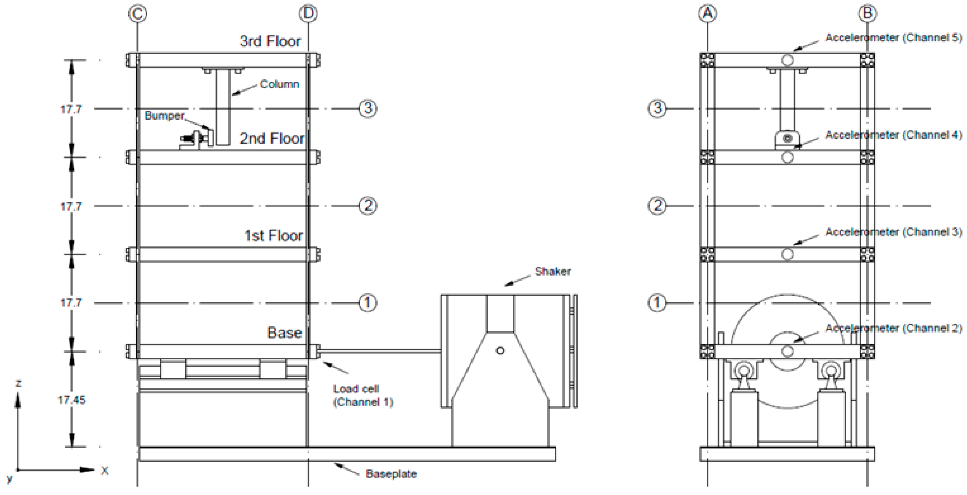This is due to the goal of this experimental setup being to mimic breathing crack behaviour [63]. A bumper–column bilinear mechanism achieves this: the column, hanging from the third floor, meets the bumper at the second story. This mechanism generates a directional nonlinear response, with stiffness increasing when the two are touching and pushing against each other. A scheme of the test structure is reported in Figure 8; the shaker and the four sensors’ locations are highlighted. A detailed description of the experimental setup and procedure is provided in [59]. The severity of the damage is modelled by moving closer or farther the column’s tip—when they are closer, the two elements come in touch for lower amplitudes of the driving force, thus causing major nonlinearities in the recorded response. The experimental THs have a total duration of 25.6 s, with $f_{s,exp}=320$ Hz. The dynamic input is a band-limited excitation (ranging 20–150 Hz), as defined in [3]. The 17 states (nine undamaged and eight damaged, with the first nine configurations being intended to emulate different operational and environmental conditions) were used for this investigation; they are summarized in

Table 6. Baseline, Undamaged and Damaged Scenarios for experimental validation.

Case	Description
1	Undamaged Baseline
2	Undamaged Added mass of 1.2 kg at the base
3	Undamaged Added mass of 1.2 kg at the 1st floor
4	Undamaged 87.5% stiffness reduction in one column of the 1st inter-story
5	Undamaged 87.5% stiffness reduction in two columns of the 1st inter-story
6	Undamaged 87.5% stiffness reduction in one column of the 2nd inter-story
7	Undamaged 87.5% stiffness reduction in one column of the 2nd inter-story
8	Undamaged 87.5% stiffness reduction in one column of the 3rd inter-story
9	Undamaged 87.5% stiffness reduction in two columns of the 3rd inter-story
10	Damaged Distance between bumper and column tip 0.20 mm
11	Damaged Distance between bumper and column tip 0.15 mm
12	Damaged Distance between bumper and column tip 0.13 mm
13	Damaged Distance between bumper and column tip 0.10 mm
14	Damaged Distance between bumper and column tip 0.05 mm
15	Damaged Bumper 0.20 mm from column tip, 1.2 kg added at the base
16	Damaged Bumper 0.20 mm from column tip, 1.2 kg added on the 1st floor
17	Damaged Bumper 0.10 mm from column tip, 1.2 kg added on the 1st floor

. All the output channels were used for the sensor setup considered. The test set was made up of 10 realisations for each scenario, totalling 180 simulated THs.

As for the second numerical case study, the definitions of ECO- and MO-MMFCCs have been changed to fit the structure of interest. For ECO-MMFCCs, the 90% bound of $f_{co}$ is approximately 78 Hz (averaging over the channels 3, 4, and 5 for the 50 realisations of Case 1); the $f_{s,exp}/2$ limit of LO-MMFCCs becomes 160 Hz. The array of the centre frequencies for MO-MMFCCs underwent some major rethinking. Being the structure basically assimilable to a three degrees-of-freedom oscillator (floor level does not count as it is subject to the input-induced rigid motion), only the first three frequencies have been retained. The remaining seven filters have been linearly spaced up to $f_s/2$, i.e., 160 Hz, thus resulting in

$$f_c=\left[31 54 71 83 96 109 122 135 148 160\right]$$

6. Results

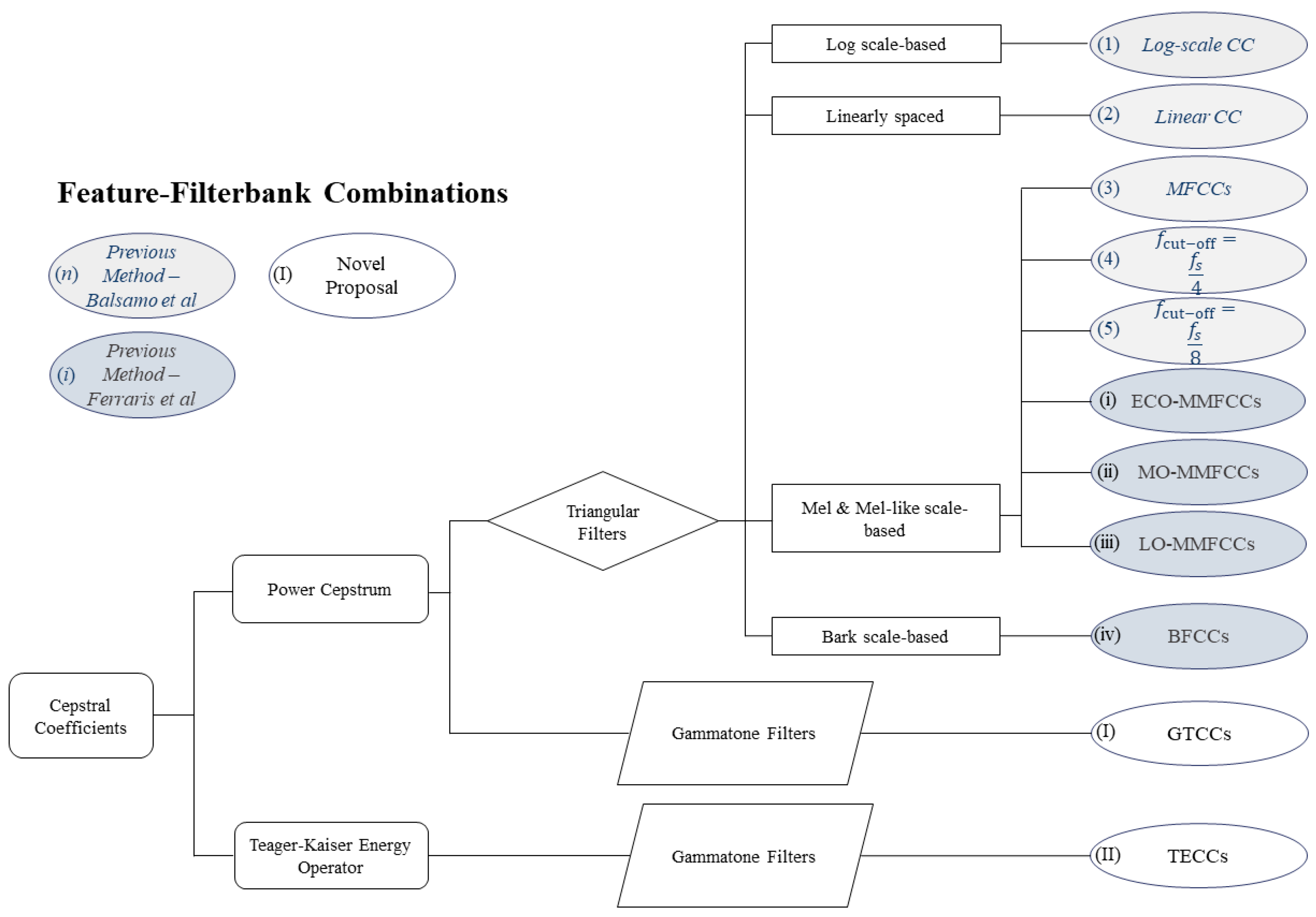
The results from previous works are reported for direct comparison. The methods applied are, by following the same nomenclature (see also Figure 2), (1) the log-scale CCs; (2) the linear CCs; (3) the classic definition of MFCCs; (4) the MFCCs with a cut-off frequency $f_{co}=\frac{f_s}{4}$; and, (5) the MFCCs with a cut-off frequency $f_{co}=\frac{f_s}{8}$ from [21]; the three proposed Mel-Modified Cepstral Coefficients (MMFCCs), i.e., the so-called (i) ECO-MMFCCs; (ii) MO-MMFCCs; and, (iii) LO-MMFCCs, from [22], plus the Bark-scale based (iv) BFCCs; finally, the novel features here presented, (I) the GTCCs and (II) the TECCs.

For better readability, this Section is split between the numerical and the experimental data. All the results are expressed in terms of type 1 (false positives, i.e., false alarms) and type 2 (false negatives or false acceptance) errors. In the latter case, the system is declared healthy while not being so; the opposite happens for false alarms. Being life-safety the main aim of any SHM procedure, type 1 errors are generally overlooked respect to their type 2 counterparts. Nevertheless, economical, practical, and psychological concerns make these as valuable as the other ones. A simple yet effective reasoning is that an alarm system constantly affected by false alarm will most probably be ignored when actual damage is effectively spotted. This nullifies any possible gain from the deployment of the SHM apparatus.

6.1. Results from the Numerical Simulations

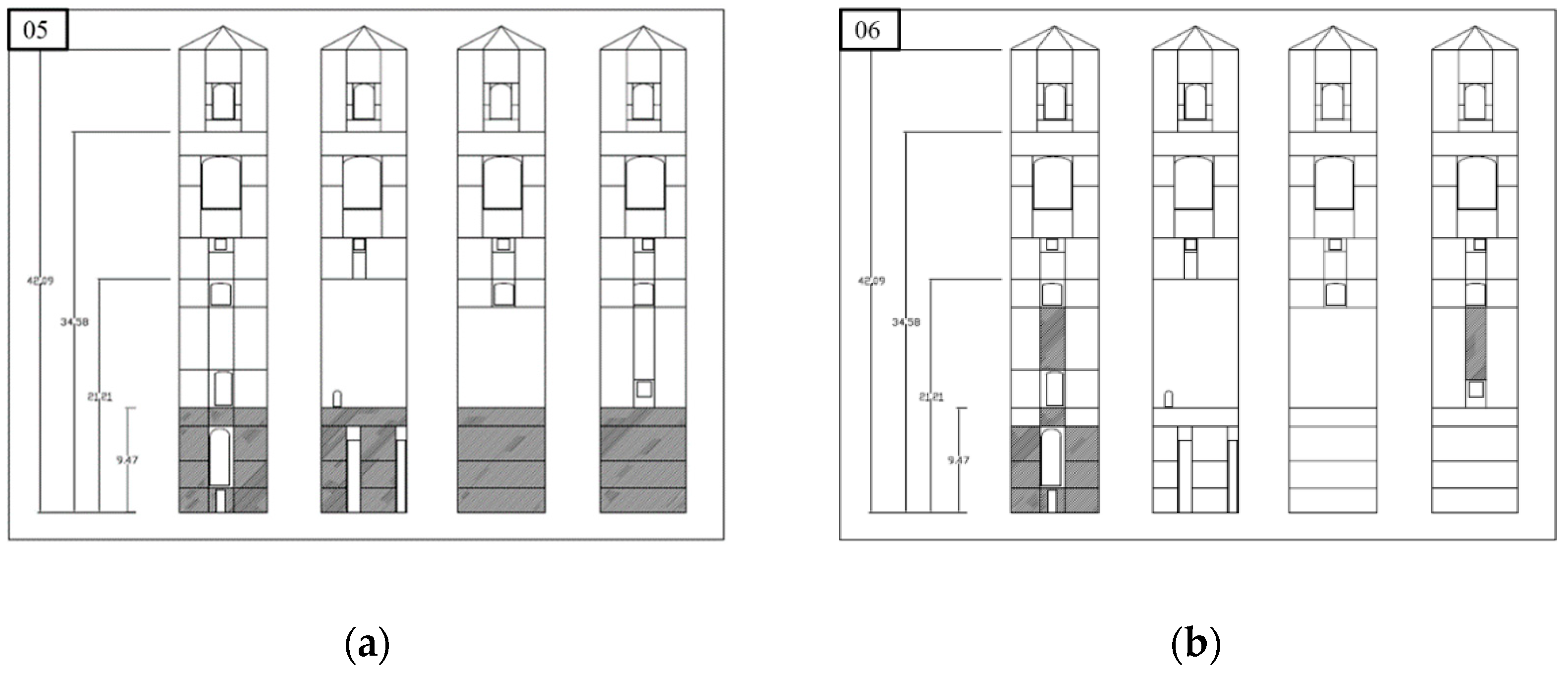
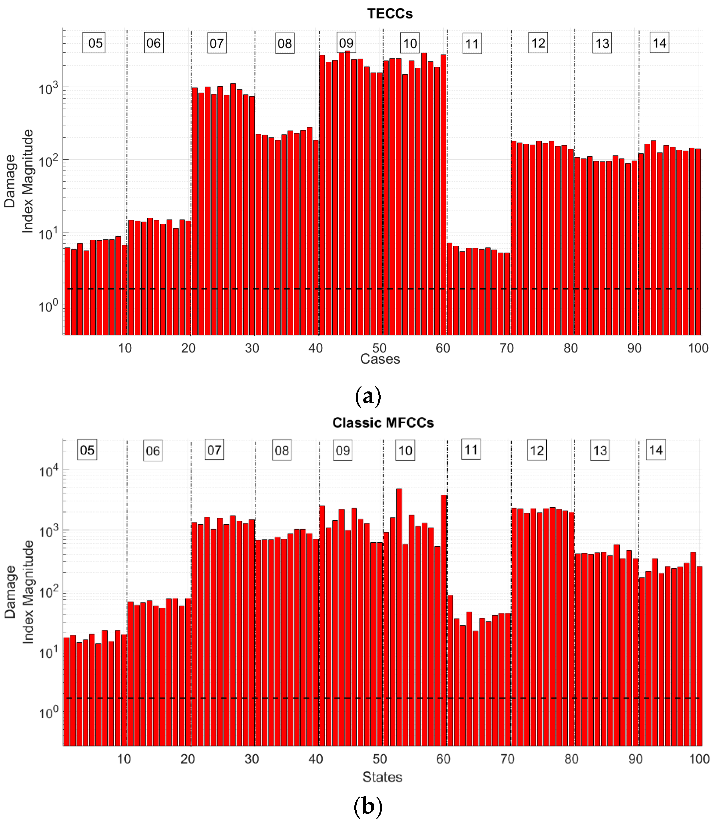
Regarding the first numerical case study (the Fossano bell tower), cases 00 to 04—i.e., the baseline and the story-uniform damage cases—are visually compared in Figure 9 to prove the algorithms capability to discern simpler configurations and widely extended damage from the normality model. Figure 10 shows the results for cases 05 to 10 (realistic damage scenarios). To estimate the robustness of each MFCC-based variant to false alarms, cases 15 to 18 (i.e., the scenarios with small fluctuations of the Young’s modulus respect to the baseline) are presented in Figure 11. Apart from the Teager-Kaiser Energy Cepstral Coefficients, the standard definition of MFCCs is also shown for comparison.

Table 7. Results for the first numerical case study (bell tower).

	Case 00	Cases 01–04	Cases 05–14	Cases 15–18
	Type 1 Errors [%]	Type 2 Errors [%]	Type 2 Errors [%]	Type 1 Errors [%]
MFCCs	60.00	0.00	0.00	45.00
$f_{\mathrm{cut}-\mathrm{off}}=\frac{1}{4} f_s$	30.00	0.00	0.00	45.00
$f_{\mathrm{cut}-\mathrm{off}}=\frac{1}{8} f_s$	30.00	0.00	0.00	45.00
Log-Scale	20.00	0.00	0.00	65.00
Linear	60.00	0.00	0.00	45.00
ECO-MMFCCs	20.00	0.00	0.00	62.50
MO-MMFCCs	10.00	0.00	0.00	62.50
LO-MMFCCs	20.00	0.00	0.00	65.00
BFCCs	60.00	0.00	0.00	47.50
GTCCs	20.00	0.00	0.00	60.00
TECCs	0.00	7.50	0.00	0.00

reports all results. In all figures, the black dashed line represents the defined threshold; bars exceeding it are coloured in red and they stand for the realisations labelled as damaged, while blue bars indicate values of DI under the prescribed threshold. From a statistical pattern recognition standpoint, this means that the cepstral features that correspond to that specific realisation have not departed considerably enough from their respective values for the reference baseline and are therefore labelled as undamaged.

As can be inferred from the first two columns of Table 7, the GTCCs, the Logarithmic Scale CCs, and the three Mel-Modified Scales (ECO-, MO-, and LO-MMFCCs) have all relatively low type 1 errors. The Damage Index values inside any given damage case are quite similar; that is a valuable proof of the robustness of the method. Bark-scale based CCs wrongly labelled as damaged 60% of the undamaged inputs coming from the same scenario used for the training. The TECCs were the most performing feature; in Figure 9.a one can clearly see that two out of the three mislabeled realisations for TECCs fall very short of the threshold. The third column in Table 7 (cases 05–14) shows that all algorithms work effectively in terms of damage detection. The classic definition of the Mel-Scale, the Bark-Scale, and the linear Scale nevertheless present some relatively larger fluctuations along the ten realisations of the same damage scenario with different inputs. The Log-Scale and the Mel-modified Scales provide more stable results, with a flat trend inside each damage scenario. This seems to indicate that a kind of nonlinear scale performs better than the constantly spaced filters. The filter shape might be even more incisive, as GTCCs and TECCs are all spaced according to the Bark Critical Bands yet perform better than triangular filters-based options both in terms of type I and II errors. Most of the algorithms recognise substantial gaps (Figure 8 and Figure 9) between different scenarios, which reflect the difference of damage extension; this seems to indicate a possibility to also exploit them for instances of damage severity assessment. Finally, the last column of Table 7 (cases 15 to 18) evidently portrays how only the TECCs correctly label all the proposed cases as unmodified respect to the baseline; the other features proved to be quite unsatisfactory, especially the Mel-Scale and Bark-Scale. That seems to once more validate the assumption that the straight application of the original definition of the mel-scale, tuned for speech processing aims, is not well-performing and proper corrections are needed. In particular, the scenarios with a variation in the material properties of ±0.25% are most often correctly labelled as healthy; otherwise, the ±1.00% deviation of the Young’s modulus provides DI values above the threshold. This phenomenon could be justified by the fact that even a relatively small difference between the pristine and modified mechanical properties of the model’s material cause a greater variation in the power spectrum of the structure, which is also reflected in the power and is wrongly seen as damage-induced. This aspect is not helpful in the damage detection process; the TKE operator seems to be more resilient to these slight changes. By summing up all of the damage scenarios of this first case, it turns out that of all features, the TECCs are the only one always correctly labelling the cases with realistic damage patterns (05–14) and the ones with global, small fluctuations of E, unrelated to damage (15–18). Indeed, the TECCs fall short of a perfect score for only three mislabeled realisations (out of 10) in case 01, which was also the most demanding scenario due to the proximity of the damage to the fixed end.

Table 8. Results for the second numerical case study (HAR wing).

	Cases 00–02	Cases 03–07
	Type 1 Errors [%]	Type 2 Errors [%]
MFCCs	66.67	0.00
$f_{\mathrm{cut}-\mathrm{off}}=\frac{1}{4} f_s$	66.67	0.00
$f_{\mathrm{cut}-\mathrm{off}}=\frac{1}{8} f_s$	66.67	0.00
Log-Scale	70.00	0.00
Linear	66.67	0.00
ECO-MMFCCs	66.67	0.00
MO-MMFCCs	66.67	0.00
LO-MMFCCs	66.67	0.00
BFCCs	66.67	0.00
GTCCs	66.67	0.00
TECCs	3.33	26.00 (*)

(*) 7.50% on Cases from 03 to 06.

reports the results for the second case study (the highly flexible prototype wing); Figure 12 graphically illustrates them. It can be inferred that, in this case, the exact detection of damage was more difficult. MFCCs and similar variants proved to be able to spot everywhere the damage but at the cost of not actually discerning it from the two cases with small perturbations. The TECCs, on the other hand, did not perform perfectly, yet they avoided all but one false alarm and were able to discern the damaged conditions decently in the inspected scenarios. If one does not take into account Case 07, which presents an imperceptible decrease of 0.03 Hz and went completely unnoticed by the trained algorithm, the type 2 error percentage drops to 7.50%, with two errors in Case 04, no one in Case 05, and a single mislabeled element in Case 06.

As in the previous case of the Fossano bell tower, this seems to point out the larger robustness of the TECCs feature to small changes, assumed here as statistical variations of the structural parameters and not directly linked to damage occurrence. A possible explanation comes from the TKE Operator being notably sensitive to frequency and amplitude changes, while much more robust than MFCCs to noise and minimal variations in the field of speech recognition accuracy.

6.2. Results from the Experimental Data

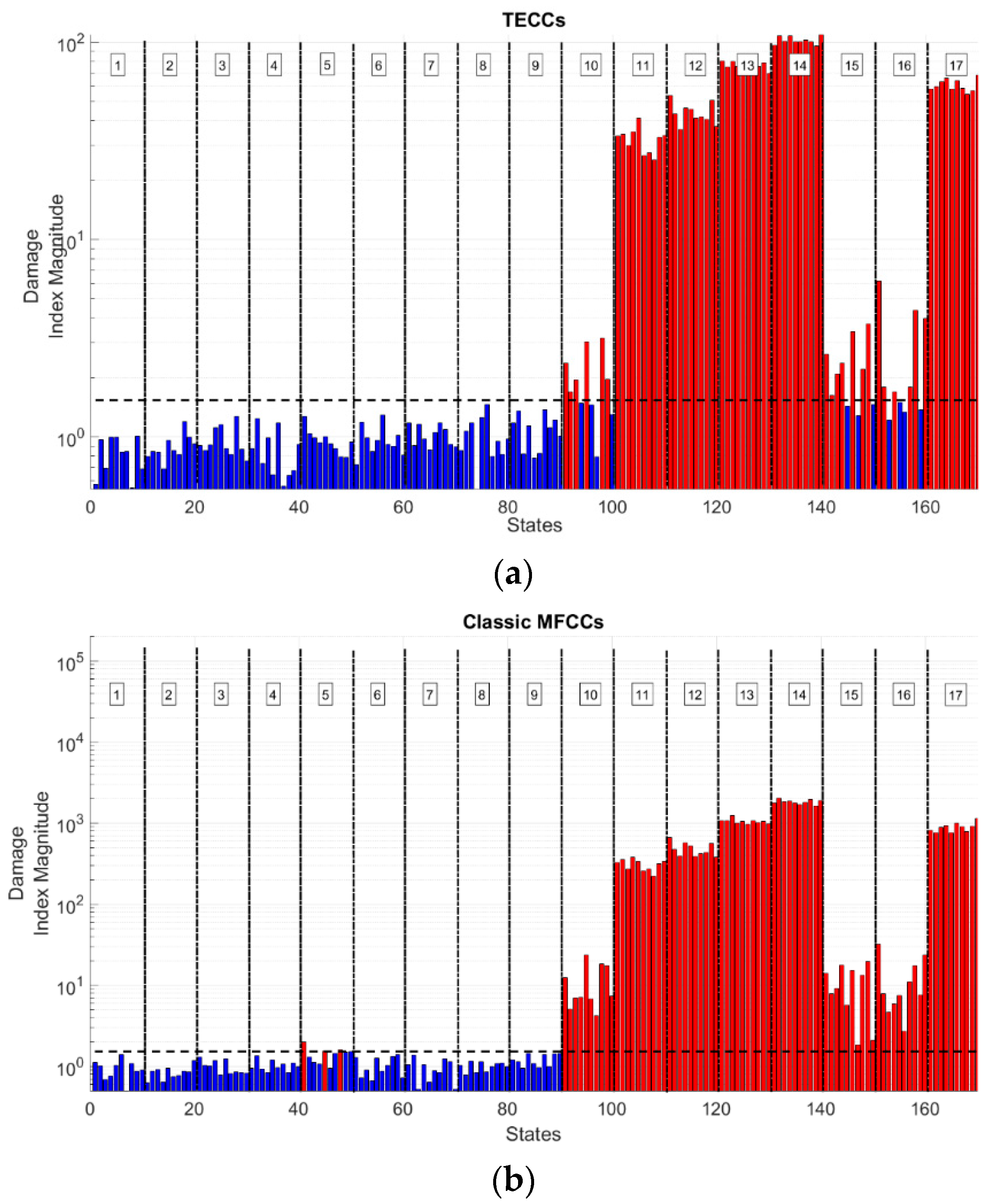
The results from experimental data are displayed here in Figure 13. As before, TECCs and classic MFCCs are only depicted due to space constraints.

Table 9. Results for the experimental case study.

	Cases 1–9	Cases 10–17
	Type 1 Errors [%]	Type 2 Errors [%]
MFCCs	3.33	0.00
$f_{\mathrm{cut}-\mathrm{off}}=\frac{1}{4} f_s$	5.56	0.00
$f_{\mathrm{cut}-\mathrm{off}}=\frac{1}{8} f_s$	7.78	1.25
Log-Scale	4.44	1.25
Linear	5.56	0.00
ECO-MMFCCs	4.44	0.00
MO-MMFCCs	2.22	22.50
LO-MMFCCs	12.22	25.00
BFCCs	3.33	0.00
GTCCs	4.44	0.00
TECCs	0.00	13.75

summarises the results, in terms of percentage of type 1 and 2 errors.

In interpreting the data, one must consider the different definition of ‘damage’ between the two numerical and the experimental case studies. The Fossano bell tower and the HAR prototype wing behave linearly in both damaged and pristine conditions; again, the difference between the two is only a matter of shifting natural frequencies. The experimental data have a completely different ‘meaning’ of damage, as here, differences in mass and stiffness are accounted as different operational conditions and the distinction between damaged and undamaged response lies solely on the presence of nonlinearities. In this latter case, the TECCs proved to be the only feature able to reach a 0% type 1 error in the test set, but only in spite of a relatively high type 2 error percentage, only surpassed by the recently proposed MO- and LO-MMFCCs. Nevertheless, a closer inspection of the several damaged and undamaged configurations allows for highlighting that this error is clustered in only three scenarios, respectively, cases 10, 15, and 16. Case 10 is the one with the slightest nonlinearity and, thus, is the most challenging to detect. The algorithm also struggled for cases 15 and 16, where changes in the frame’s mass are involved. On the other hand, all of the undamaged scenarios are recognised as such by means of the TECCs, while classic MFCCs generate some misclassifications for case 5 (which is the one with the largest stiffness reduction close to the base of the frame, where such structural changes have the most impact in the vibrational response).

Therefore, experimental results seem to validate what is expected from numerical simulations, that is to say: (i) a greater generalisation capability of the TECCs feature over closely-related alternatives; (ii) a strong robustness to false alarms but at the cost of some false negatives; and, (iii) a sensibility to shifts in the frequency content higher or at least comparable to MFCCs in its original form and proposed variants. On the other hand, the TECCs proved to be less sensitive to the presence of limited nonlinearities during changing operational conditions than to mass changes respect to the MFCCs and similar features; but this outcome might be specific of the experimental data utilised here.

6.2.1. Further Analysis of the Experimental Data

Some further tests were performed to better define the advantages of the proposed TECCs feature. For brevity sake, only the results for experimental data are reported; the same findings were observed for numerical data.

Firstly, the number and distribution of output channels were investigated. Four setups have been considered: setup #0, including all channels (numbered 2 to 5, see Figure 8), for which the results are already reported in Figure 13 and Table 9; setup #1 (channels 3, 4, and 5); setup #2 (channels 3 and 4); and finally, setup #3 (constituted by channels 4 and 5).

Table 10. Results according to the sensor setup considered.

	Sensor Setup #1		Sensor Setup #2		Sensor Setup #3
	Cases 1–9	Cases 10–17	Cases 1–9	Cases 10–17	Cases 1–9	Cases 10–17
	Type 1	Type 2	Type 1	Type 2	Type 1	Type 2
	Errors [%]	Errors [%]	Errors [%]	Errors [%]	Errors [%]	Errors [%]
MFCCs	4.44	0.00	2.22	1.25	2.22	0.00
$f_{\mathrm{cut}-\mathrm{off}}=\frac{1}{4} f_s$	3.33	0.00	1.11	0.00	1.11	0.00
$f_{\mathrm{cut}-\mathrm{off}}=\frac{1}{8} f_s$	5.56	0.00	3.33	1.25	3.33	0.00
Log-Scale	5.56	1.25	3.33	2.50	1.11	1.25
Linear	3.33	0.00	1.11	1.25	1.11	0.00
ECO-MMFCCs	3.33	0.00	1.11	0.00	1.11	0.00
MO-MMFCCs	2.22	25.00	3.33	30.00	1.11	27.50
LO-MMFCCs	10.00	25.00	0.00	23.75	2.22	25.00
BFCCs	1.11	0.00	0.00	2.50	1.11	0.00
GTCCs	2.22	0.00	2.22	1.25	2.22	1.25
TECCs	0.00	7.50	0.00	11.25	0.00	6.25
AR coefficients	13.33	0.00	12.22	0.00	6.67	0.00

enlists the results for these last three setups. Remarkably, this test evidenced what was already observed in [21], that is to say, MFCCs and similar features produce less accurate results when all of the acquisition channels are considered. This point was confirmed here for type 1 errors in two out of the three new setups considered. The same effects were encountered here for TECCs as well, with the same conditions: MFCCs systematically fail in labelling case 5 as undamaged, due to its relatively large shift in frequency, while TECCs struggle in classifying cases 10, 15, and 16 as damaged due to their lower level of nonlinear distortion.

Secondly, a comparison with a non-cepstral feature, the aforementioned AR coefficients, was also performed and reported in Table 10. The AIC approach was applied similarly to what done in [21]. An order of 12 was used for sensor setup #1 and #2; order 10 was applied instead for the sensor setup #3. It can be seen that the percentage of type 1 error is generally higher than most of the cepstral features that are proposed here.

The Central Processing Unit (CPU) time that was required for the training phase was then evaluated for all types of DSFs on non-optimised (yet comparable) versions of the code. This was tested by means of the Matlab^® stopwatch timer tic–toc;

Table 11. CPU time accordingly to the sensor setup considered (training phase).

	Sensor Setup #0	Sensor Setup #1	Sensor Setup #2	Sensor Setup #3
	CPU Time [s]	CPU Time [s]	CPU Time [s]	CPU Time [s]
MFCCs	1.60	1.31	1.00	1.03
$f_{\mathrm{cut}-\mathrm{off}}=\frac{1}{4} f_s$	1.63	1.31	1.01	1.03
$f_{\mathrm{cut}-\mathrm{off}}=\frac{1}{8} f_s$	1.62	1.35	1.04	1.04
Log-Scale	1.62	1.37	1.01	1.02
Linear	1.56	1.30	0.99	0.99
ECO-MMFCCs	1.56	1.31	1.00	1.02
MO-MMFCCs	1.58	1.29	1.00	0.99
LO-MMFCCs	1.59	1.29	1.01	0.99
BFCCs	1.58	1.32	1.02	1.00
GTCCs	1.78	1.38	1.06	1.07
TECCs	2.03	1.62	1.15	1.16

reports the results. One can clearly see that the computational time is comparable over the several sensor setups considered. Note that the timing accounts for training operations (feature extraction and population statistics estimation) and for threshold definition; the time required for data preprocessing, differently from what done in [21], was not considered, as it is identical for all features. This returns some faster results with respect to what is reported there. Moreover, the codes were run 10 times to avoid any computational variability; the average result is reported. As expected, the difference between MFCCs, similar variants, GTCCs and TECCs are minimal. It can be observed that GTCCs takes slightly longer than MFCCs (in the order of some fractions of a second), since there it is needed to build up the more complexly shaped gammatone filterbank. The TECCs require that additional time plus a bit more to compute the TKE operator out of the provided time arrays. In the case with all acquisition channels considered, these two operations make the code run in almost 30% more time (0.43 s on average). However, this delay is basically irrelevant if compared to the one that is needed to extract other features, such as the Auto-Regressive (AR) model coefficients [21].

Lastly, the standard deviation is proposed as a metric of dispersion for the results of the several realisations that belong to the same damage case, to quantitatively express the robustness of the classification.

Table 12. Standard deviation of Damage Index (DI) (sensor setup #0).

	σ(DI(n))-Cases 1 to 17
MFCCs	0.32, 0.20, 0.28, 0.19, 0.28, 0.32, 0.26, 0.21, 0.22, 6.21, 41.74, 62.64, 52.52, 72.21, 6.16, 8.63, 81.06.
Log-Scale	0.24, 0.29, 0.15, 0.22, 0.28, 0.22, 0.27, 0.22, 0.23, 3.29, 22.23, 33.42, 31.63, 32.26, 3.45, 5.39, 35.00.
Linear	0.29, 0.30, 0.22, 0.19, 0.27, 0.22, 0.24, 0.31, 0.24, 6.55, 39.27, 67.89, 46.22, 52.90, 5.50, 7.85, 72.59.
BFCCs	0.31, 0.20, 0.26, 0.19, 0.26, 0.35, 0.22, 0.21, 0.19, 6.73, 44.16, 68.87, 47.46, 64.38, 6.72, 9.36, 90.09.
GTCCs	0.20, 0.28, 0.15, 0.16, 0.20, 0.31, 0.32, 0.19, 0.24, 4.19, 25.88, 45.77, 51.07, 73.55, 3.80, 6.54, 41.64.
TECCs	0.18, 0.14, 0.17, 0.23, 0.14, 0.17, 0.13, 0.26, 0.22, 0.75, 4.78, 5.57, 4.25, 4.64, 0.84, 1.70, 4.35.

enlists the results for all 17 cases. Only the values for the sensor setup #0 and for MFCCs, log-scale CCs, linear CCs, BFCCs, GTCCs, and TECCs are reported here due to space constraints. The same behaviour was observed for the other setups as well. By considering ten realisations per investigated case, it can be observed that the use of TECCs as a DSF produce a much smaller scattering of the results, with the standard deviation never exceeding $\sigma =6$, while the same measure goes well over 50 or even 70 for MFCCs in some cases.

7. Conclusions

Any Structural Health Monitoring system relies on data, almost always pre-processed, and on features extrapolated from them. Mel-Frequency Cepstral Coefficients (MFCCs) have recently been proven to be effective in damage detection, relying on the cepstrum of the recorded structural response, even if margins for improvements were evident. The Teager-Kaiser Energy (TKE) operator has been proposed here as the basis for a similar feature, less subject to false positive mislabeling when used for Machine Learning. That is adherent to what is encountered for speech signals and well-known in the field of speaker and speech recognition. The investigation reported here spans over different structures, with different input and very different setups—varying acquisition parameters, such as the number of the output channels, the sampling frequency, and so on. Moreover, in the first and in the second numerical study, the damage was modelled as a linear reduction of stiffness inserted in a linear system, while the experimental case emulated the damage as a pointwise source of nonlinearity in an otherwise linear system and stiffness local reduction was intended as a change in the operational conditions that were unrelated to damage. This shows the excellent capability of generalisation of this approach.

The proposed damage sensitive feature, the Teager-Kaiser Energy Cepstral Coefficients (TECCs), has been benchmarked against the MFCCs and some similar variants. Interesting numerical and experimental results were achieved for both the linear and nonlinear models of damage.

The main conclusions are the following:

• the TECCs, MFCCs, and similar features perform efficiently both with damage emulated by a reduction of the Young’s modulus E or by the presence of nonlinearities, even if the signal is noisy;
• the Mel-Scale performed similarly to other nonlinear scales such as the Bark Scale or logarithmic spacing, with no clear best option among all the investigated case studies;
• the algorithms that resort to a Gammatone filterbank generally produced better results than the ones with triangular filters; even if the TECCs still outperforms the GTCCs;
• the TECCs present a strong reduction of the order of magnitude of the Damage Index (DI) with respect to MFCCs and similar options, in absolute terms; this does not affect the damage detection algorithm, as the relative distance between the ‘normality’ model and the damaged cases remains and seems even to increase;
• the Teager-Kaiser Energy Cepstral Coefficients outperforms all the competitors in terms of little or no type 1 errors, but it is slightly more prone to type 2 errors respect to MFCCs and derived features;
• with respect to non-cepstral features, such as the AR coefficients, the main benefits lie in the less computational cost and greater robustness to noise and to confounding influences, such as environmental and operational effects, unrelated to damage.

The outcomes of this research leave plenty of room for improvements. Indeed, apart from the TECCs and other cepstral-based alternatives, wavelet-based alternatives are of great interest. The Mel-Frequency Discrete Wavelet Coefficients may be a relevant alternative. Thanks to the Discrete Wavelet Transform, the filter spacing issue is by-passed; filter shaping is reduced to the selection of the mother wavelet. The Authors are committed to pursuing further studies in this direction.

References

1. Farrar, C.R.; Worden, K. Structural Health Monitoring: A Machine Learning Perspective; John Wiley & Sons: Hoboken, NJ, USA, 2013. [Google Scholar]
2. Doebling, S.W.; Farrar, C.R.; Prime, M.B. A Summary Review of Vibration-Based Damage Identification Methods. Shock Vib. Dig. 1998, 30, 91–105. [Google Scholar] [CrossRef]
3. Figueiredo, E.; Park, G.; Farrar, C.R.; Worden, K.; Figueiras, J. Machine learning algorithms for damage detection under operational and environmental variability. Struct. Health Monit. 2011, 10, 559–572. [Google Scholar] [CrossRef]
4. Sohn, H.; Farrar, C.R.; Hunter, N.F.; Worden, K. Structural Health Monitoring Using Statistical Pattern Recognition Techniques. J. Dyn. Syst. Meas. Control 2001, 123, 706–711. [Google Scholar] [CrossRef]
5. Amezquita-Sanchez, J.P.; Adeli, H. Signal Processing Techniques for Vibration-Based Health Monitoring of Smart Structures. Arch. Comput. Methods Eng. 2016, 23, 1–15. [Google Scholar] [CrossRef]
6. Bonato, P.; Ceravolo, R.; Stefano, A. De Time-Frequency and Ambiguity Function Approaches in Structural Identification. J. Eng. Mech. 1997, 123, 1260–1267. [Google Scholar] [CrossRef]
7. Bonato, P.; Ceravolo, R.; De Stefano, A.; Molinari, F. Cross-Time Frequency Techniques for the Identification of Masonry Buildings. Mech. Syst. Signal Process. 2000, 14, 91–109. [Google Scholar] [CrossRef]
8. Law, S.S.; Zhu, X.Q.; Tian, Y.J.; Li, X.Y.; Wu, S.Q. Statistical damage classification method based on wavelet packet analysis. Struct. Eng. Mech. 2013, 46, 459–486. [Google Scholar] [CrossRef]
9. Liu, J.; Wang, Z.; Liu, J.-L.; Wang, Z.-C.; Ren, W.-X.; Li, X.-X. Structural time-varying damage detection using synchrosqueezing wavelet transform. Smart Struct. Syst. 2015, 15, 1738–1991. [Google Scholar] [CrossRef]
10. Wang, C.; Ren, W.X.; Wang, Z.C.; Zhu, H.P. Time-varying physical parameter identification of shear type structures based on discrete wavelet transform. Smart Struct. Syst. 2014, 14, 831–845. [Google Scholar] [CrossRef]
11. Pnevmatikos, N.; Blachowski, B.D.; Hatzigeorgiou, G.; Pnevmatikos, N.G.; Blachowski, B.; Hatzigeorgiou, G.D.; Swiercz, A. Wavelet analysis based damage localization in steel frames with bolted connections. Smart Struct. Syst. 2016, 18, 1738–1991. [Google Scholar] [CrossRef]
12. Civera, M.; Zanotti Fragonara, L.; Surace, C. Nonlinear Dynamics of Cracked, Cantilevered Beam-like Structures Undergoing Large Deflections. In Proceedings of the 2019 IEEE 5th International Workshop on Metrology for AeroSpace (MetroAeroSpace), Torino, Italy, 19–21 June 2019. [Google Scholar]
13. Pines, D.; Salvino, L. Structural health monitoring using empirical mode decomposition and the Hilbert phase. J. Sound Vib. 2006, 294, 97–124. [Google Scholar] [CrossRef]
14. Civera, M.; Filosi, C.M.; Pugno, N.M.; Silvestrini, M.; Surace, C.; Worden, K. Assessment of vocal cord nodules: A case study in speech processing by using Hilbert-Huang Transform. J. Phys. Conf. Ser. 2017, 842, 012025. [Google Scholar] [CrossRef]
15. Childers, D.G.; Skinner, D.P.; Kemerait, R.C. The cepstrum: A guide to processing. Proc. IEEE 1977, 65, 1428–1443. [Google Scholar] [CrossRef]
16. Zheng, H.; Mita, A. Damage indicator defined as the distance between ARMA models for structural health monitoring. Struct. Control Health Monit. 2008, 15, 992–1005. [Google Scholar] [CrossRef]
17. Kim, J.T.; Lyon, R.H. Cepstral analysis as a tool for robust processing, deverberation and detection of transients. Mech. Syst. Signal Process. 1992, 6, 1–15. [Google Scholar] [CrossRef]
18. Peeters, C.; Guillaume, P.; Helsen, J. A comparison of cepstral editing methods as signal pre-processing techniques for vibration-based bearing fault detection. Mech. Syst. Signal Process. 2017, 91, 354–381. [Google Scholar] [CrossRef]
19. Randall, R.B. A History of Cepstrum Analysis and its Application to Mechanical Problems. Mech. Syst. Signal Process. 2017, 97, 3–19. [Google Scholar] [CrossRef]
20. Balsamo, L.; Betti, R.; Beigi, H. Structural Damage Detection Using Speaker Recognition Techniques. In Proceedings of the 11th International Conference on Structureal Safety and Reliability (ICOSSAR), New York, NY, USA, 16–20 June 2013. [Google Scholar]
21. Balsamo, L.; Betti, R.; Beigi, H. A structural health monitoring strategy using cepstral features. J. Sound Vib. 2014, 333, 4526–4542. [Google Scholar] [CrossRef]
22. Ferraris, M.; Civera, M.; Ceravolo, R.; Surace, C.; Betti, R. Using Enhanced Cepstral Analysis for Structural Health Monitoring; Springer: Singapore, 2020; pp. 150–165. [Google Scholar]
23. Dimitriadis, D.; Maragos, P.; Potamianos, A. Auditory Teager Energy Cepstrum Coefficients for Robust Speech Recognition. In Proceedings of the 9th European Conference on Speech Communication and Technology, Lisbon, Portugal, 4–8 September 2005. [Google Scholar]
24. Kaiser, J.F. On a simple algorithm to calculate the “energy” of a signal. In Proceedings of the International Conference on Acoustics, Speech, and Signal Processing, Albuquerque, NM, USA, 3–6 April 1990; pp. 381–384. [Google Scholar]
25. Schluter, R.; Bezrukov, I.; Wagner, H.; Ney, H. Gammatone Features and Feature Combination for Large Vocabulary Speech Recognition. In Proceedings of the 2007 IEEE International Conference on Acoustics, Speech and Signal Processing—ICASSP ’07, Honolulu, HI, USA, 15–20 April 2007; pp. 649–652. [Google Scholar]
26. Vakman, D. On the analytic signal, the Teager-Kaiser energy algorithm, and other methods for defining amplitude and frequency. IEEE Trans. Signal Process. 1996, 44, 791–797. [Google Scholar] [CrossRef]
27. Tran, V.T.; AlThobiani, F.; Ball, A. An approach to fault diagnosis of reciprocating compressor valves using Teager—Kaiser energy operator and deep belief networks. Expert Syst. Appl. 2014, 41, 4113–4122. [Google Scholar] [CrossRef]
28. Henríquez Rodríguez, P.; Alonso, J.B.; Ferrer, M.A.; Travieso, C.M. Application of the Teager-Kaiser energy operator in bearing fault diagnosis. ISA Trans. 2013, 52, 278–284. [Google Scholar] [CrossRef]
29. Ceravolo, R.; Pistone, G.; Fragonara, L.Z.; Massetto, S.; Abbiati, G. Vibration-Based Monitoring and Diagnosis of Cultural Heritage: A Methodological Discussion in Three Examples. Int. J. Archit. Herit. 2016, 10, 375–395. [Google Scholar] [CrossRef]
30. Carpinteri, A.; Lacidogna, G. Damage monitoring of an historical masonry building by the acoustic emission technique. Mater. Struct. 2006, 39, 161–167. [Google Scholar] [CrossRef]
31. Carpinteri, A.; Lacidogna, G. Structural Monitoring and Integrity Assessment of Medieval Towers. J. Struct. Eng. 2006, 132, 1681–1690. [Google Scholar] [CrossRef]
32. Carpinteri, A.; Invernizzi, S.; Lacidogna, G. In situ damage assessment and nonlinear modelling of a historical masonry tower. Eng. Struct. 2005, 27, 387–395. [Google Scholar] [CrossRef]
33. Pontillo, A.; Hayes, D.; Dussart, G.X.; Lopez Matos, G.E.; Carrizales, M.A.; Yusuf, S.Y.; Lone, M.M. Flexible High Aspect Ratio Wing: Low Cost Experimental Model and Computational Framework. In Proceedings of the 2018 AIAA Atmospheric Flight Mechanics Conference, Reston, VA, USA, 8–12 January 2018. [Google Scholar]
34. Lanzoni, L.; Tarantino, A.M. Equilibrium configurations and stability of a damaged body under uniaxial tractions. Z. Angew. Math. Phys. 2014, 66, 171–190. [Google Scholar] [CrossRef]
35. Tarantino, A.M. Equilibrium paths of a hyperelastic body under progressive damage. J. Elast. 2014, 114, 225–250. [Google Scholar] [CrossRef]
36. Bedon, C. Diagnostic analysis and dynamic identification of a glass suspension footbridge via on-site vibration experiments and FE numerical modelling. Compos. Struct. 2019, 216, 366–378. [Google Scholar] [CrossRef]
37. Bogert, B.P. The quefrency alanysis of time series for echoes; Cepstrum, pseudo-autocovariance, cross-cepstrum and saphe cracking. Time Ser. Anal. 1963, 09–243. [Google Scholar]
38. Stevens, S.S.; Volkmann, J.; Newman, E.B. A Scale for the Measurement of the Psychological Magnitude Pitch. J. Acoust. Soc. Am. 1937, 8, 185–190. [Google Scholar] [CrossRef]
39. Satyam, M.; Sudhakara, R.; Devy, C.G. Cepstrum Analysis: An Advanced Technique in Vibration Analysis of Defects in Rotating Machinery. Def. Sci. J. 1994, 44, 53–60. [Google Scholar] [CrossRef]
40. Noll, A.M. Cepstrum Pitch Determination. J. Acoust. Soc. Am. 1967, 41, 293–309. [Google Scholar] [CrossRef] [PubMed]
41. De Krom, G. A Cepstrum-Based Technique for Determining a Harmonics-to-Noise Ratio in Speech Signals. J. Speech Lang. Hear. Res. 1993, 36, 254–266. [Google Scholar] [CrossRef] [PubMed]
42. Oppenheim, A.V.; Schafer, R.W.; Buck, J.R. Discrete-Time Signal Processing; Prentice Hall: Upper Saddle River, NJ, USA, 1999; ISBN 0130834432. [Google Scholar]
43. Beigi, H. Fundamentals of Speaker Recognition; Springer: Berlin/Heidelberg, Germany, 2016; ISBN 9781489979223. [Google Scholar]
44. Mermelstein, P. Distance measures for speech recognition, psychological and instrumental. Pattern Recognit. Artif. Intell. 1976, 116, 374–388. [Google Scholar]
45. Bridle, J.S.; Brown, M.D.; Chamberlain, R.M. An experimental automatic word recognition system; Technical Report JSRU No. 1003; Joint Speech Research Unit: Ruislip, England, 1974. [Google Scholar]
46. Stevens, S.S.; Volkmann, J. The Relation of Pitch to Frequency: A Revised Scale. Am. J. Psychol. 1940, 53, 329–353. [Google Scholar] [CrossRef]
47. Hermansky, H.; Morgan, N.; Hirsch, H.-G. Recognition of speech in additive and convolutional noise based on RASTA spectral processing. In Proceedings of the IEEE International Conference on Acoustics Speech and Signal Processing, Minneapolis, MN, USA, 27–30 April 1993; Volume 2, pp. 83–86. [Google Scholar]
48. Fant, G. Acoustic Theory of Speech Production: With Calculations Based on X-ray Studies of Russian Articulations; Mouton: The Hague, Netherlands, 1970; ISBN 9027916004. [Google Scholar]
49. Umesh, S.; Cohen, L.; Nelson, D. Fitting the Mel Scale. In Proceedings of the 1999 IEEE International Conference on Acoustics, Speech, and Signal Processing, Phoenix, AZ, USA, 15–19 March 1999. [Google Scholar]
50. Zwicker, E. Subdivision of the Audible Frequency Range into Critical Bands (Frequenzgruppen). J. Acoust. Soc. Am. 1961, 33, 248. [Google Scholar] [CrossRef]
51. Irino, T.; Patterson, R.D. A time-domain, level-dependent auditory filter: The gammachirp. J. Acoust. Soc. Am. 1997, 101, 412–419. [Google Scholar] [CrossRef]
52. Traunmüller, H. Analytical expressions for the tonotopic sensory scale. J. Acoust. Soc. Am. 1990, 88, 97–100. [Google Scholar] [CrossRef]
53. Moore, B.C.J.; Glasberg, B.R. Suggested formulae for calculating auditory-filter bandwidths and excitation patterns. J. Acoust. Soc. Am. 1983, 74, 750–753. [Google Scholar] [CrossRef]
54. Herrera, A.; Del Rio, F. Frequency bark cepstral coefficients extraction for speech analysis by synthesis. J. Acoust. Soc. Am. 2010, 128, 2290. [Google Scholar] [CrossRef]
55. Slaney, M. An Efficient Implementation of the Patterson-Holdsworth Auditory Filter Bank; Technical Report Apple Computer No. 35, Perception Group—Advanced Technology Group, Cupertino, California (USA). 1993. Available online: https://engineering.purdue.edu/~malcolm/apple/tr35/PattersonsEar.pdf (accessed on 21 November 2019).
56. Teager, H.M.; Teager, S.M. Evidence for Nonlinear Sound Production Mechanisms in the Vocal Tract. In Speech Production and Speech Modelling; Springer: Dordrecht, The Netherlands, 1990; pp. 241–261. [Google Scholar]
57. Maragos, P.; Kaiser, J.F.; Quatieri, T.F. On amplitude and frequency demodulation using energy operators. IEEE Trans. Signal Process. 1993, 41, 1532–1550. [Google Scholar] [CrossRef]
58. Skowronski, M.D.; Harris, J.G. Increased mfcc filter bandwidth for noise-robust phoneme recognition. In Proceedings of the IEEE International Conference on Acoustics Speech and Signal Processing, Orlando, FL, USA, 13–17 May 2002; pp. 801–804. [Google Scholar]
59. Figueiredo, E.; Park, G.; Figueiras, J. Structural Health Monitoring Algorithm Comparisons Using Standard Data Sets; Los Alamos National Lab.(LANL): Los Alamos, NM, USA, 2009. [Google Scholar]
60. Ververidis, D.; Kotropoulos, C. Information Loss of the Mahalanobis Distance in High Dimensions: Application to Feature Selection. IEEE Trans. Pattern Anal. Mach. Intell. 2009, 31, 2275–2281. [Google Scholar] [CrossRef] [PubMed]
61. Civera, M.; Zanotti Fragonara, L.; Surace, C. Video Processing Techniques for the Contactless Investigation of Large Oscillations. J. Phys. Conf. Ser. 2019, 1249, 012004. [Google Scholar] [CrossRef]
62. Civera, M.; Zanotti Fragonara, L.; Surace, C.; Civera, M.; Zanotti Fragonara, L.; Surace, C. Using Video Processing for the Full-Field Identification of Backbone Curves in Case of Large Vibrations. Sensors 2019, 19, 2345. [Google Scholar] [CrossRef] [PubMed] [Green Version]
63. Bovsunovsky, A.; Surace, C. Non-linearities in the vibrations of elastic structures with a closing crack: A state of the art review. Mech. Syst. Signal Process. 2015, 62–63, 129–148. [Google Scholar] [CrossRef]
Figure 1. The Mel-Frequency Cepstral Coefficients (MFCCs) extraction procedure; frame #5 is used as an example. From left to right: the acceleration time history and its corresponding power spectrum, the power cepstrum of the same, and the resulting MFCCs in the quefrency domain.
Applsci 09 05064 g001
Figure 2. Conceptual relationships between the proposed methodology and the other tested approaches.
Applsci 09 05064 g002
Figure 3. Flowchart of the Teager-Kaiser Energy Cepstral Coefficients (TECCs) extraction procedure.
Applsci 09 05064 g003
Figure 4. Structural scheme of the bell tower (to the right in the image) and picture of its front view (to the left); autofrettage interventions are clearly visible on the external façades.
Applsci 09 05064 g004
Figure 5. Left: scheme of the sensor placement and direction of the acquisition channels (red, green, and yellow arrows). Right: the updated Finite Element (FE) model.
Applsci 09 05064 g005
Figure 6. (a) to (f): Damage Scenarios 05–10, in the same order. The scenarios have been derived by observation of similar structures damaged by earthquakes; areas with reduced Young’s Modulus are portrayed in grey.
Applsci 09 05064 g006aApplsci 09 05064 g006b
Figure 7. (a) Areas subject to decreased Young’s modulus (b) Damage scenarios.
Applsci 09 05064 g007
Figure 8. The experimental test setup schematics.
Applsci 09 05064 g008
Figure 9. Damage indexes for TECCs (a) and MFCCs (b); first numerical case study (Fossano bell tower), scenarios 00–04 (story-level damage).
Applsci 09 05064 g009
Figure 10. Damage indexes for TECCs (a) and MFCCs (b); first numerical case study (Fossano bell tower), scenarios 05–14 (realistic damage).
Applsci 09 05064 g010
Figure 11. Damage indexes for TECCs (a) and MFCCs (b); first numerical case study (Fossano bell tower), scenarios 15–18 (no damage).
Applsci 09 05064 g011aApplsci 09 05064 g011b
Figure 12. Damage indexes for TECCs (a) and MFCCs (b); second numerical case study (highly flexible prototype wing).
Applsci 09 05064 g012
Figure 13. Damage indexes for TECCs (a) and MFCCs (b); and, experimental data.
Applsci 09 05064 g013