Report on a Plus-Energy District with Low-Temperature DHC Network, Novel Agrothermal Heat Source, and Applied Demand Response

Abstract

District heating and cooling networks can pose the possibility of including a variety of renewable energy sources as well as waste heat into a district’s heat supply concept. Unfortunately, low demand densities as they increasingly occur through higher building energy standards and in rural areas render conventional heating and cooling networks inefficient. At the same time, power-to-heat is becoming more and more important to make use of a larger amount of renewable energy sources on the electrical side by providing more flexibility by means of demand response and demand-side management. Within this work, a rural Plus-Energy settlement is presented addressing those topics by a low-temperature district heating and cooling network connected to a novel agrothermal collector supplying 23 residential buildings with decentralized heat pumps and PV systems. The collector, the network, and six of the buildings are equipped with comprehensive monitoring equipment. Within those buildings, forecast and optimization algorithms are implemented to adapt their heat pump operation to enable an increase of self-consumption, to include flexible electricity tariffs, and also to participate in power markets. Thereby, for the low-temperature district heating and cooling network, it has been shown that the concept can operate in the future at competitive heat costs. On the building level, up to 50% of cost savings could be achieved under ideal conditions with the optimization of the self-consumption of PV electricity. However, to ensure optimal results, the individual system components have to be dimensioned for this task.

1. Introduction

The expansion of wind power and photovoltaics is progressing inexorably. Due to that, renewable heat supply has often received less attention in the past. At the same time, in many countries, the private households contribute to the high energy consumption, especially the heat consumption. Here, DHC (district heating and cooling) networks can offer several benefits compared to decentralized heating systems such as higher heating plant efficiencies, cogeneration, and tapping waste heat potentials. Unfortunately, first to fourth generation DHC networks cause many heat losses due to the distribution process, the high temperature levels (above 70–200 °C) and often weak insulation (first to third generation) [1]. Therefore, they also require a high demand density to operate economically, making them little or not applicable in rural areas. Future construction of more “climate neutral” buildings and the ongoing refurbishment of existing buildings will reduce the demand for conventional district heating grids even more, resulting in a reduced heating demand density also in more dense areas [2]. Furthermore, in densely populated areas, district heating is often more expensive compared to conventional, mainly fossil fuel-based decentralized heat supply systems [3]. Reducing the grid temperature in fifth generation DHC networks can reduce both grid losses and construction costs for insulation [4], and thus lead to competitive specific heating prices in less dense areas. Low temperature heating and cooling sources such as vertical heat exchangers, low-temperature waste heat, or horizontal ground collectors can supply these fifth generation low-temperature DHC networks [5]. With temperature levels of the distribution network around the soil temperature, heat losses can be equalized [6]. In some cases, the fluid temperature is even below the soil temperature, which generates a heat yield along the length of the piping [6]. De facto, the distribution network serves as a horizontal heat collector.

Nowadays, especially in Germany, a lot of research is carried out in the field of low-temperature DHC, as displayed in

Table 1. Summary of current research projects in Germany developing low-temperature district heating and cooling (DHC) networks with geothermal energy sources.

Project Name	Reference Number	Timespan	Short Summary
BestHeatNet	03ET1626A	12.2018–10.2023	Practical development and testing of a low-temperature DHC network with variable renewable energy sources
Envisage Plus	03ET1465A	01.2017–03.2021	Low-temperature DHC network with agrothermal collector
ErdEis	03ET1382A	09.2016–03.2019	Utilization of latent heat and geothermal heat storage for the districts
ErdEisII	03ET1634A	03.2019–02.2022	Low-temperature DHC network with a frozen soil storage system
Grubenwasser in Bochum-Werne	0327400Z	10.2011–19.2016	Use of heat from mine water for a low-temperature DHC network
Kassel Zum Feldlager	03ET1336A	11.2015–08.2019	New build district in Kassel (Germany) with solar thermal and vertical geothermal systems as the heat supply
Living Lab Energy Campus	03ET1551A	01.2018–12.2020	Field site to test a self-sufficient area network with renewable energy sources
LowExTra	03ET1237A	07.2014–12.2017	Low-temperature DHC network for the integration of multiple renewable energy sources (solar, thermal, geothermal)
NATAR	03ET1425A	01.2017–09.2020	Low-temperature DHC network to provide regulatory power
Neckarpark Stuttgart	03ET1156A	05.2013–04.2020	Low-temperature DHC network fed by sewage out of the sewer

.

Within those projects, the municipality of Wüstenrot, which is addressed in this work, was one of the first cities trying horizontal heat exchangers together with a low-temperature DHC network for research purposes in 2011. Since then, the development of the systems is progressing. In the summer of 2019, the local energy distributor of Bad Nauheim (Germany) built the largest known horizontal geothermal collector with 22,000 m² of collector surface distributed over two layers [7,8]. Together with the approximately 6 km long low-temperature district heating and cooling network, the system supplies heat and cooling for around 1000 people in more than 400 residential units.

A wider range of different technologies and national differences is addressed by the European funded research project called “REWARDHeat—Renewable and Waste Heat Recovery for Competitive District Heating and Cooling”, which focuses on demonstrating low-temperature DHC networks and their business models. Twenty-eight partners around Europe use their knowledge of low-temperature DHC to make it even more competitive. The project is coordinated by EURAC (the European academy of Bozen / Bolzano). The knowledge gained from the Plus-Energy settlement “Wüstenrot” will be also considered in the project.

Decentralized brine/water heat pumps complement low-temperature DHC networks ideally. Low-temperature DHC networks and heat pump systems can be used for sector coupling—a very promising approach [9]. This is relevant, as the current situation in Germany points toward that in 2018, the share of RES (renewable energy sources) within the entire consumed electricity was at approximately 40% [9], but the share of RES within the consumed heat was approximately 14% [10]. The transfer of excess electricity can serve as heating (power-to-heat), but it also allows direct grid-stabilizing measures. For instance, it can counteract the increasing challenge that the share of RES in the (German) electricity grid poses due to its high volatility. Power-to-heat applications based on heat pumps show a promising and largely untapped potential as they could provide a DR (demand response) potential of up to 20 GW_el in the year 2030 [11]. Together with DR, DSM (demand-side management) can play an important role to ensure future power grid stability [12]. In addition, technologies such as battery storage, regulatory measures such as strategic stability reserve plants, or innovative incentives in the private sector such as flexible end-user electricity tariffs can provide solutions for this demanding task [13,14]. Advanced prediction, optimization, and control algorithms are needed to implement DR and DSM in HVAC (heating, ventilation, and air-conditioning) and in specific within-heat pump systems, as well as to increase the system efficiency.

This work focuses on the Plus-Energy settlement in Wüstenrot, its novel agrothermal heat source combined with a low-temperature DHC network, and 23 residential buildings that are connected to the grid. All buildings have high-energy efficiency standards, are equipped with decentralized heat pumps, PV (photovoltaic) systems, some with battery storages and all relevant electrical and thermal energy flows are monitored in detail. At first, a comprehensive overview is given about the Plus-Energy settlement, including its planning, realization, and construction (costs). Monitored results of the settlement’s heat demand and of the novel agrothermal collector system and its operational characteristics are presented. Further, the PV and heat pump concept as well as the approach on economical assessment are explained. Then, the focus is taken to the building level where currently work is still in progress regarding optimized building operation. Thereby, strategies for the application of DR and DSM are presented. The utilization of white box and self-learning black box simulation models for the prediction and application of evolutionary (genetic) algorithms for optimization are explained, and a validation together with an estimation of the prediction inaccuracy is carried out. Based on the knowledge gained and on the models developed, results of the ongoing work are presented, including an assessment of the agrothermal low-temperature DHC systems costs, the building-side end-user costs, results for the optimization parameters, as well as simulation-based estimations on self-consumption, flexible electricity tariffs, and power markets.

2. The Wüstenrot Pilot Site

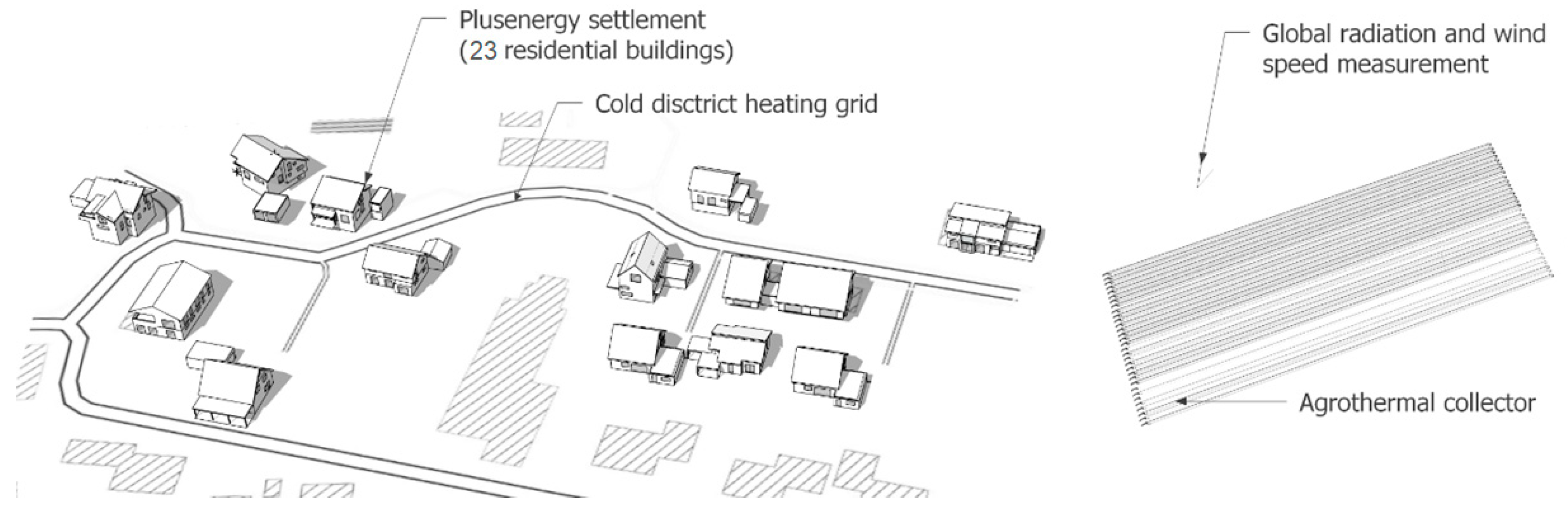
The Plus-Energy settlement “Vordere Viehweide” (see Figure 1) consists of 23 recently built residential buildings with high-energy standards. All buildings are equipped with decentralized heat pumps, thermal buffer storages, PV systems between 6 and 13 kW_p, and in some cases with battery storages. All heat pumps are connected to a low-temperature DHC network. A novel large-scale, very shallow horizontal geothermal collector also called an “agrothermal collector” works as the heating and cooling source. The name “agrothermal collector” defines the simultaneous use of very shallow geothermal energy from the soil together with agricultural usability on top of the surface.

The settlement was originally planned within the national research project “EnVisaGe” [15] in Wüstenrot, Germany. There, it was part of a larger strategy for the whole municipality of Wüstenrot with the aim to produce more thermal and electrical energy by its annual balance than its demand to become energy independent. Investigations showed that this was reasonable on the electricity side, but not on the thermal side, underlining the importance of sector coupling. Further information is described in the final report of the specific project [16].

Within the research projects EnVisaGe, Envisage Plus [17], and the Horizon2020 project Sim4Blocks [18], a settlement monitoring was installed in 11 out of 23 buildings. The monitoring of six buildings is more detailed, comprising all thermal and electrical energy flows together with the temperatures in detail (intensive monitoring). By doing so, it is possible to make a statement of the buildings’ performance. The other five buildings’ monitoring includes as well thermal and electrical monitoring. However, here the energy flows are measured at the buildings’ boundaries (extensive monitoring). All monitoring data are accessible via a cloud-based monitoring and control system. The pilot site also contributed to work in the Horizon 2020 projects FLEXYNETS [19] and REFLEX [20]. The results of the innovative low-temperature DHC system together with the agrothermal use are supporting the energy transition in Germany.

2.1. Planning, Realization, and Construction Costs

At the beginning, it was planned to connect 25 buildings to the low-temperature DHC network with an estimated total heat demand of about 520 MWh/year, including a possible extension to connect five existing and 10 new additional buildings. It was estimated that between 40 and 70 kWh/m² per year could be extracted from the ground, resulting in an agrothermal collector size between 7500 and 13,000 m². This collector size should also be suitable to cover all estimated peak loads [21,22].

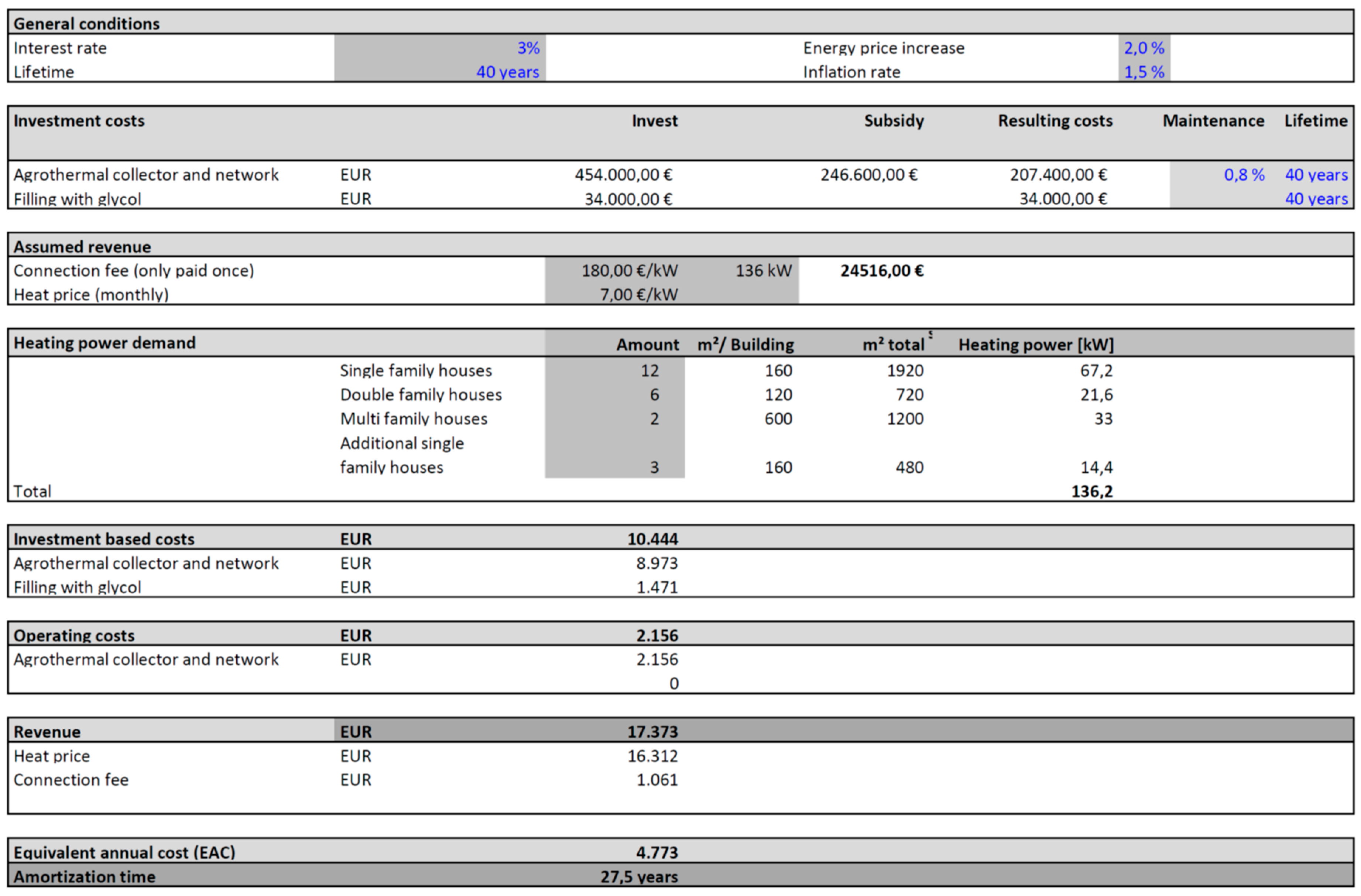
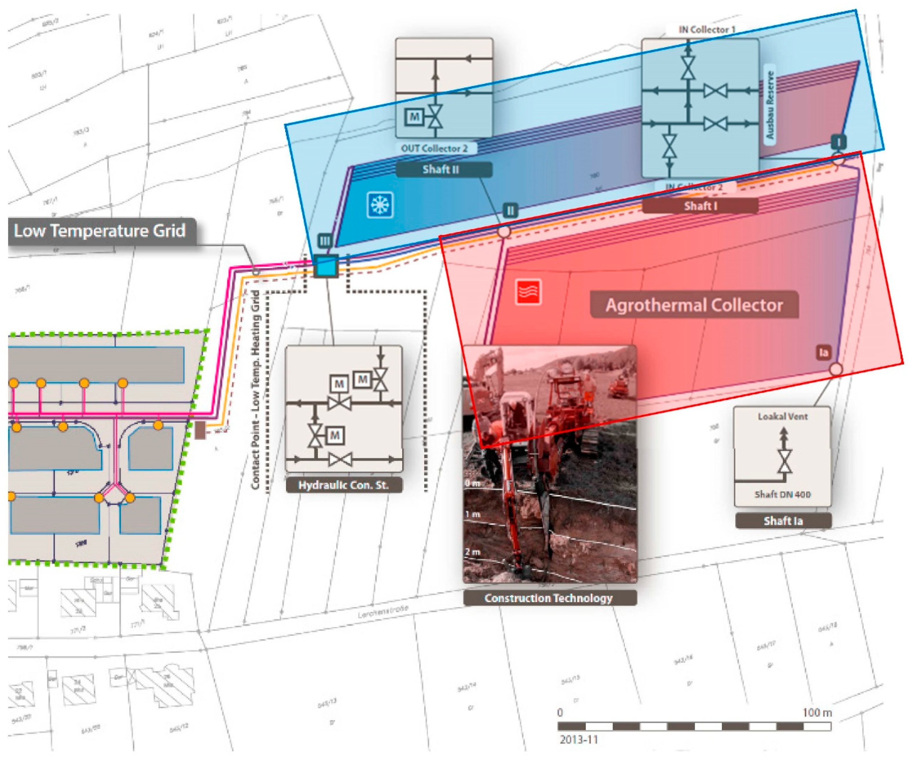
Initially, costs of 240,000 € were calculated for the construction of a 15,000 m² collector field. A supplementary 34,000 € would have been necessary to fill the grid and the collector with monoethylene glycol. For the construction of the DHC network, common costs of 350 €/m were assumed. To boost this novel technology, a subsidy of 246,000 € was granted within the federal German research project EnVisaGe. The collector field was planned in two construction phases to handle the growth of the Plus-Energy settlement (see Figure 2).

Unfortunately, the collector system was in a prototype state, which increased project costs consequently. Higher costs for transport of machinery and monitoring equipment installation also contributed to this issue. In total, the final costs of the first collector construction phase (Figure 2, blue collector) and its implementation were as high as originally planned for both construction phases at around 240,000 €, which resulted in specific costs of 54.5 €/m². Fortunately, trial operation of the low temperature DHC network showed that the ground’s actual heat transfer rate was higher than estimated in the planning phase. Thus, the first installed collector field of 4400 m² proved to be sufficient to support the first planning phase of 23 buildings. It is estimated that the construction costs could be reduced by 50% to 70% for further systems of the same type [22].

2.2. Settlement Heat Demand

The Plus-Energy settlement “Vordere Viehweide” spreads over 25,000 m² of land area, without the agrothermal collector field. Twenty-three buildings complying with the German KfW-55 standard are connected to the low-temperature DHC network. KfW-55 requires each building’s annual demand of primary energy to be equal or less than 55% of the demand of a new building with the same geometry, according to German energy-saving regulations. In addition, stricter regulations are put directly on the properties of the building’s thermal envelope. This results in a building-specific energy demand of 55 kWh/m². The settlement’s estimated annual heat demand for space heating and DHW (domestic hot water) is 340 MWh, resulting in 255 MWh of heat demand on the network side when assuming an average heat pump COP (coefficient of performance) of 4. Approximately 60% of provided energy is used for space heating, and the remaining 40% is used for DHW heating. The houses are equipped with underfloor heating systems, resulting in low supply temperatures. The decentralized heat pumps increase the low-temperature DHC network’s temperature to temperatures between 30 and 40 °C for space heating, with an estimated return temperature from the underfloor heating system of 6 K to 10 K lower than the supply temperature. The prepared DHW temperature is aimed to be around 50–55 °C [22].

2.3. Heat Supply by a Novel Agrothermal Collector Field with Low-Temperature DHC Network

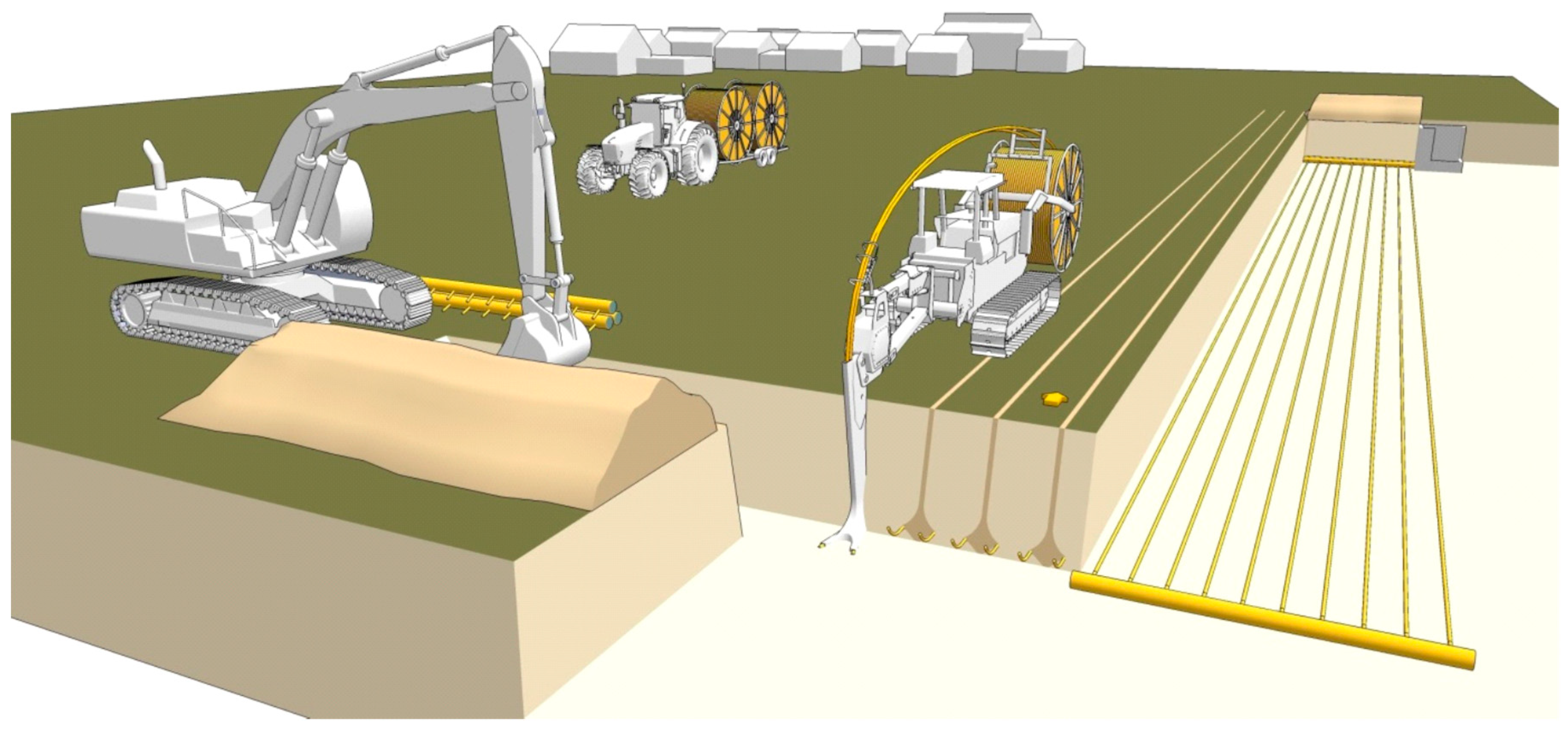
Despite the plan to include waste heat from chillers, at present the heat supply of the low-temperature DHC network comes solely from the very shallow agrothermal collector field with a size of 4400 m². The agrothermal collector field consists of pipes that lie in parallel to each other at a distance of 0.5–1 m. They were laid into the ground at a depth of approximately 2 m with a special plough (see Figure 3). This allows a very fast and easy installation of the collector pipes with no need for extensive earthwork, and this maintains the soil stratification. The pipes are also located far below the plant roots, not affecting the agricultural yield due to lower soil temperatures [22].

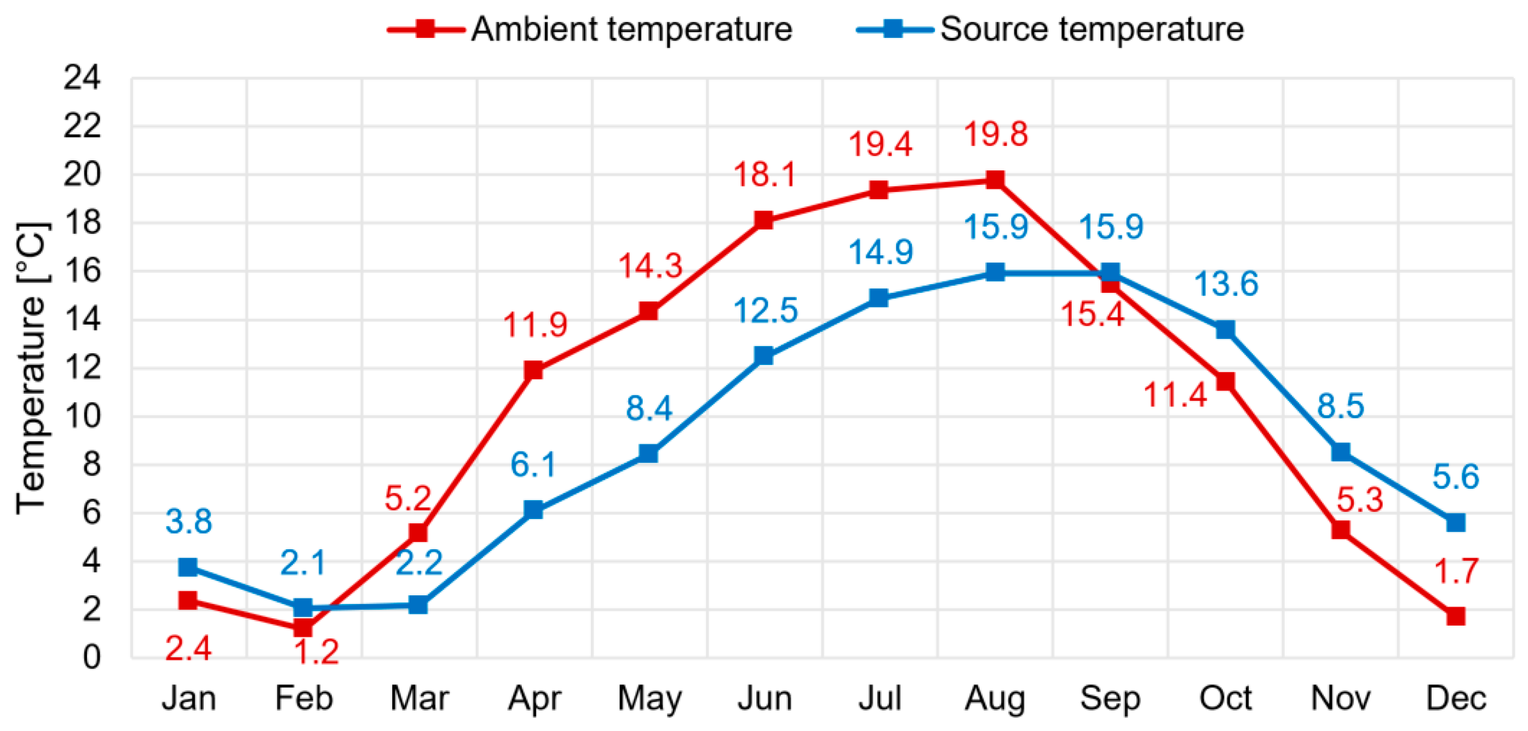
As it can be seen in Figure 4, the supply temperature of the low-temperature DHC network changes over the year, following a seasonal profile with a lag of approximately 1–2 months. The reason for this is that the geothermal collector is laid just 2 m below the ground surface, which allows the seasonal conditions to have a direct influence on the ground and thus on the collector transfer fluid temperature.

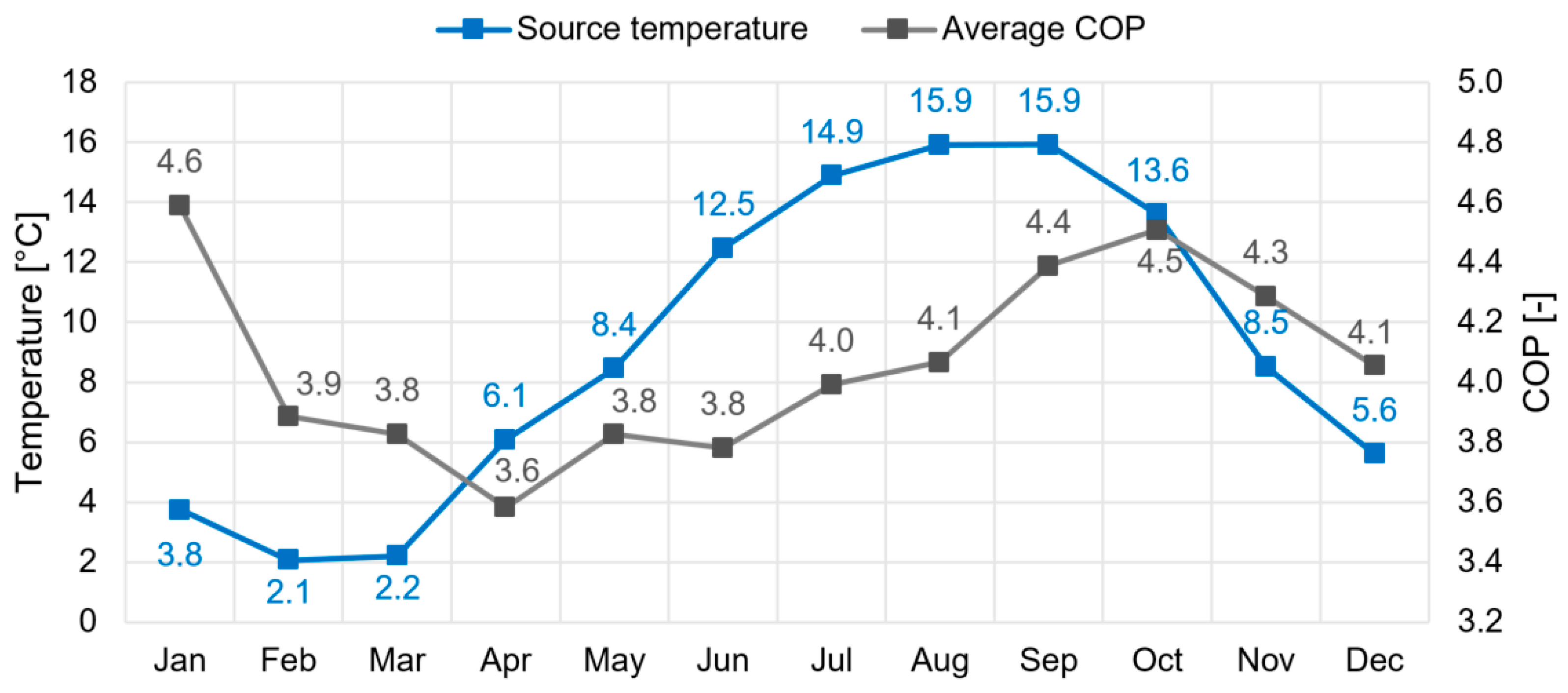
Figure 5 shows the monthly average COP value of six heat pumps for which detailed monitoring data on the electrical and thermal side (5 s measurement interval for the electrical side and 30 s for the thermal side) has been collected. It shows that the heat pumps’ COP depends on the low-temperature DHC network supply temperature. Even during summer when the COP should be lowered since only DHW is prepared at a higher less efficient temperature level, the effect of the supply temperature is stronger. The best COP values are generated in October when the supply temperature of the DHC network is “high” and at the same time the space heating demand increases. This leads to high COPs. In January, the supply temperature is yet high enough and the space heating demand exceeds the DHW by 90%, which also leads to high efficiencies. In May and June, when the space heating demand is very low and the supply temperature is not that high, lower COP values are generated. The lowest efficiency results by the end of the heating season in Germany in March/April. Then, the supply temperature is very low, and the heating demand is still very high.

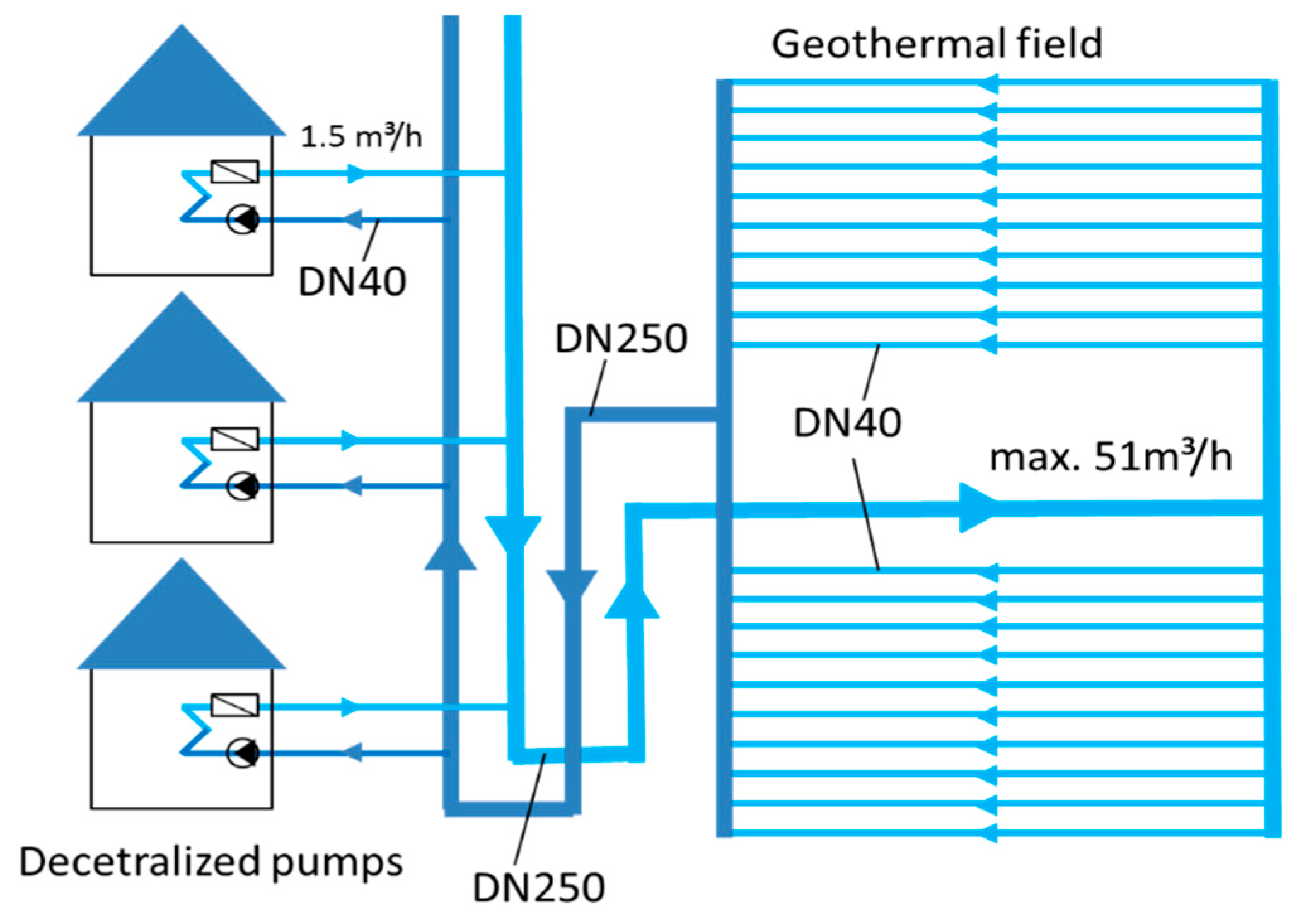
The entire low DHC network consists of a two-pipe system with a large diameter of DN250 (see Figure 6). The total network length is about 500 m. There are several reasons why the pipes are oversized. One is that the network was planned with a future extension in mind. In addition, the piping of the network works as a thermal buffer, no central circulation pump is utilized, and the pressure drop should be as low as possible. Since there are no thermal losses, no insulation is required, which is reducing the costs of oversized piping. At present, the buildings’ peak heat demand is at around 186 kW, resulting in a network-side peak heat demand of 140 kW (at a COP of 4) and a flow rate of about 32 m³/h [22].

Within the low-temperature DHC network, a 20% monoethylene glycol/water mixture is used (see

Table 2. Physical properties of the monoethylene glycol—water mixture circulating in the district heating (DH) loop in Wüstenrot [23].

Property	Value	Unit
Monoethylene glycol concentration	20	%
Freezing point	−8	°C
Reference temperature, Tref	10	°C
Density at Tref	1028	kg/m3
Specific heat at Tref	3.97	kJ/(kg K)
Dynamic viscosity at Tref	2	10−3 Pa s

). There is no need for a permanent circulation, because even when the circulation stops, the ground temperature remains available. Thus, the low-temperature DHC network’s circulation is turned on and off by the individual heat pumps. Every building is heated by decentralized heat pumps in combination with thermal buffer storages, of which some are controllable. The installed heat pumps have a thermal power output between 6 and 20 kW, depending on the building size. Each decreases the network fluid temperature between its inlet and its outlet by 4 K with an annual COP of around 3.8–4.6 [22].

Building owners were obligated to install heat pumps, PV systems, and thermal buffer storages, and to connect to the low-temperature DHC network, but they could choose the systems manufacturer and building services engineering planner by themselves. This resulted in a variety of different system combinations, resulting in more knowledge of the various combination’s behavior, but also in a higher construction workload and in higher costs, especially for the installment of the monitoring equipment.

2.4. Geothermal Monitoring

As mentioned above in Section 2.1, the existing agrothermal collector field excelled the assumed values for the heat supply of the DHC network. As a reminder, the primary specific heat capacity of the collector field was estimated at between 40 and 70 kWh/m² per year with the assumption that 40 kWh/m² per year could be extracted from the soil a total size of around 6500 m² would have been necessary to cover the low-temperature DHC network’s total heat demand of 255 MWh. Thus, that a size of only 4400 m² of collector area actually can serve the complete heat demand of the connected 23 consumers had to be investigated in detail.

To map the thermal behavior of the agrothermal collector field and the effects of the temperature and humidity conditions of the tethered soil was the one main objectives of the geothermal monitoring planned for Wüstenrot. To balance the needs of accuracy versus technical and financial aspects of the monitoring, only one collector tube was equipped with several thermal and humidity sensors, as shown in Figure 7.

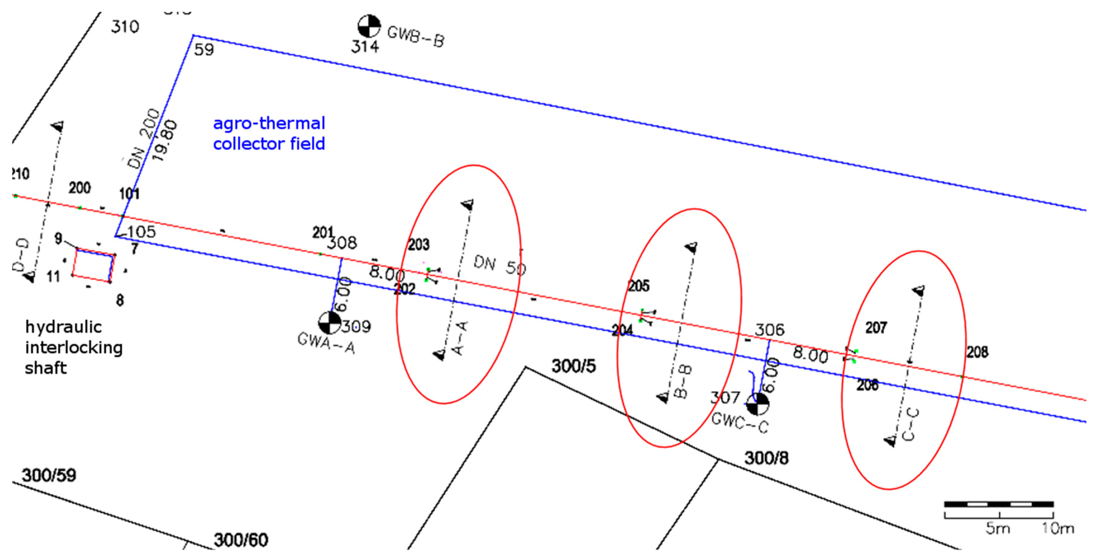
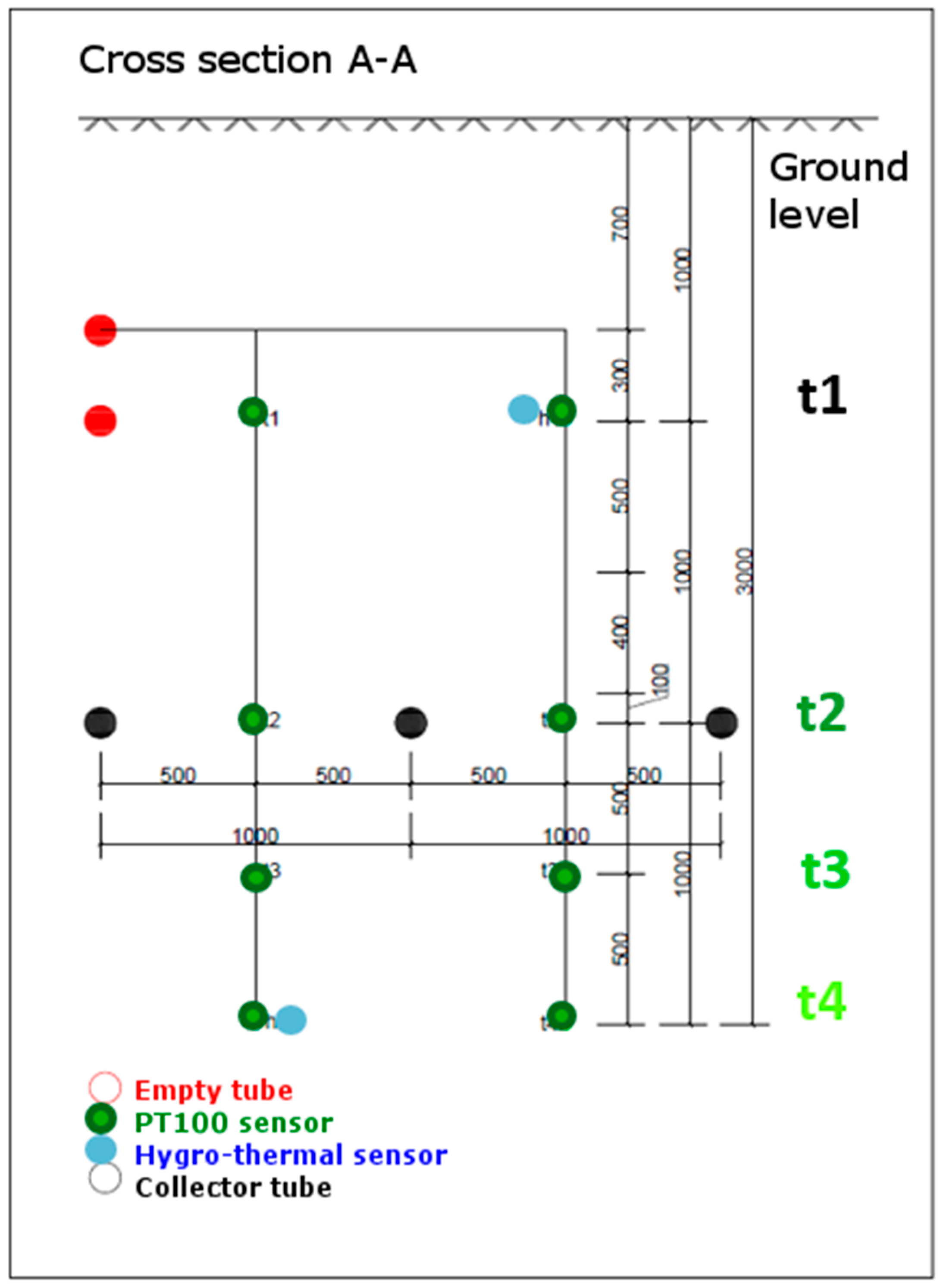
Three horizons (A-A, B-B, and C-C) of temperature and humidity measurements along one collector pipe (red line) were installed (Figure 7). The metering point horizon A-A is approximately 25 m far from the hydraulic interlocking shaft of the collector, displayed as a red rectangle in the lower left side of the scheme. The distance among the horizons A-A, B-B and B-B, C-C is equal: 20 m each. All sensors are connected to the data acquisition in the interlocking station by wires. For fast and easy installation of the measurement setup, all sensors were preinstalled on slotted filter pipes with a total length of 4 m each. One measurement horizon consists of two of these tubes buried vertical in the soil (top edge 0.5 m under ground level, see Figure 8).

The distance between the collector tube and its metering points is about 0.5 m on the left- and right-hand sides of the tube. For the mounting of the sensors, slotted filter pipes were chosen because of their hydraulic behavior. These tubes are hydraulically “transparent”, which means that there is almost no influence of the groundwater flow nearby the installation. The supposed groundwater flow through the collector field has been logged by the three metering points GWA-A, GWB-B, and GWC-C. At all three metering points, the level of groundwater can be measured down to a depth of 4 meters under ground level. All the metering points shown in Figure 7 were calibrated by GPS measurements and precise leveling of the geographical height.

With the three sensors GWA-A to GWC-C, the level of the groundwater can be measured within the collector field. With their exact height above sea level and the pressure differences caused by the varying water pillars over the sensors at the bottom of the installation, the gradient of the groundwater level can be calculated. Combined with the properties of the soil, the velocity and the direction of the groundwater can be derived.

In a first try to explain the significant increase of the thermal capacity compared to the design assumptions of the collector field, a simplified investigation was done.

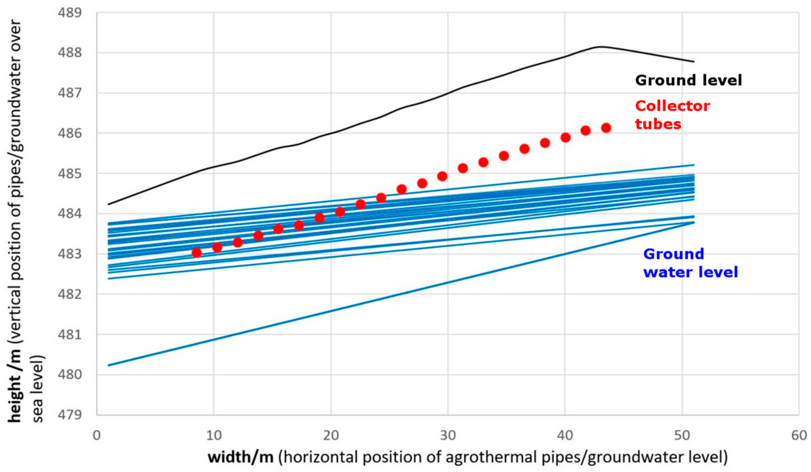
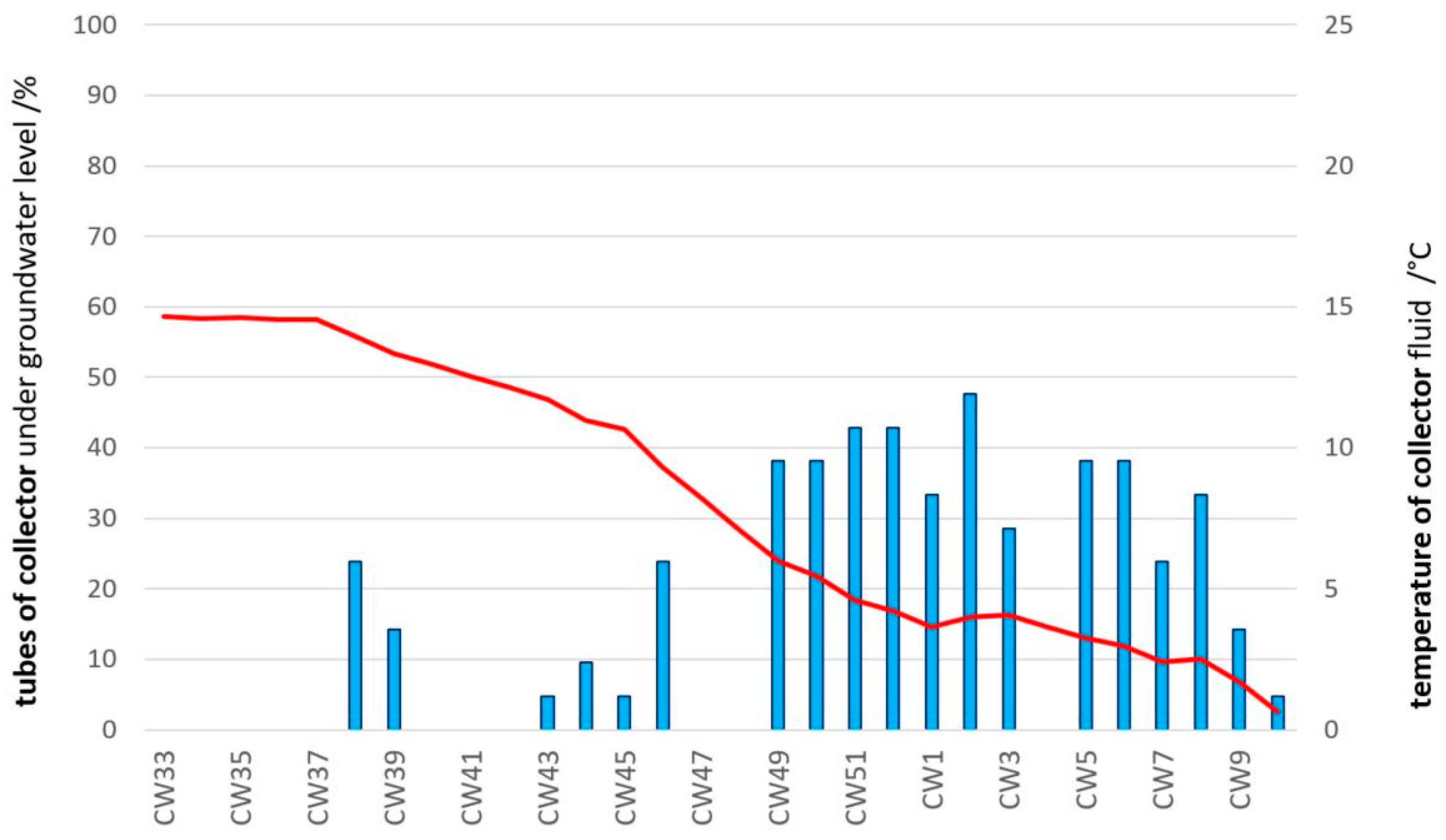
A one-dimensional groundwater gradient between metering point GWB-B and GWC-C was calculated for each week in the 2017–2018 heating season. In Figure 9, these gradients are shown as blue lines. The red dots in the scheme represent the height of the 21 collector tubes in the cross-section GWB-B/GWC-C. The red dots that are below the blue line are under the groundwater level, while the others are above (the black line on top of the red dots is the vertical position of the ground level). Each blue line represents the groundwater level for a duration of one week. In Figure 10, the cover percentage of the collector field by groundwater level (blue bars) is plotted against the time by adding the supply line temperature of the DHC network as red line. This graph shows that during the 2017–2018 heating season, a significant amount of the collector field is below the groundwater level. This results in a higher heat capacity [24] and heat conductivity [25] of the tethered soil, while in the summer season the dry soil has higher temperatures, which could be read from the corresponding supply line temperature of the DHC network (red line). The constant high COPs of the connected heat pumps shown in Figure 5 and the high thermal performance of the agrothermal collector can be explained as a consequence of either the high temperatures of the heat source (soil) during the summer season or the high heat capacity and conductivity of the soil during the heating season.

2.5. PV System

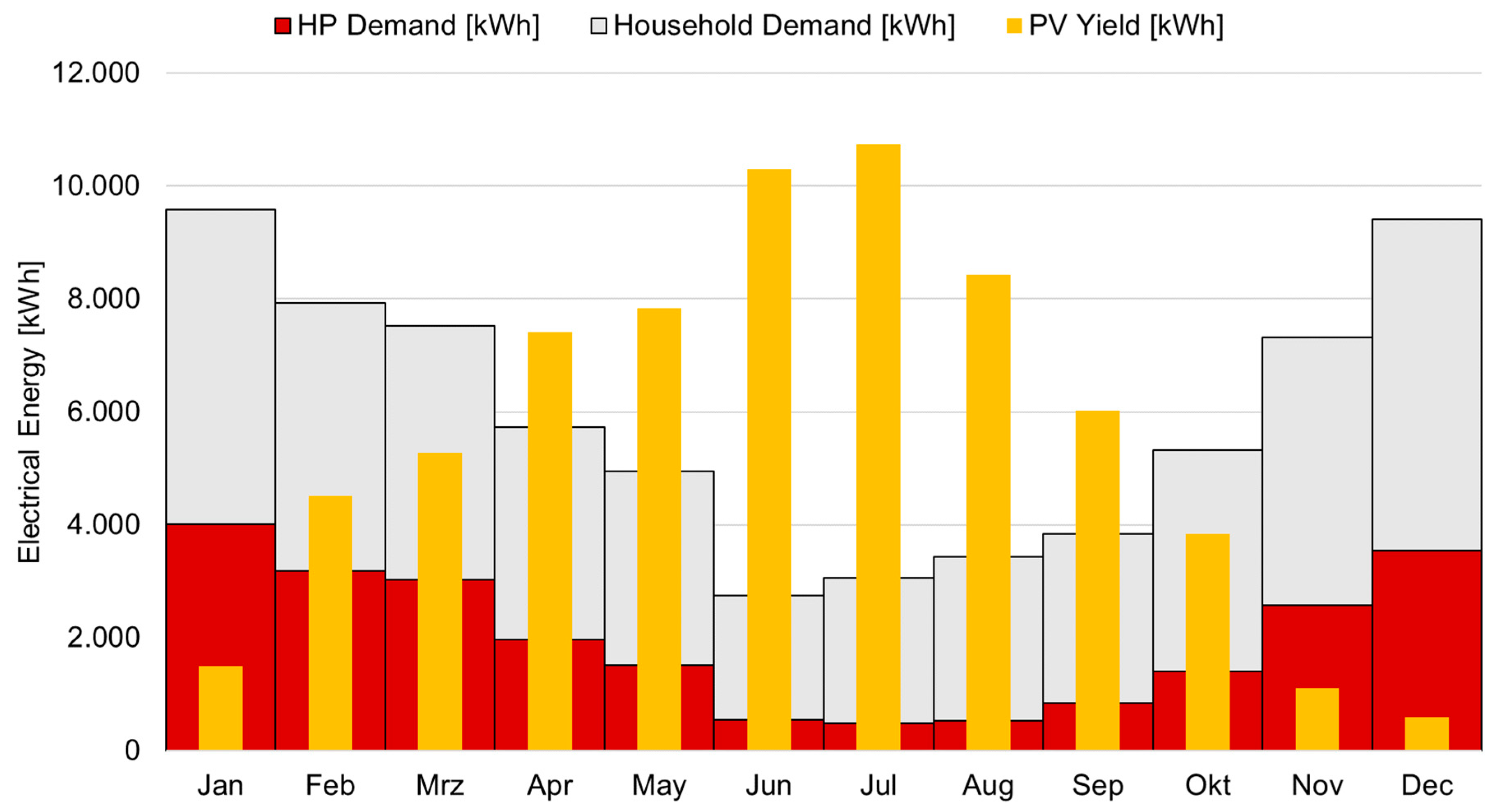
All buildings are equipped with PV systems with a peak power output in between 5 and 28 kW_p. In total, approximately 230 kW_p are installed, leading to an annual PV electricity production of approximately 210 MWh. The data available and simulations suggested that the PV electricity production contributes to about 30% of the buildings electricity consumption including heat pump and household demand (see also Figure 11). On the balance sheet, it can be seen that the PV production of November, December, and January is not high enough to fit to the heat pump. To solve this problem, a seasonal electrical storage system as described for the case of Wüstenrot in [26] or bigger PV systems is needed. Half of the year, the whole household’s electricity demand can be capped with PV on the balance sheet.

Six of the buildings are equipped with battery storages of 5 kWh capacity, increasing self-consumption by about 20% [26,27]. Regarding the fact that the electricity price for residential users in Germany is around 0.29 € and the feed in tariff is approximately 0.11 €, this becomes increasingly important.

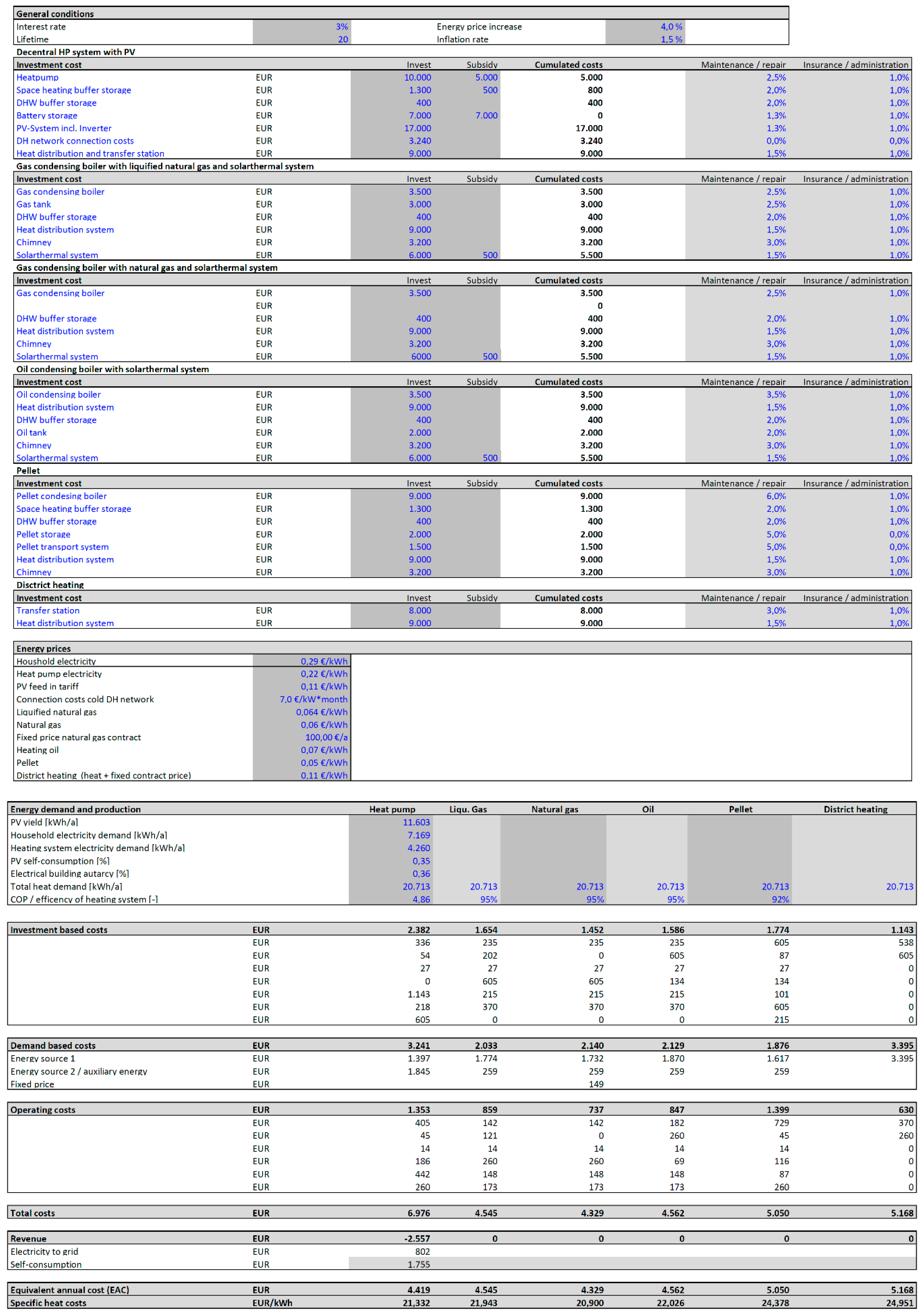
2.6. Economical Assessment

The dynamic profitability calculation was carried out based on the annuity method according to the guildeline VDI 2067 “Economic efficiency of building services systems” [28]. Furthermore, to take into account energy price increases and inflation, the procedure according to [29] was used.

The economic feasibility is calculated in terms of EAC (equivalent annual cost), which represents the annual cost of owning, operating, and maintaining the different system components. The EAC are calculated by Equation (1):

$$EAC={{\displaystyle \sum }}_i{P}_i+m_{om}*{{\displaystyle \sum }}_{i}O{M}_i+m_f*{{\displaystyle \sum }}_i\left(c_{f,i}*Q_{f,i}\right)+{{\displaystyle \sum }}_i{P}_i-{{\displaystyle \sum }}_i(R_i*m_{f,i})$$

(1)

with $O{M}_i$ [€] as the sum of the yearly fixed and variable operation and maintenance costs of the component $i$, $Q_{f,i}$ [MWh] as the amount of energy used by the component $i$, $c_{f,i}$ [€/MWh] as the price of the energy source/carrier used by the component $i$, and $R_i$ [€] as annual revenues such as the PV electricity fed into the grid, money saved through self-consumption or low-temperature DHC network connection fees.

Thereby, $P_i$ [€] (annualized capital cost of investment of the specific system component ($i$) is calculated by the following Equation (2):

$$P=PV*\frac{r_i}{1-{\left(1+r_i\right)}^{-n}}$$

(2)

where $PV$ [€] is the present value of the total investment, also including present revenues such as fixed priced connection fees, $r_i$ [%] is the yearly interest rate, and $n$ [year] is the investment lifespan.

The increase in operation and maintenance costs is taken into account via the factor $m_{om}$ [-], which is calculated by the following Equation (3):

$$m_{om}=\frac{1+r_{om}}{r_i-r_{om}}*r_i*\frac{{\left(1+r_i\right)}^n-{(1+r_{om})}^n}{{\left(1+r_i\right)}^n-1}$$

(3)

where $r_{om}$ [%] is the annual increase in operation and maintenance costs. The increase in energy prices costs is taken into account via the factor $m_f$ [-] that is calculated by the following Equation (4):

$$m_f=\frac{1+r_f}{r_i-r_f}*r_i*\frac{{\left(1+r_i\right)}^n-{(1+r_f)}^n}{{\left(1+r_i\right)}^n-1}$$

(4)

where $r_f$ [%] is the annual increase in energy prices. This factor is also partly credited to the annual revenues for the reduction of grid electricity purchase due to self-consumption. The grid feed in tariff for PV electricity is assumed to be fixed over the considered time period of 20 years.

3. Monitoring System and Optimized Building Operation

Within the Plus-Energy settlement “Vordere Viehweide”, the building owners had clearly defined targets regarding building efficiency, heating systems, and PV systems (every owner had to install a PV system of sufficient size in order to reach the Plus-Energy status on a yearly balance). Despite this, the individual system components and layouts could be freely chosen, leading to a variety of hydraulic layouts and different types of manufacturers. This made the installation of monitoring equipment quite difficult, as each building system is different. Conversely, it also offers the opportunity to obtain the data of and experience various system combinations. Within six buildings, all the thermal and electrical energy flows and temperatures are monitored in high resolution (5 s electrical, 30 s thermal) and their energy systems, especially their heat pumps, are controllable by a local energy management system. For those six buildings, an implementation of DR and DSM measures is carried out with various goals:

• Optimization of self-consumption
• Application of flexible electricity tariffs
• Aggregated power market participation

Thereby, flexibility is provided by overloading the thermal storages and buildings. This requires simulation-based prediction and optimization. In the literature, for prediction and optimization purposes, various approaches exist, ranging from black box self-learning algorithms over gray box RC models to dynamic white box building models, providing different advantages and disadvantages regarding computational time, prediction accuracy, and adaptability [30]. In the field of energy engineering and science, three different optimization approaches are widely in use: mixed-integer linear programming (MILP), dynamic programming (DP), and metaheuristic algorithms such as genetic algorithms (GA) [31]. One approach is to use dynamic building models such as EnergyPlus to create optimized set point schedules for the following day, allowing significant electricity cost savings [32,33]. In the case of the Plus-Energy settlements’ individual buildings, a hybrid approach is implemented. Thereby, a local energy management system together with a cloud-based simulation and prediction software prototype is used to enable DR and DSM measures. Within that, the heat pump operation is optimized and scheduled according to the predicted PV yield, heating, and electrical household demand and partly by external activation or pricing signals.

For monitoring and control purposes, the communication protocols at the level of the devices are the following:

• For the heat pumps, either the potential-free contact to switch them on or off (historically used by grid operators to switch off the heat pump for a certain time period per day) or ModBus TCP being the most advanced external control interface;
• For the battery charge control, a ModBus TCP protocol is used for the communication with battery inverter and to gain the charging level of the battery;
• For the PV Systems, ModBus TCP is also used.

To collect the data from the various installed monitoring devices, different interfaces from simple thermocouples that are connected to the I/o-modules over analogue interfaces up to different bus protocols such as ModBus TCP and ModBus RTU as well as proprietary bus protocols are used.

All monitoring data is stored in a cloud-based MySQL database with dedicated structure to be accessed via the monitoring software MoniSoft [34].

3.1. Prediction Approach

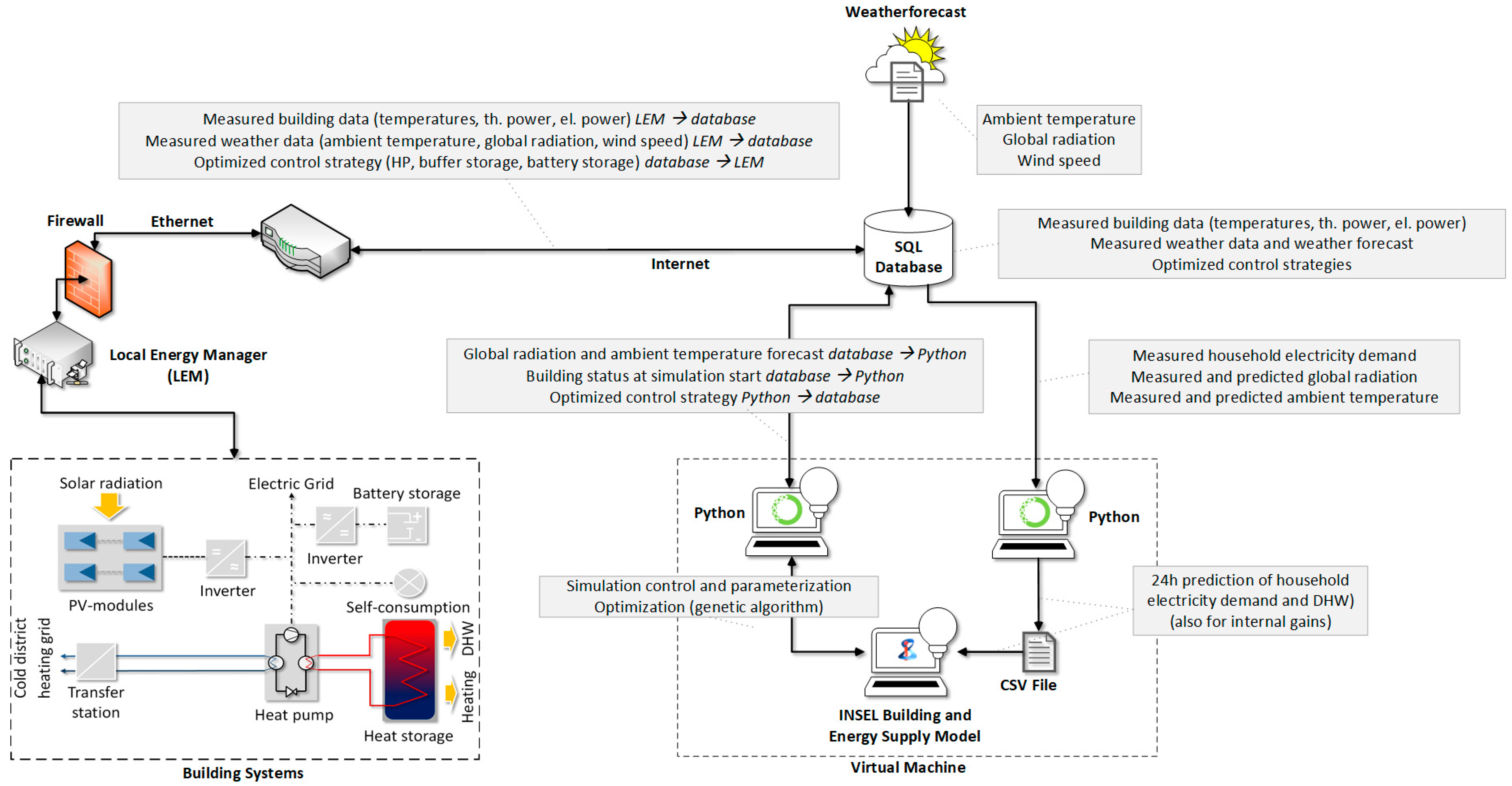
For the load forecast and generation of optimized daily heat pump operation schedules, the simulation environment INSEL (Integrated Simulation Environment Language), the user-driven demand prediction algorithms and the optimization (both realized in Python) run in a cloud-based virtual machine. The communication between the simulation environment and the database is carried out by a Python script. This approach is also shown in Appendix A (Figure A1).

For the initialization of the simulation and optimization process, all relevant data (ambient, indoor, and buffer storage temperature, charging status of battery storage) are used as the simulation models starting parameters. For the predictive simulation, a 24 h forecast for ambient temperature and global radiation from a metrological data provider is used. The household electricity and DHW demand are predicted by an algorithm based on DTR (decision tree Regression), kNN (k-nearest neighbors), and k-means clustering, constantly trained by previous measured data. This approach is further described in Section 3.1.2.

3.1.1. Building Demand and Production

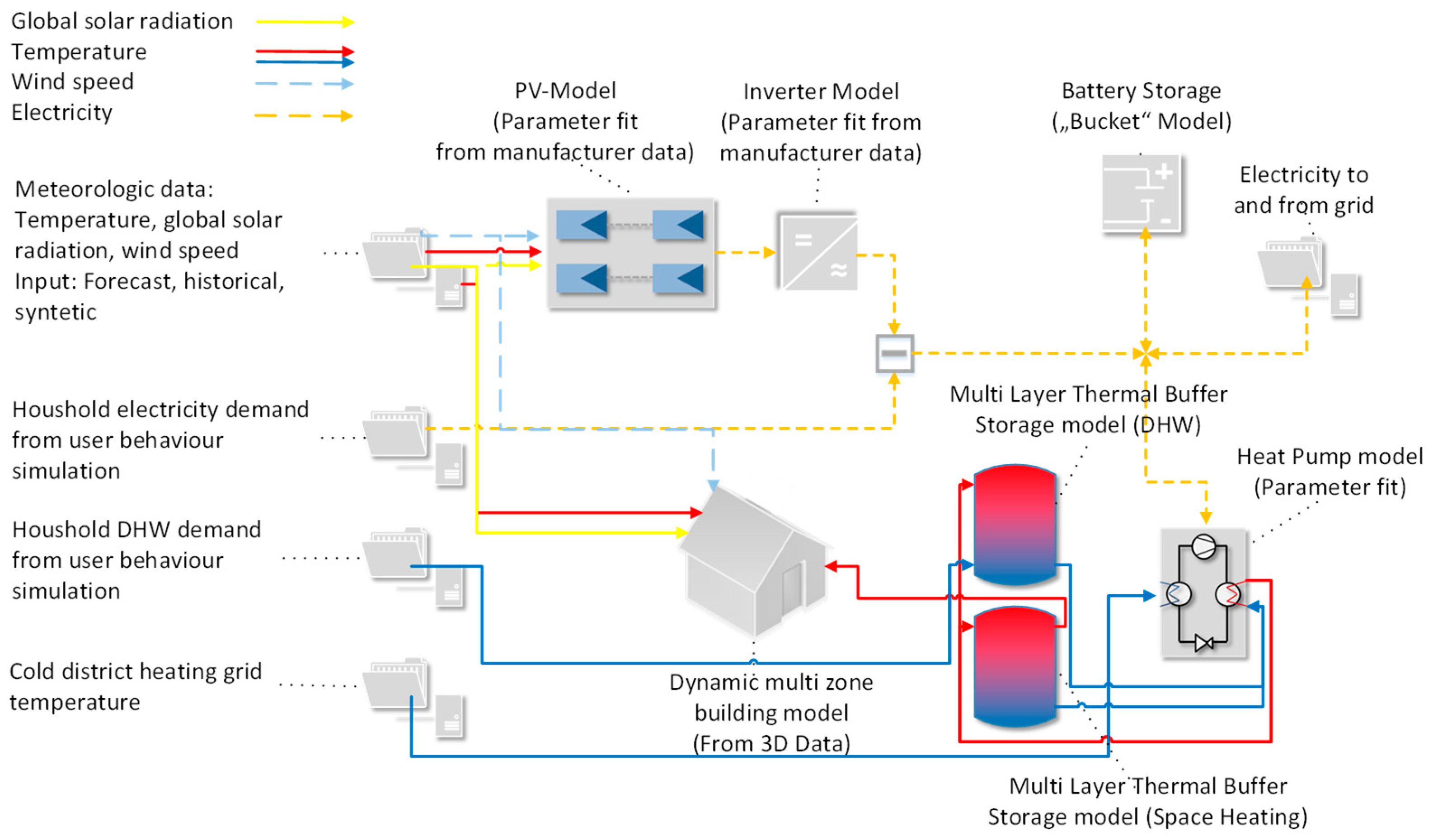
All systems and the thermal behavior of the building are dynamically modeled in the simulation environment INSEL [35]. The following Figure 12 gives an overview over all the components, their interaction, and the data flow. All the individual parts are described further below. A more detailed description and assessment of the model is also given in [36].

Dynamic Building Model

The utilized model provides a high level of detail while allowing for simplification at the data model level. It is based on the nodal method. This method is common for building simulations, especially when simulating multiple zone buildings. This approach also enables a good balance between the level of detail in the results and in the calculation time. The model contains a one-dimensional numerical solution of the heat conduction equation for each wall. Additional nodes contain room air and windows. Long-wave radiative exchange between the room surfaces is also considered.

Heat Pump

The applied model simulates the compressor’s behavior based on a polynomial function (according to norm DIN EN 12900). The heat exchangers on the evaporator and condenser side are resembled with the NTU method (number of transferred units). This simplifies the calculation process, because no complex calculations due to complicated streamlined shapes have to be carried out.

Thermal Buffer Storages

Within the thermal buffer storage model, each layer is modeled physically. Heat conductivity between the layers is calculated. Thermal losses are added to the suitable building zone.

PV Modules and Inverter

The modules are represented by a two-diode model that is suitable for mono- and polycrystalline Si (silicon) as well as for CIS (copper indium gallium selenide) modules. The parameters are created via a parameter fit according to module characteristic curves. The inverter is also represented through parameter fit by characteristic curves provided by the manufacturer. The PV modules are linked to a MPP (Maximum Power Point Tracking) loop.

Battery Storage

The battery storage model is kept simple. It does not simulate the electrochemical process of the battery. The charging and discharging efficiency, power, inverter efficiency, and self-discharge are considered. The aging effect is considered dependent on number of cycles (linear aging coefficient).

3.1.2. User-Driven Demand

The prediction of the household electricity demand can contribute to an increase in the efficiency and as well to an optimized operational sequence of the buildings’ systems [37,38]. In this context, the extent to which the use of machine learning approaches can contribute to the prediction of household electrical power demand is investigated. The methods used are kNN and DTR.

kNN Regression

Regression using the kNN method is one of the fastest and easiest tools for machine learning. One reason for this is the low complexity of the model. While many other methods of machine learning train a function, the kNN regression stores the individual data points of a selected training data set. In a query, the input data is compared with the training data, and a point that comes as close as possible to the input is delivered as output. This point represents the nearest neighbor. It is possible to select several neighbors, whereby in a very simple model, the mean value of the Euclidean distance is delivered as the output point. However, it is also possible to use other parameters that allow certain data points to have a greater influence on the result than others.

For the parameterization of the method, the number of neighbors, the weighting of the data points, and the algorithm to detect the nearest neighbors, as well as the regularization can be used [30,39,40].

As already mentioned above, the model is a very simple one, which can produce relatively good predictions with a small number of characteristics (input data such as temperature, pressure, and irradiation). Furthermore, trends can often already be identified with this method, which is why this algorithm can be a suitable tool for generating initial results due to its fast programming [41].

k-Means Clustering

The method k-means represents a cluster analysis and is assigned to the spectrum of unsupervised learning in the field of machine learning. The method is unsupervised, since the algorithm does not receive test data for its categorization, which would allow it to validate itself. Thus, clustering assigns similar data points to a category chosen by the algorithm itself.

The algorithm first determines a relative random center of one or more clusters. Then, it follows the allocation of the next data points to the centers of the respective clusters. The allocation of the data points affects the position of the mean value. These two steps are performed alternately until all data points have been assigned to the cluster centers. Ideally, the cluster center is located in the center of a data point cloud at the end. The disadvantage of using the k-means method is that the cluster size of the different groups is assumed to be the same. This assumption is also used to determine the boundary of the cluster, which separates the two groups exactly in the middle between the centers of the clusters. However, here, neither the density nor the shape is taken into account. If the data cloud is a longish distributed point, the center and the boundary are wrongly defined. Here, other clustering methods are better suited [30,40].

The method can be adapted to the data by different parameters. The clusters to be formed can also be predefined [39,41].

DTR

Decision trees represent binary decision structures that can theoretically be run infinitely in order to carry out classifications. However, there are also methods in which several decision trees can be used for regressions. If you now imagine a tree, the basic data is the trunk from which the branches and leaves branch off. At the forked branches, the data is sorted by a yes/no questioning. Then, the data is further sorted out according to a sieve principle until the target classification has been reached. In this way, very complex models can be generated. High model complexity also leads to overfitting. The decision trees have to be cut for a certain elasticity of the prediction [39,40].

Data Preprocessing and Analysis

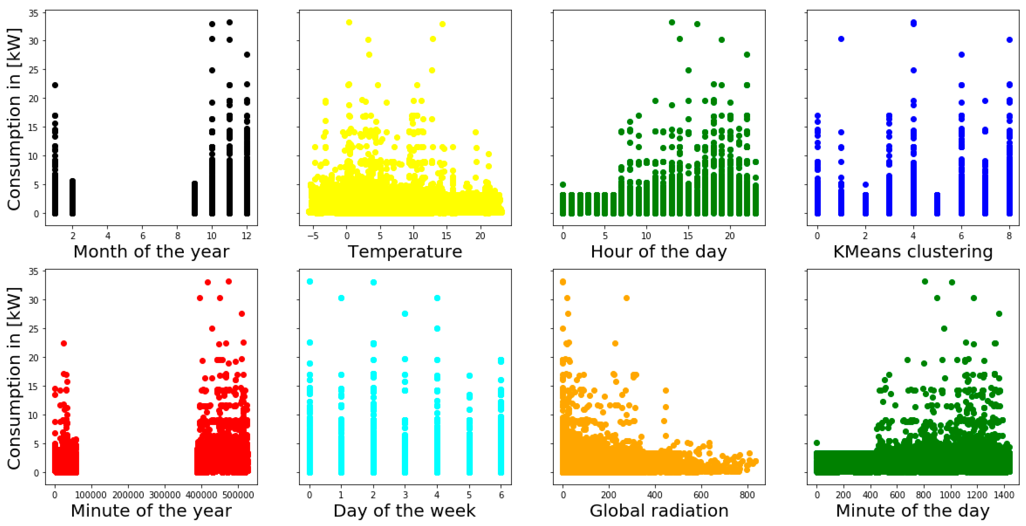
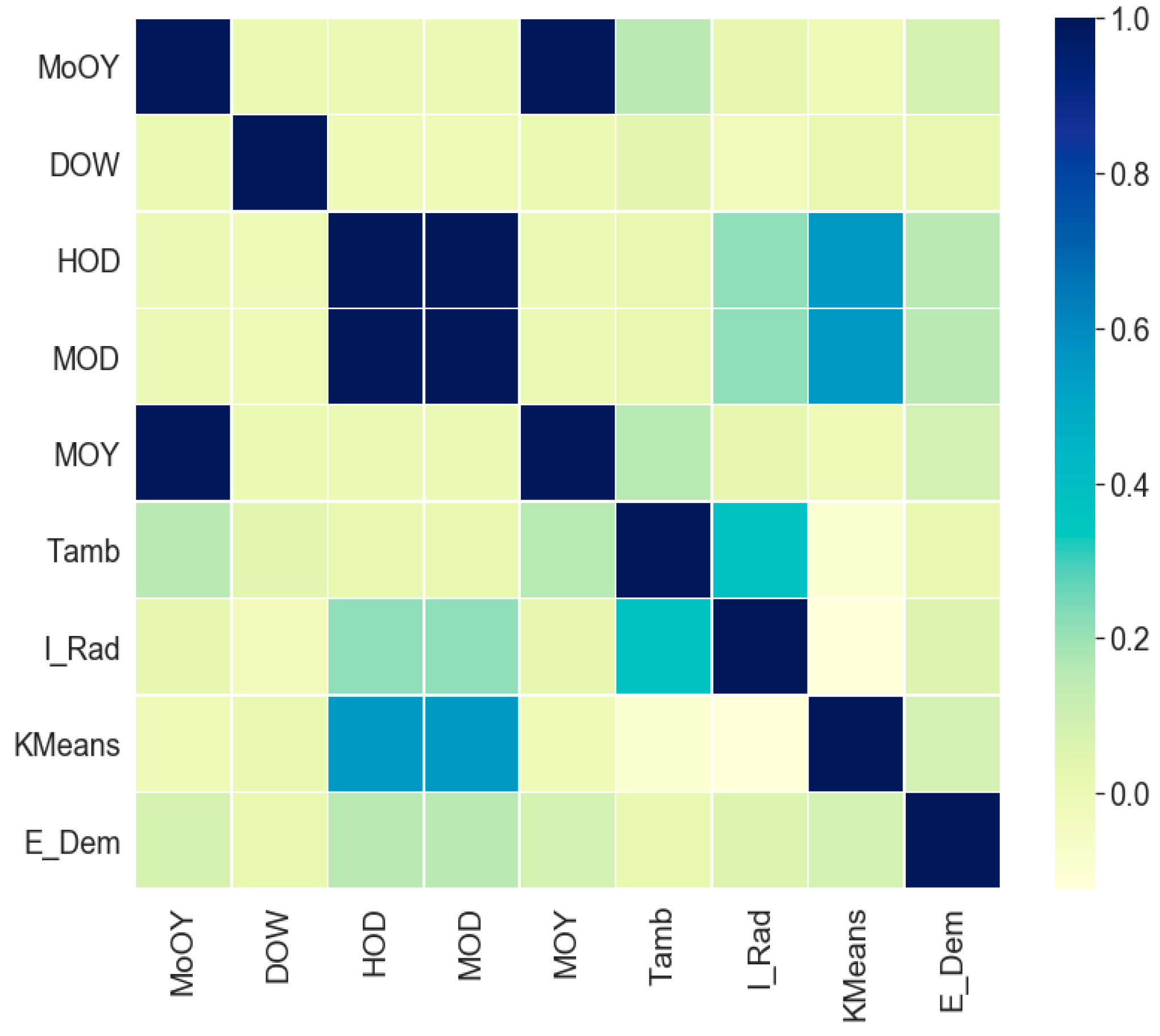
The data from project “Vordere Viehweide” is loaded as a CSV file into the program structure. This is a data preprocessing program. The time imported as UNIX time is used to generate characteristics such as month of the year (MoOY), day of the week (DOW), hour of the day (HOD), minute of the hour (MOH), and minute of the year (MOY). The other data that serve as characteristics are the ambient temperature (Tamb) and the global radiation (I_Rad) as well as the demand for the household electricity (E_dem) that serves as the target value. In addition, the data (without E_dem) is analyzed by a clustering method (KMeans) to classify the data. The dataset consists of data every minute for three quarters of a year. The ideal number of nine clusters was determined using a grid search. In a scatterplot (see Figure 13 and Figure 14), the training dataset (85% of the total dataset) of the respective characteristics (x-axis) is plotted with the target value (y-axis). This shows that the power requirement varies between the months and days of the week. In addition, the power requirement always increases only in the evening of the day. The temperature shows that a higher power requirement tends to be the case on colder days.

The clusters of the k-means will represent a classification of different commonalities that have the remaining characteristics. The clusters in which the power consumption is low and the clusters in which the power demand is high can be identified. Figure 14 shows as a heatmap the correlations (Pearson) between the characteristics. It can be seen that HOD and MOD have the highest Pearson correlation with 0.165. Then, we follow MoOY and MOD with 0.10–0.11. In addition, the clustering priority can be read from the representation, namely that it is strongly oriented to the hour of the day (HOD) and the minute of the day (MOD). The application is applied in Python and the scikit-learn library [41].

3.1.3. Experimental Validation and Prediction Inaccuracy

Evaluation

The predictive performance of the methods determined in this paper is evaluated with the statistical error interpretations the mean absolute percentage error (MAPE) and percentage mean deviation (MAE).

The mean absolute percentage error or MAPE represents the absolute percentage deviation of the values. Therefore, a particularly low value means a good reproduction of the regression model.

$$MAPE(\%)=\frac{100\%}{n}{{\displaystyle \sum }}_{i=1}^n\left|\frac{y_i-{\widehat{y}}_i}{y_i}\right|$$

(5)

The real value is subtracted from the forecast and divided by the real value. Thus, the sum of the individual deviations multiplied by 100% and divided by the number forms the percentage mean deviation (MAE).

$$MAE=\frac{{{\displaystyle \sum }}_{i=1}^n\left|\widehat{y_i}-y_i\right|}{n}$$

(6)

In many studies, MAPE is a popular way of evaluating forecasting methods for household electricity demand [37,42].

Eletrical Heat Pump Demand

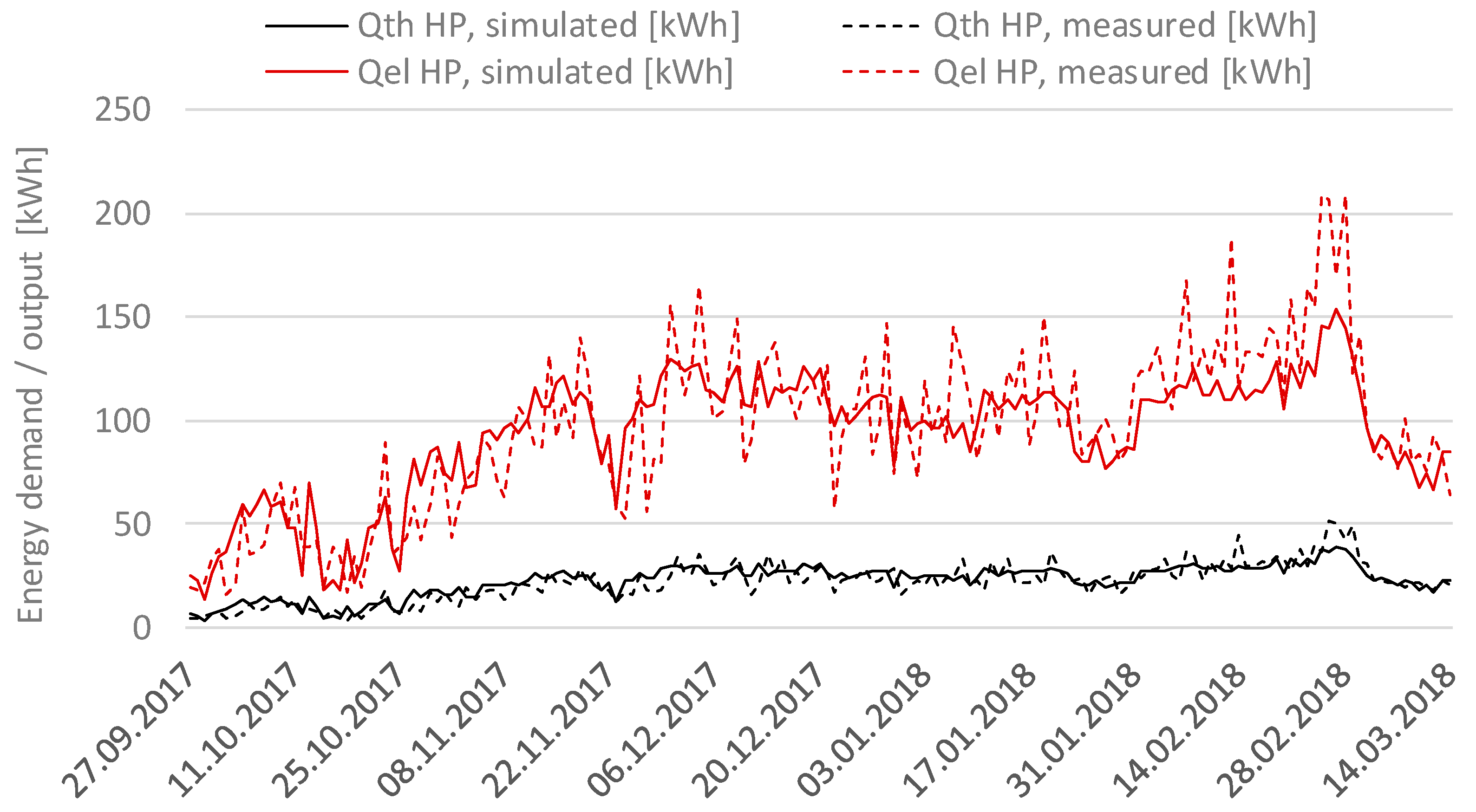
For validation purposes, simulations were carried out with metrological data (ambient temperature, global radiation) during the heating period of 2017/2018, including autumn, winter, and spring. During that period, the thermal heat pump energy output was 15,744 kWh (simulated) and 16,182 kWh (measured). Electrical heat pump energy demand was 3826 kWh (simulated) and 3691 kWh (measured). These results are also shown in Figure 15. 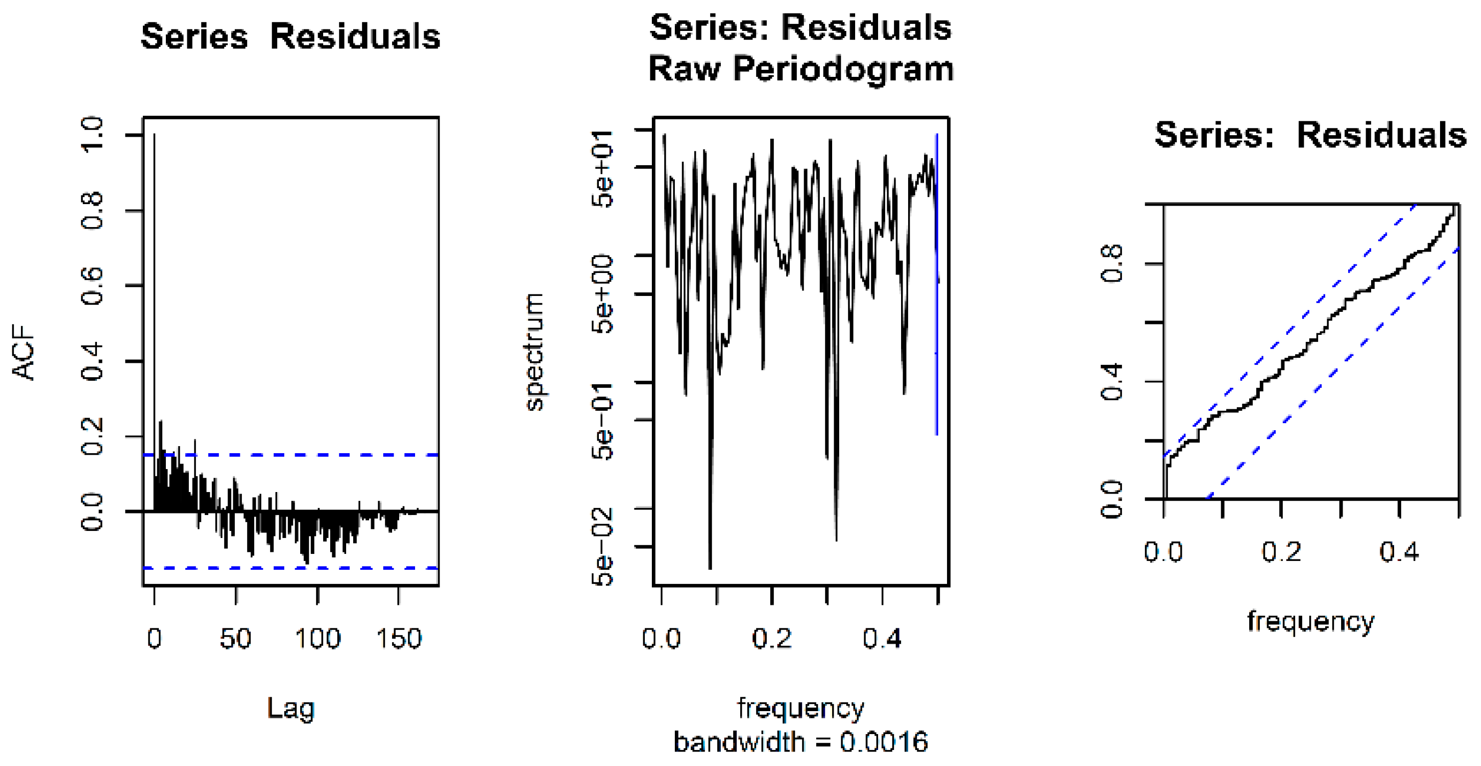Figure 16 shows the ACF (autocorrelation function) and the corresponding residuals plot. With a MAPE of 22.8%, the results show a good match on a daily basis as well as no periodic dependency regarding the ACF that would implement a systematic error.

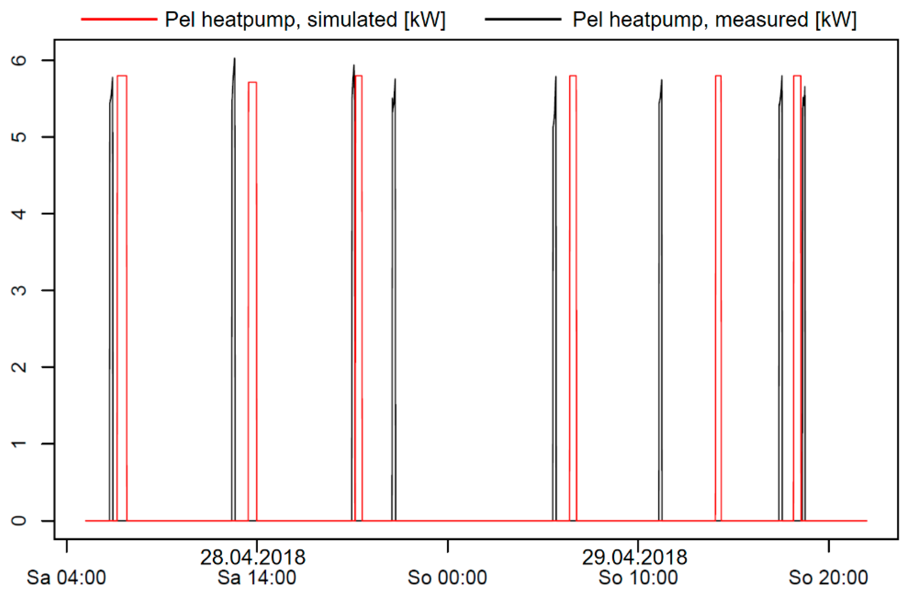
Figure 17 shows a comparison of the simulation results with the measured electrical power demand of the heat pump with a one-minute time resolution over the course of two days. The power peak and the durance of the heating process show a good match. Nevertheless, predicting the timing of the intervals is not always accurate, e.g., due to user behavior affecting the DHW demand and ventilation.

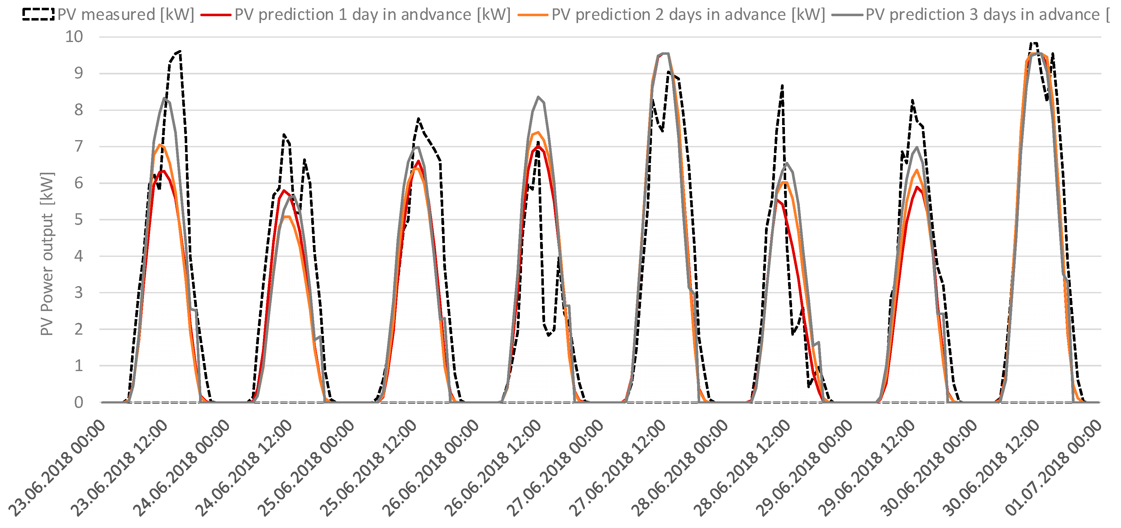
PV Electricity Production

For the predicted PV production baseline, the MAPE on an hourly basis between the PV power prediction and real measured data is 22.1% for a forecast one day in advance, 23.3% for a forecast two days in advance, and 27.5% for a forecast three days in advance (see Figure 18).

Household Electricity Demand

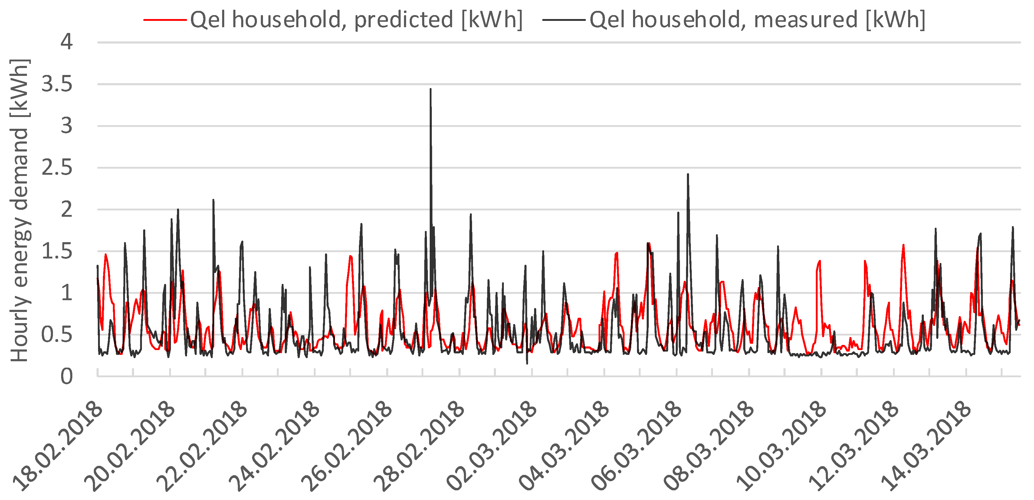
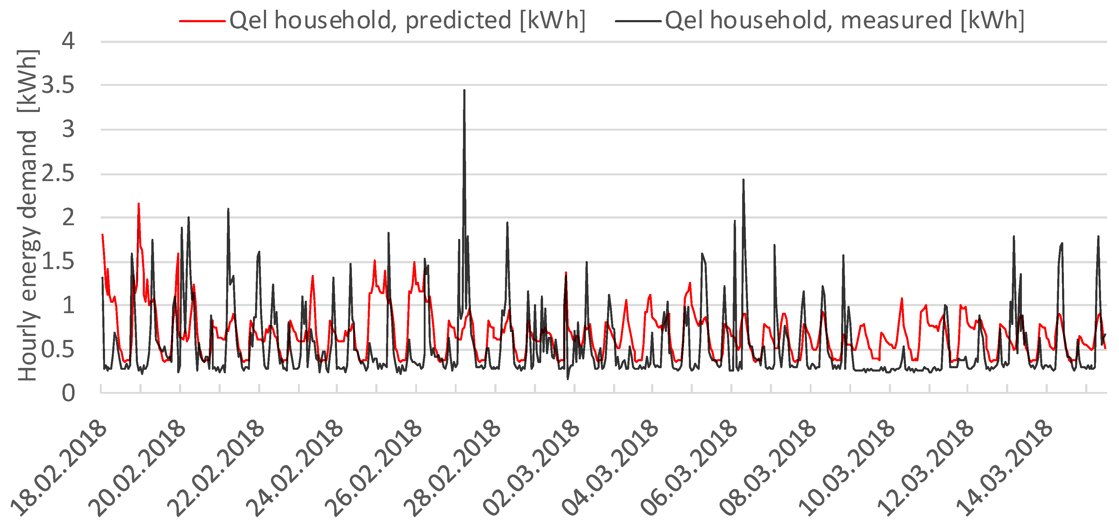
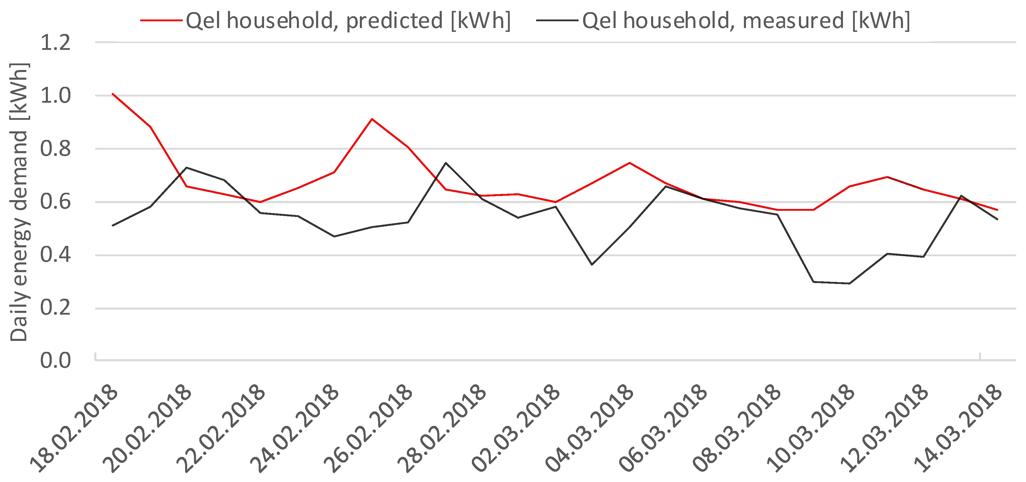
The models kNN and DTR are trained with 85% of the dataset and tested with the rest. The training of the models is optimized by a grid search. In Figure 19 the hourly kNN prognosis for the test data (612 h) is shown.

The frame of the prediction corresponds to about 25 days. The hourly course shows that the demand peaks of the prediction by the kNN method correspond to the actual ones but often show a shift on the x-axis. In addition, the load peaks are often over dimensioned.

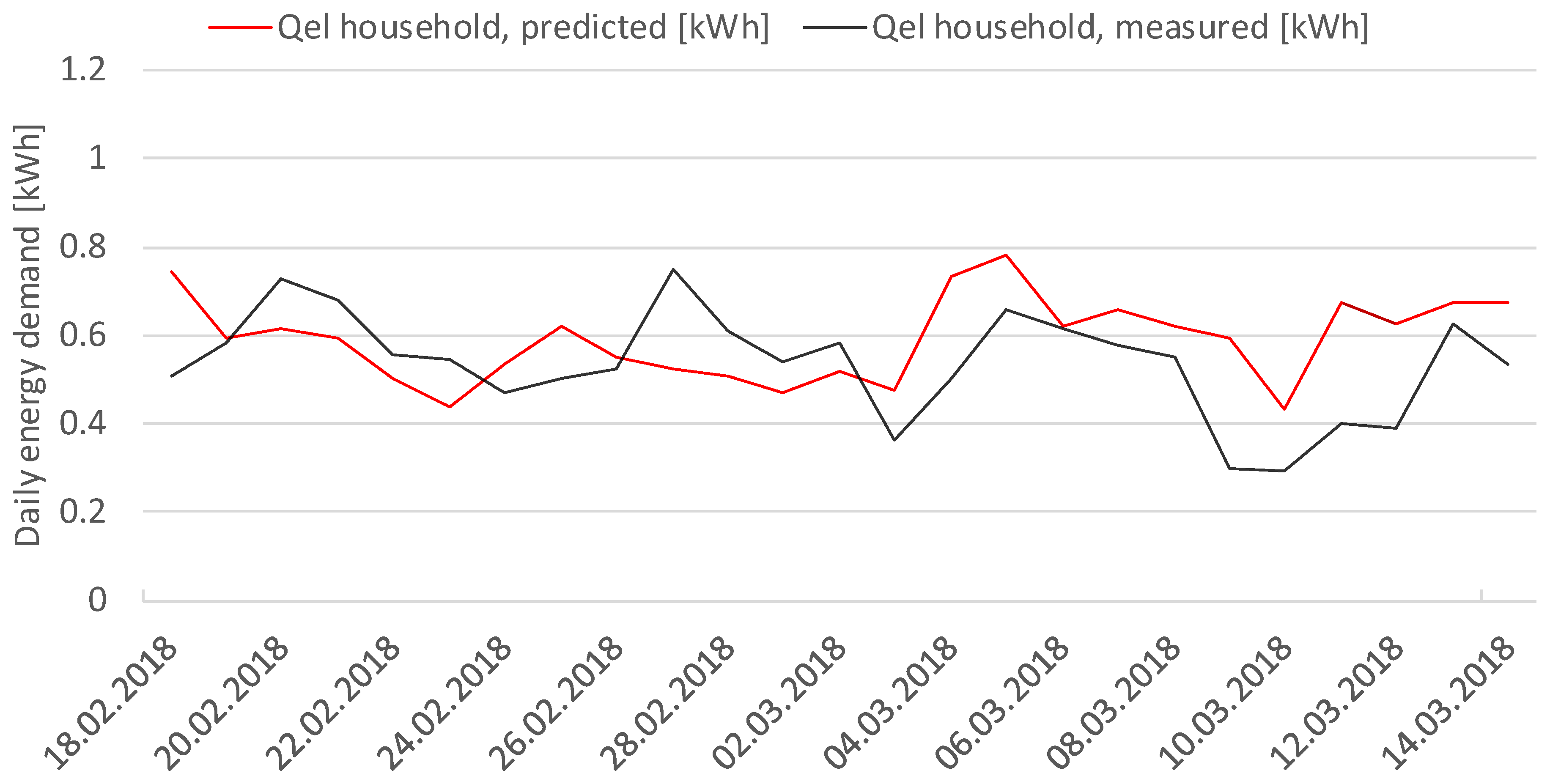
The daily requirement forecast (see Figure 20) also shows that the progression is sketched, but always shows a shift on the x and y axes. The hourly prediction by the DTR method (see Figure 21) shows that the model uses a kind of basic pattern for the prediction that is differently pronounced at the y-axis as well as at its shape, depending on the hour. The baseline in the model is much worse than that in the kNN method.

The daily prediction by the DTR method (see Figure 22) shows that the progression and proportions are similar to the actual demand, but there is a stronger shift on the x and y axes.

The prediction models with the kNN and DTR methods each have strengths and weaknesses, but the kNN model represents the data in the baseline and peak range more strongly. The problem with both models is that both can often not correctly position the demand peaks, which suggests that the models could achieve better predictive performance through better orientation.

The MAPE (see

Table 3. Evaluation results of kNN and DTR modeling. MAPE: mean absolute percentage error, MAE: percentage mean deviation.

Machine Learning Application	MAPE [%]	MAE [kWh]
kNN Hourly	108.67	0.27
kNN Daily	62.46	0.12
DTR Hourly	130.05	0.32
DTR Daily	80.51	0.16

) of the respective models roughly represents the results achieved in other studies with prediction models from the machine learning field [37].

With the results obtained so far, further methods from the field of machine learning are now being used to test their suitability as prediction models for the electrical energy demand of residential buildings. Furthermore, an analysis is carried out on how the dataset can be upgraded so that the procedures can better allocate peak demand. Here, for example, calendar information, such as school holidays, is implemented.

3.2. Optimization

For optimization purposes, it was decided to apply GA for several reasons. One is that they are, e.g., compared to PSO (particle swarm optimization), more suited for global search. Their suitability is also underlined by the fact that many studies with the aim to optimize HVAC systems rely on evolutionary and in specific on genetic algorithms [30].

In addition, compared to rule-based approaches, GA optimization is easier to be adapted for other use cases (flexible electricity tariffs, power markets, other system combinations) and not very sensitive to all events that are not covered within the rule-based approach, making it more adaptive and robust.

Within this work, for optimization purposes, a communication and control interface between the model in INSEL and Python—in particular the DEAP (Distributed Evolutionary Algorithms in Python, [43]) framework—was established. Using 24 h forecasts of ambient temperature and global radiation, optimized schedules for the following day’s heat pumps operation are created, addressing various optimization goals such as the highest self-consumption and lowest electricity costs in a flexible tariff model. Varying set point temperatures and switching on/off schedules of the heat pump were tested to charge buffer storages and also to increase the room temperature utilizing the building’s thermal mass to store energy. Optimization time steps are 5 minutes, taking into account the minimum operation times of heat pumps [44] and also allowing small steps of demand increase to find a better optimum. Model settling time and rebound effects are also assessed and reduced by a model parametrization using real values and a certain running time span before and after the 24 h optimization period. Regarding flexible electricity tariffs, a special methodology was applied according to [45] to generate ToU (Time of Use) tariffs that create more incentives for the end users.

In [46], it has been shown that varying the mutation and probability can reduce the amount of computational time by up to 50%. In [47], for a similar optimization goal, it was determined that a reduced number of simulation runs can be sufficient to find a nearby optimum since the forecast inaccuracy always brings an uncertainty, and therefore, an absolute optimum that applies to the reality cannot be found. Thus, a comprehensive iteration on the values of the algorithm operators (crossover probability, mutation probability) and its parameters (number of populations, number of generations) was carried out.

The algorithm’s target function e.g., for the optimization of self-consumption and/or a flexible electricity tariff, is the cumulated electricity cost and earnings over the prediction/optimization period described in the following equation.

$$M_{total}=Q_{el,pv\_grid}*m_{PV}-Q_{el,h_{grid}}*m_{h\_tariff}-Q_{el,HP\_grid}*m_{HP\_tariff}$$

(7)

with M_total [€] as the building’s daily monetary balance, m_PV [€/kWh] as the PV feed in the tariff, m_{h_tariff} [€/kWh] as the household electricity tariff, m_{HP_tariff} [€/kWh] as the heat pump electricity tariff, Q_{el,pv_grid} [kWh] as the daily amount of PV electricity to the grid, Q_{el,h_grid} [kWh] as the daily amount of household electricity from the grid, and Q_{el,HP_grid} [kWh] as the daily amount of heat pump electricity demand from the grid.

4. Results

4.1. Agrothermal Collector and Low-Temperature DHC Network

The economical assessment is done for an estimated collector and network lifetime of 40 years. The yearly rate for capital interest is assumed to be 3%, the inflation rate is assumed to be 1.5%, and the heat price increase is assumed to be 2%. The assumed cost and revenue are summarized in

Table 4. Cost used for the economical assessment.

Type	Cost
Installation of geothermal field [€/m2]	240,000
Installation of DHC network [€]	214,000
Subsidy [€]	246,600
Connection fee (180 €/kW, 136 kW connected) [€]	24,516
Annual heat revenue (7 €/kW monthly) [€/kW]	11,424

.

This leads to an assumed amortization time for the agrothermal collector and low-temperature DHC network of 27.5 years. It can be estimated that for the installment of further agrothermal collectors and the related low-temperature DHC network, the cost could drop as far as an equivalent heat price without subsidies [22].

4.2. Building-Side Heat End User Cost

For the end-user heat cost on the building side, the same assumptions are made as for the agrothermal collector and low-temperature DHC network regarding the yearly rate for capital interest, the inflation rate, and the heat price increase. The entire economical assessment is done for a 20-year component lifetime.

The specific investments for one individual building are listed in

Table 5. Investment costs within an individual building. DHW: domestic hot water.

Type	Investment Cost	Subsidy
Heat pump [€]	10,000	5000
Space heating buffer storage [€]	1300	500
DHW buffer storage [€]	400
Battery storage [€]	7000	7000
PV system incl. inverter [€]	17,000
DHC network connection costs [€]	3240
Heat distribution and transfer station [€]	9000

. It has to be noted that the 100% subsidy of the battery storage is granted within the project, whereas the subsidies for the heat pump and the space heating buffer storage are federal subsidies that can be claimed for all the newly constructed heat pump systems that fulfill the requirement within Germany.

Figure 23 shows that for the end user, the specific heat price including the costs and revenues of the whole system (e.g., also PV) is equal or better in comparison with other common heating solutions. This is partly the case because a subsidy for the battery storage is granted. However, even without a battery storage subsidy, the specific heat price would rise about 2.3 ct to 23.3 ct/kWh, which poses a competitive and sustainable solution. The fact that a natural gas grid is not available makes it in the case of Wüstenrot even more favorable. The detailed parameters of this calculation can be found in Appendix B (Figure A2 and Figure A3).

4.3. Optimization Parameters

For optimization 24 h in advance, 2500 calculation runs proved to be sufficient, resulting in 2:30 h of computation time on a dedicated off-the-shelf personal computer (Core I7-7700, 4 cores, 3.6 GHz). Thereby, in the simulation timespan, it was necessary to include the previous and following 3 h in addition to reducing the settling time at start up and to include a possible rebound effect. A crossover probability of 0.5 and a mutation probability of 0.5 have proven to be most efficient. In addition, with very little computational demand (e.g., 4–600 simulation runs), good results might randomly occur. For a further implementation on mini PCs, it is planned to change the thermal demand prediction to an RC model or a self-learning algorithm. It is estimated that this would reduce the computational demand by a factor of 10.

4.4. Self-Consumption

Simulation results, without taking into account the battery storage, suggest that through optimized heat pump operation for PV self-consumption, up to 50% of cost savings can be achieved during the course of one day under ideal conditions. Ideal conditions mean a low prediction inaccuracy, a good coincidence of demand and production by time and extent (amount of energy and peak power), and the available amount of thermal storage. The following figures show this case. Thereby, Figure 24A shows the normal PV yield and the corresponding heat pump operation as it would have occurred, and Figure 24B shows the optimized operation, shifting a significant part of the of the heat pump’s workload to the time of the maximum PV production. Figure 25 shows the corresponding development of the aggregated electricity costs without and with optimization. It can be seen that at first, during midday, the costs without optimization are cheaper since electricity is fed into the grid, and thus earnings are made by the assumed fixed price feed in the tariff. In contrast, during the later hours, this changes and the operation with optimization becomes significantly more favorable due to the discrepancy of feed in tariff costs (0.123 €/kWh in that case) and heat pump electricity costs (0.28 €/kWh in that case).

The hurdles for the optimization of self-consumption are that in summer (obviously) only DHW is prepared, and thus less demand exists, and also DHW storages tend to be too small dimensioned. In the transition period and in winter, there is a high heating demand, but the PV yield is significantly lower. In that time also, the PV system’s power output is not matching the heat pumps demand, resulting in additional electricity taken from the grid even at daily peak PV production. Installing larger buffer storages, matching the installed PV winter power output to the heat pump’s demand, and general conditions such as low or no PV feed in the tariff and high electricity tariff costs would results in higher monetary optimization benefits.

4.5. Flexible Electricity Tariffs

Flexible electricity tariffs can tend to include too small incentives and in some cases, not enough flexibility can be provided to gain an advantage from them. For example, directly applying the stock market trade price fluctuations to a tariff and thus giving this benefit to the end costumer unfortunately poses little incentive, as it can be seen in

Table 6. German electricity tariff composition (March 2019) [48,49,50].

Type	Specific Cost
EEG (renewable energy sources act) reallocation charge	64.05 €/MWh
CHP (combined heat and power) surcharge	2.80 €/MWh
§19 StromNEV-reallocation	3.05 €/MWh
Offshore apportionment of liability	4.16 €/MWh
Reallocation charge for switchable loads	0.05 €/MWh
Electricity grid usage charge	73.90 €/MWh
Concession charge	16.60 €/MWh
Electricity tax	20.50 €/MWh
Procurement (av. spot market price EPEX Oct 2018–March 2019)	46.79 €/MWh
Profit margin of reseller	20.00 €/MWh
VAT (value added tax)	47.86 €/MWh
Total	299.76 €/MWh

and Figure 26, since within the composition of the end-user electricity price, procurement and thus the volatile part plays a minor role (16%). Further adaptions are needed to make flexible electricity tariffs more inciting. Thereby, one option can be ToU (Time of Use) tariffs or CPP (critical peak pricing) tariffs based on either a dynamic FIT (Feed-In Tariff) surcharge or a dynamic network fee such as that developed and described in [45]. This approach is also applied to this work to generate a theoretical tariff for estimating its benefits with and without heat pump optimization.

The following Figure 27A shows a flexible electricity tariff included in the heat pump’s daily operation; Figure 27B shows the same situation, but with an optimization algorithm applied to the heat pump’s operation. Figure 28 shows the corresponding development of the aggregated electricity costs with and without optimization. Compared to the previous optimization of PV self-consumption, the achieved cost reduction of 17% is significantly lower. This can be explained by the fact that the thermal flexibility potential in that case was not sufficient. Therefore, the size of the thermal buffer storages is not only relevant because of their maximum thermal storage capacity in kWh, but also due to the temperature levels at which the heat pump is operating. This affects the COP and thus can reduce the monetary benefit of the optimization significantly.

4.6. Power Markets

Simulation-based studies focusing on a single building in the Plus-Energy settlement have so far shown a significant potential regarding a participation in aFRR (automatic frequency restoration reserve) market under certain conditions where 48% of the heat pump’s electricity demand could be provided by aFRR within a yearly energy balance. In that case, 11% more electricity was needed to provide the demanded heat due to a lower COP and higher thermal losses because of the higher operating temperatures. Thereby, PV self-consumption was only reduced from 36% to 34%. Thereby, the main hurdles were the very short activation durations from the aFRR market that lead to problems in heat pump cycling. This could be addressed by cluster management and by a change in the legal framework. [51,52]

5. Discussion

Within this work, a Plus-Energy settlement with 23 residential buildings equipped with decentralized heat pumps and PV systems in the German municipality of Wüstenrot was introduced. The buildings are connected to a low-temperature DHC network and a novel agrothermal heat source: a geothermal collector at depths of around 2 m that allows heat withdrawal and agriculture usage at the same time. A broad overview of the lessons learned, monitoring results, and the application of DR and DSM on the building level combined with a simulation-based prediction and optimization approach was given.

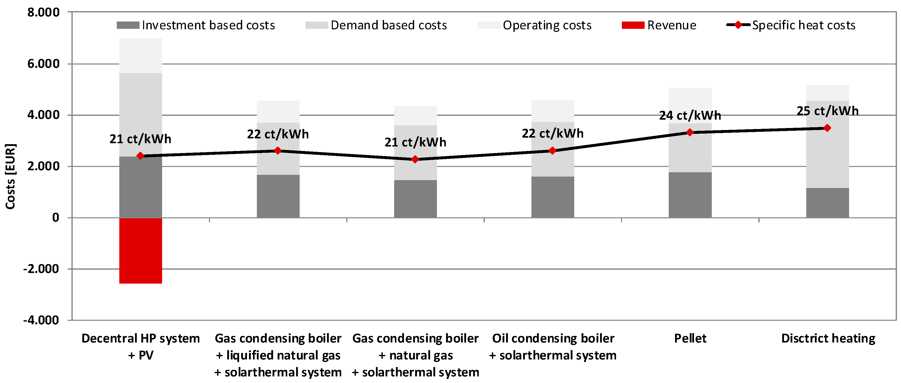
Investigations of the low-temperature DHC network with decentralized heat pumps showed that heating and cooling energy can be produced efficiently at an average annual heat pump COP of approximately 4. With the subsidies granted within the research project, a competitive heat price of 0.21 €/kWh for the end user was achieved. It is expected that with progressing maturity of the technology, competitive heat prices can also be reached without subsidies.

The geothermal monitoring showed that there is a significant impact on the specific heat yield by groundwater resulting in more than 100 kWh/m² due to high moisture and the energy transfer generated by the groundwater. This leads to a reduction of the collector field size. In the case of the Plus-Energy settlement in Wüstenrot, a low-temperature DHC network also has proven to be very suitable since it is situated in a less dense, more rural area with highly efficient buildings and available wider open areas for collector installment.

Within the settlement, the agrothermal collector, and the low-temperature DHC network, a comprehensive monitoring system was installed. Especially within six of the buildings, data of all the relevant thermal and electrical energy flows are gathered in great detail, and the heat pumps are controllable. For monitoring and control, mainly ModBus TCP and ModBus RTU protocols are used. Data is collected in a cloud-based MySQL database and accessed by a dedicated monitoring solution.

On the building level, an approach for the prediction of building demand and production as well as optimization of heat pump operation was developed to increase self-consumption, apply flexible electricity tariffs, and also participate in power markets.

Thereby, the individual thermal load forecast and the behavior of the building systems was realized via white box simulation models, whereas the prediction of household electricity and DHW demand was done by an algorithm based on DTR, kNN, and k-means clustering, constantly trained by previous measured data. The prediction and optimization was realized in the simulation environment INSEL and in Python. The implementation was so far carried out for only one building but will in the future include six buildings of the Plus-Energy settlement.

Validation has shown an MAPE of the heat pump system of 22.8% (daily basis), an MAPE of the PV system of 22.1% (hourly basis), and MAPE values of the household electricity prediction of 47.0% (hourly basis) and 28.1% (daily basis). Thereby, it was found that user behavior poses the biggest inaccuracy and problems while weather forecast inaccuracy is acceptable, especially for thermal demand predictions.

For optimization purposes of the heat pump’s operation, it was decided to apply GA because of its suitability for this specific problem e.g., compared to PSO or rule-based heuristic approaches. Optimization for 24 h in advance with 2500 simulation runs resulted in approximately 2.5 h of computation time, which was mainly due to the white box thermal demand prediction. This optimization time could be reduced by a factor of 10, utilizing an RC (resistance capacity) model for thermal demand prediction, but would also result in more prediction inaccuracy.

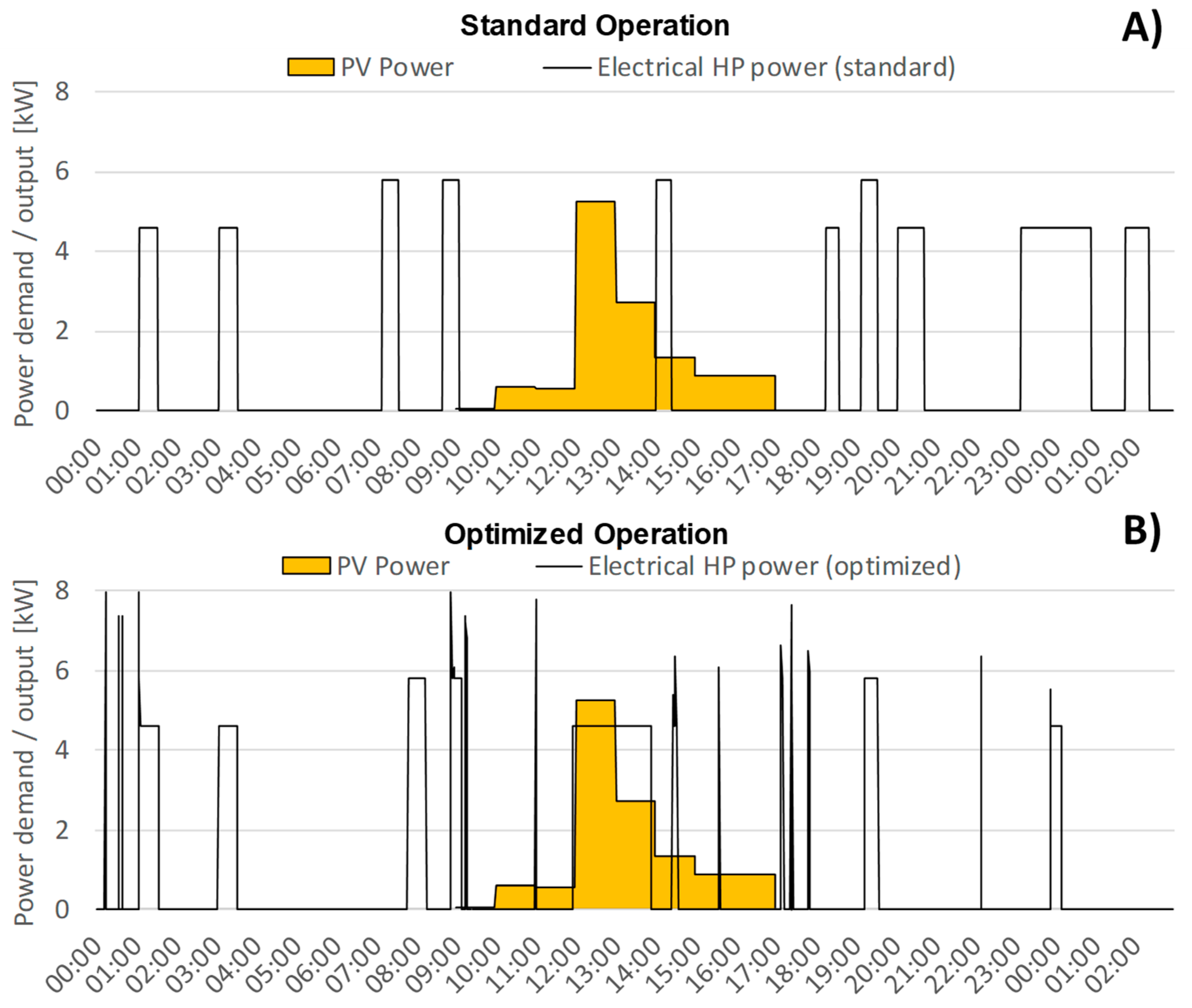
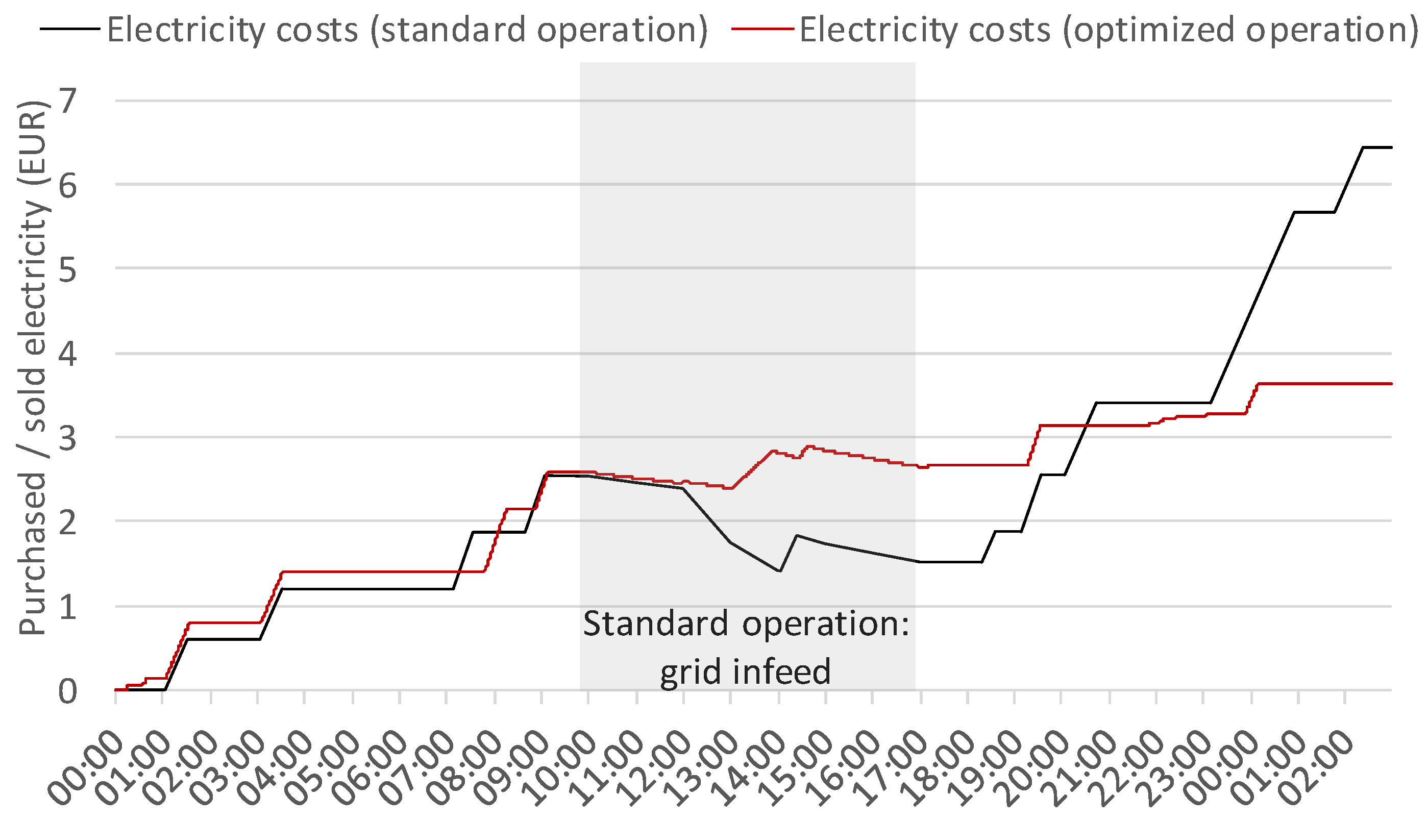
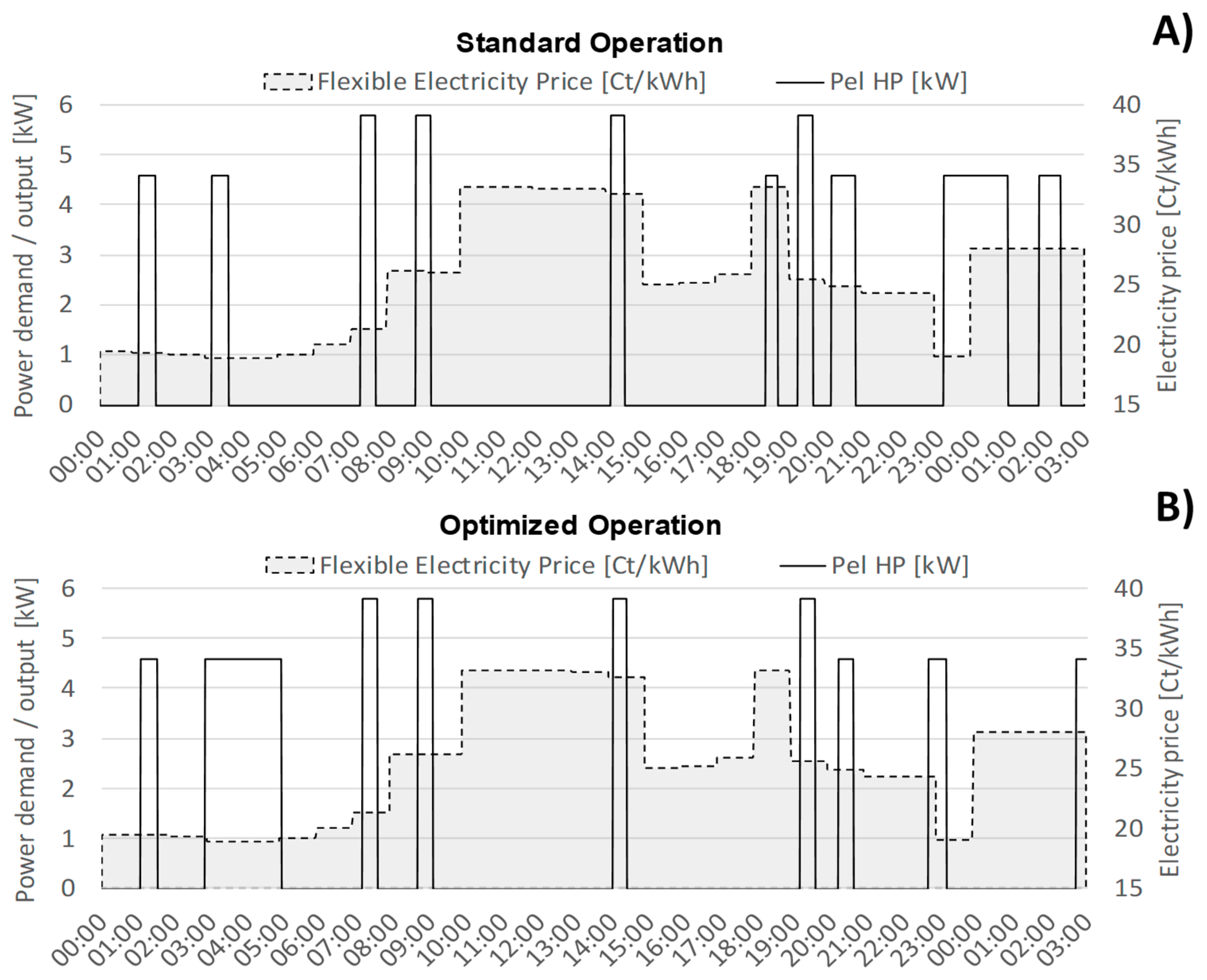
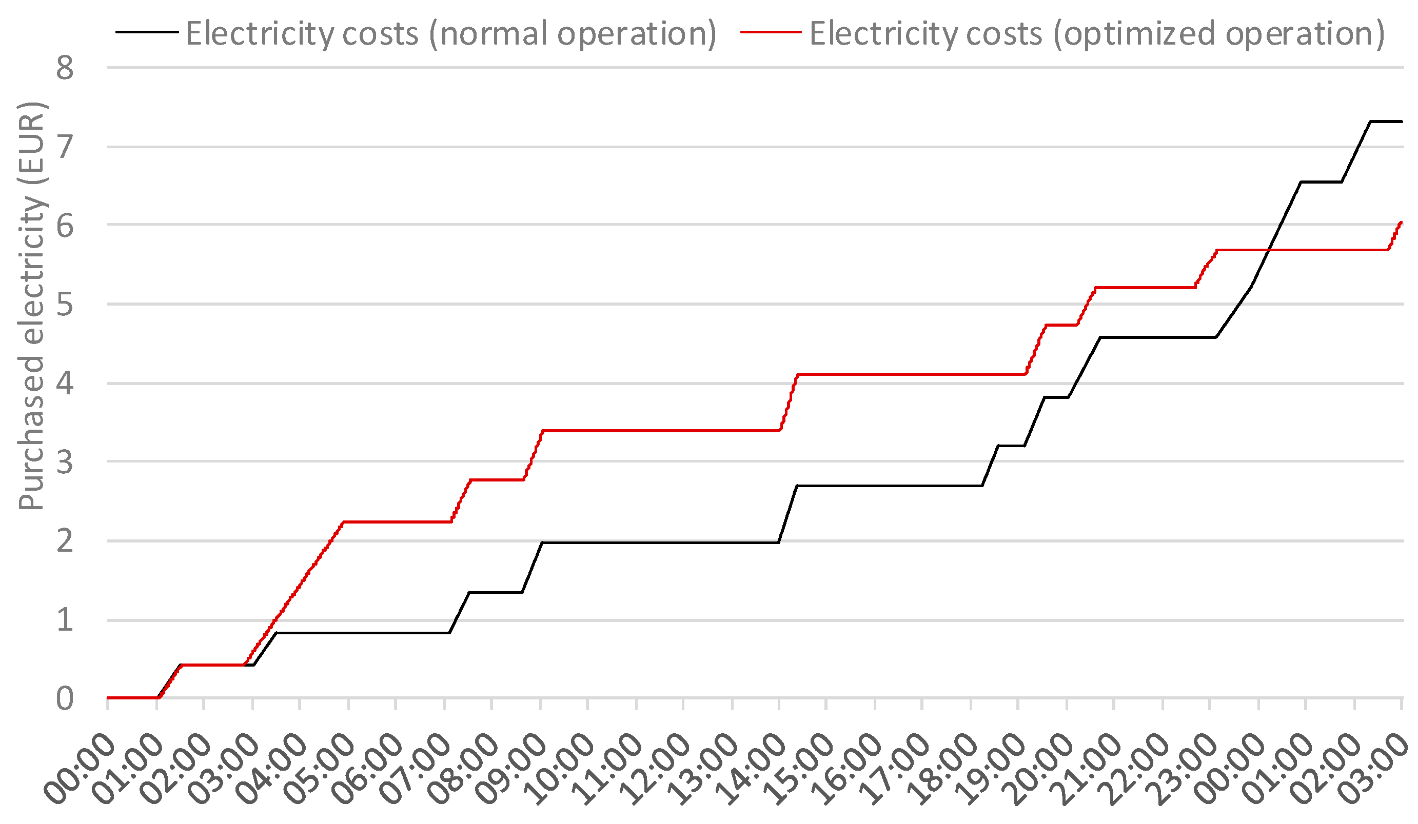
Simulation results for one building have shown for PV self-consumption that through optimized heat pump operation and overcharging of the thermal buffer storages, up to 50% of cost savings could be achieved during the course of one day under ideal conditions. It has been found that the hurdles for the optimization of self-consumption are that in summer only DHW is prepared and thus less demand exists, and also that DHW storages tend to be too small. In addition, that in winter and the transition time the PV system’s power output dos not match the heat pump’s demand results in additional electricity taken from the grid. It was recommended to install larger thermal buffer storages and to match the installed PV winter power output to the heat pump’s demand. In addition, general conditions such as low or no PV feed in the tariff and high electricity tariff costs together with no installed battery storage are ideal cases for this optimization approach.

In addition, the utilization of flexible electricity tariffs was examined on the building level. Thereby, it is important that the tariffs show enough monetary variability whereas e.g., forwarding the fluctuations of the spot market to the end user would show too little incentive. Even with adequate flexible tariffs, enough thermal flexibility and thus larger thermal buffer storages and/or a higher comfort tolerance of the buildings occupants are required. The size of the thermal buffer storages is thereby not only relevant because of their maximum thermal capacity, but also because of the temperature levels at which the heat pump is operating. Simulation results have shown that even with enough storage capacity available, the higher temperatures reduced the heat pump’s COP to such a degree that the monetary benefit of the optimization was reduced.

Based on the here described work, simulation-based studies were also published previously [51,52] addressing the potential of a participation in aFRR (secondary reserve) markets. Thereby, for a single building of the Plus-Energy settlement with battery storage, up to 48% of the heat pump’s electricity demand could be provided by aFRR within a yearly balance, only reducing PV self-consumption from 36% to 34%. Thereby, the main problems were the very short activation durations from the aFRR market that lead to problems in heat pump cycling, which could be addressed by cluster management and by a change in the legal framework.

Within the ongoing research project Sim4Blocks, in the future, building optimization for six buildings shall be implemented. Further, it is planned to operate those buildings aggregated as a single virtual power plant also including activation calls by an aggregator.

The limitations of this work are that only a very specific system combination—an agrothermal collector with a low-temperature DHC network on the district level, and on the building level mainly single family houses with high energy efficiency standard, decentralized heat pumps and PV systems—is investigated, which can limit the transferability of the results. In addition, agrothermal collectors are limited to areas with sufficient space; even in Wüstenrot, as a rural municipality, it has proven to be difficult to find adequate areas. In addition, part of the presented results are simulation-based, and they still have to be proven in real operation.