A Comparison of Different District Integration for a Distributed Generation System for Heating and Cooling in an Urban Area


Abstract
1. Introduction
- research focusing on the optimization of the operation of energy systems, ranging from the optimization of a single component, to the operation of the overall DG system;
- research dealing with the optimization of the system synthesis; and
- research focusing on synthesis, design and operation optimization.
- almost all models rely on linear programming or mixed integer linear programming (MILP). However, some approaches based on meta-heuristics (simulated annealing, genetic algorithms, etc.) have been proposed, but they present some difficulties concerning the determination of search parameters and the judgment about optimality [11,12,13].
- the research normally focus only on specific targets: operation or synthesis optimization, economic and/or environmental optimization, unit or district heating network (DHN) optimization, etc.
2. MILP Model
2.1. Decision Variables and Constraints
- binary variables: they represent the existence/absence of each component and the operation status (on/off) of each component in each time interval. There are other additional binary variables which do not represent any physical quantity, added to linearize some relations; and
- continuous variables: they represent the size of components, the size of pipelines, the load of components in each time interval, the energy content of the storages and the connection flows.
- components;
- district heating and cooling network;
- thermal storage; and
- energy balances.
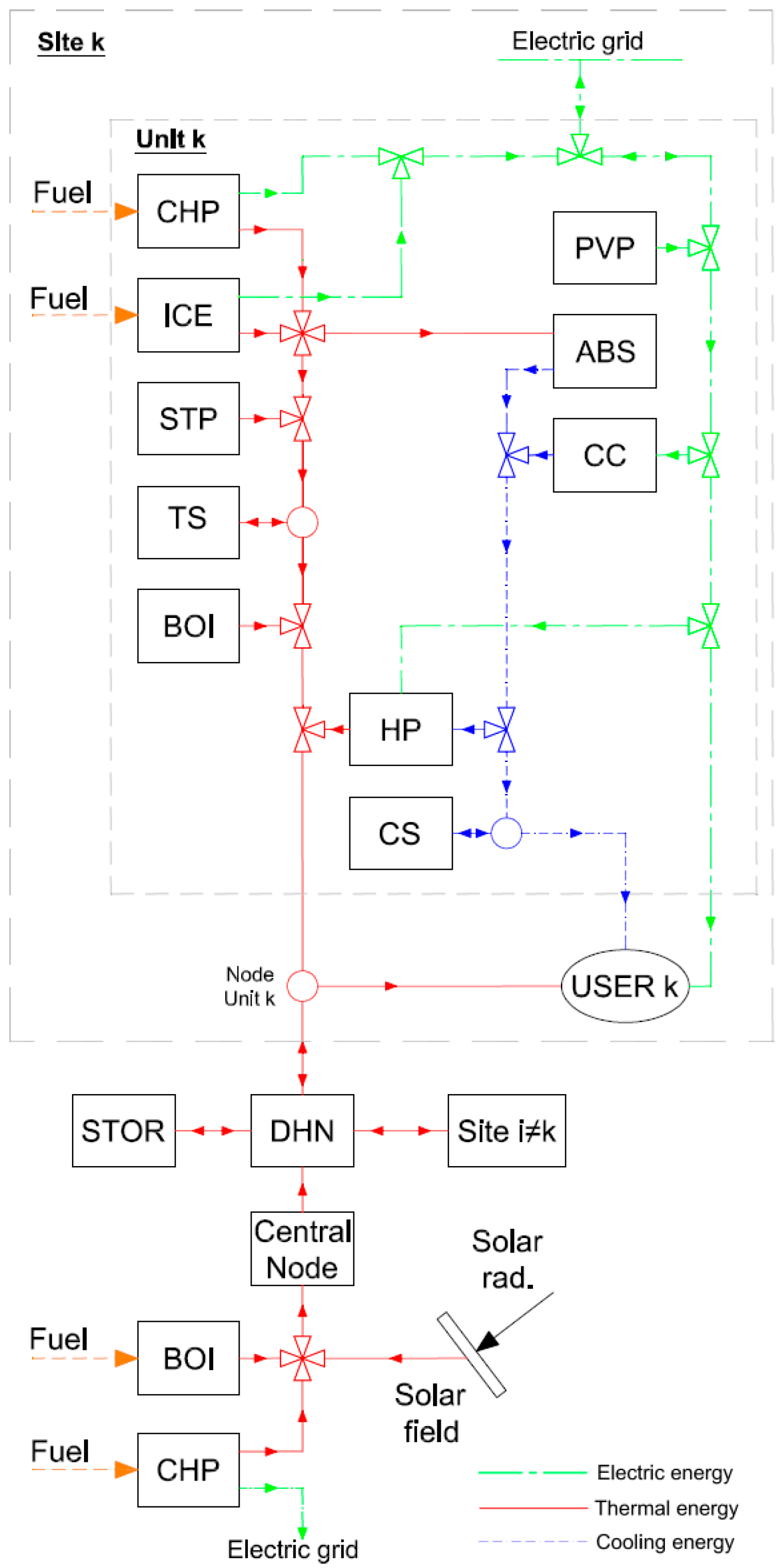
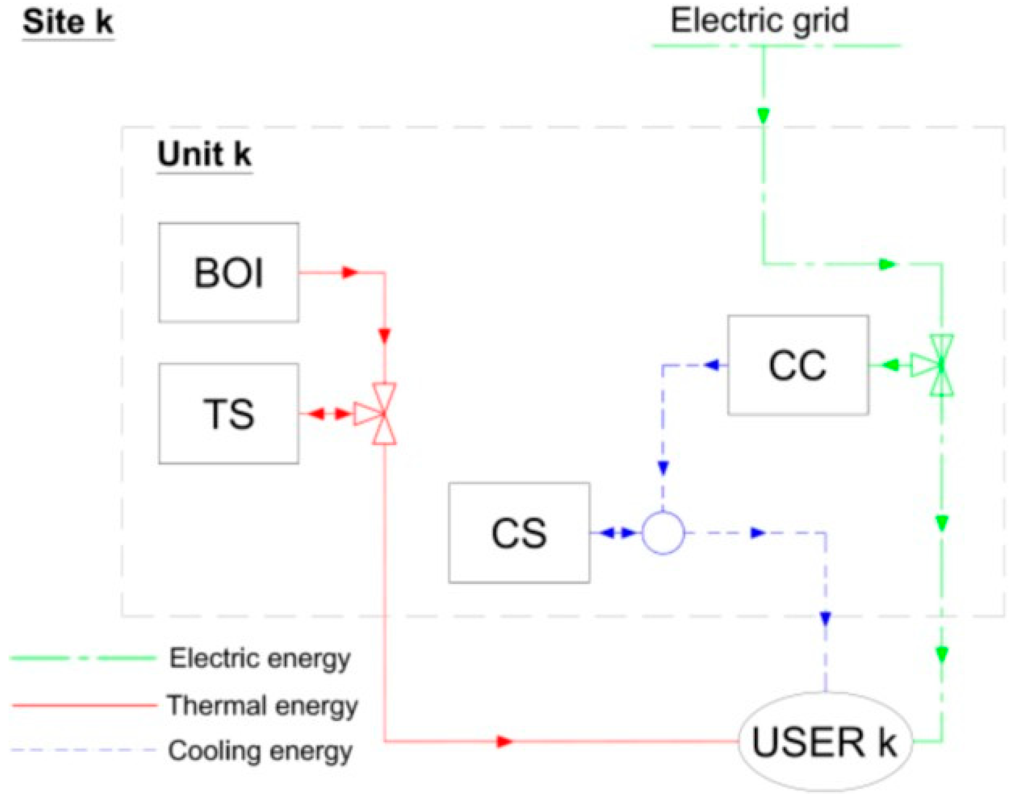
2.2. Components
2.3. District Heating and Cooling Network
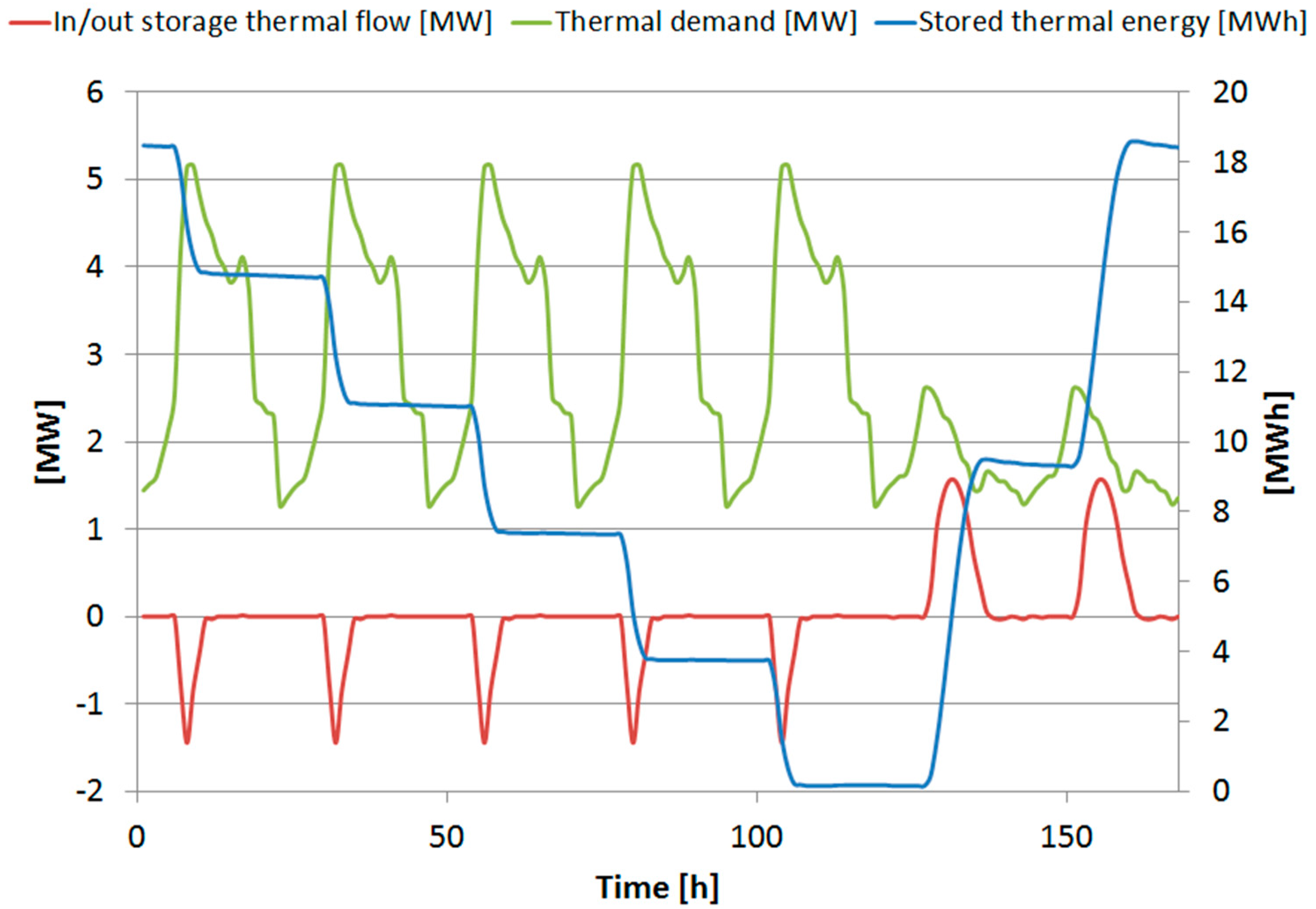
2.4. Thermal Storage
2.5. Energy Balances
2.6. Objective Functions
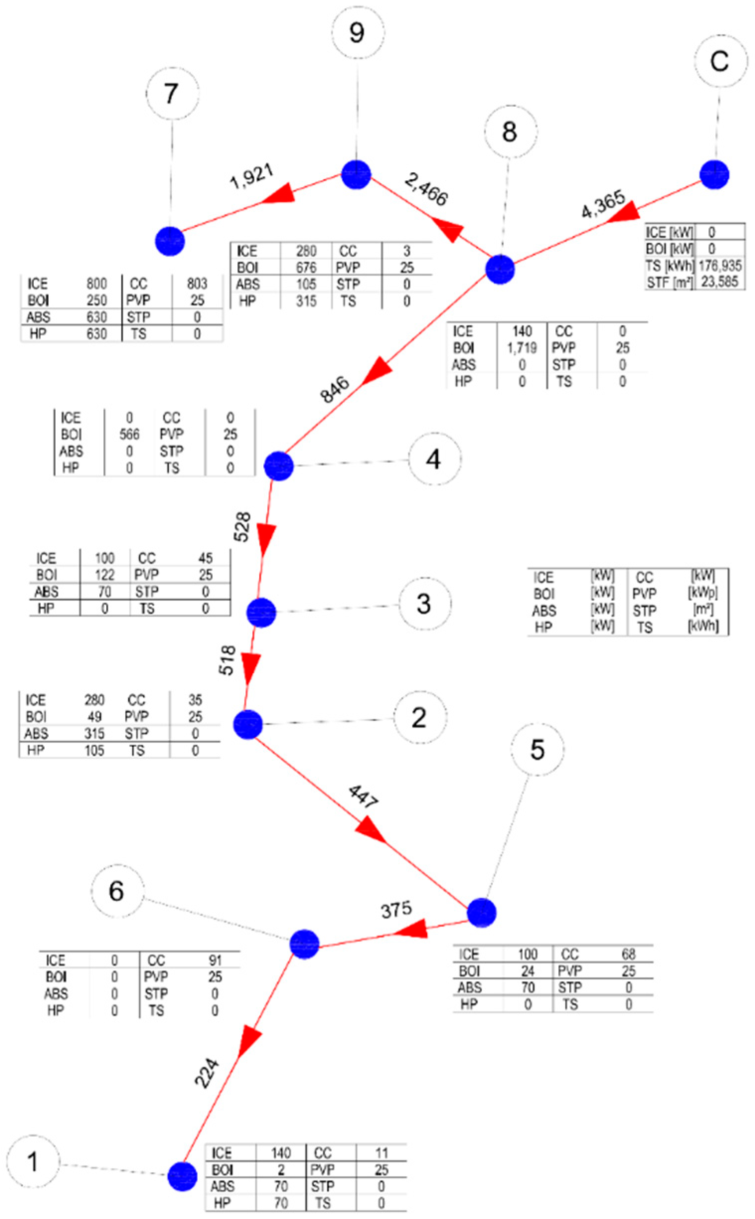
3. Case Study
- layout of the roads which connect the buildings;
- position of the underground utilities (waterworks, sanitation, gas network, etc.); and
- location of the boiler rooms of the buildings.
- natural gas detaxation for cogeneration use; and
- renewable energy production incentives.
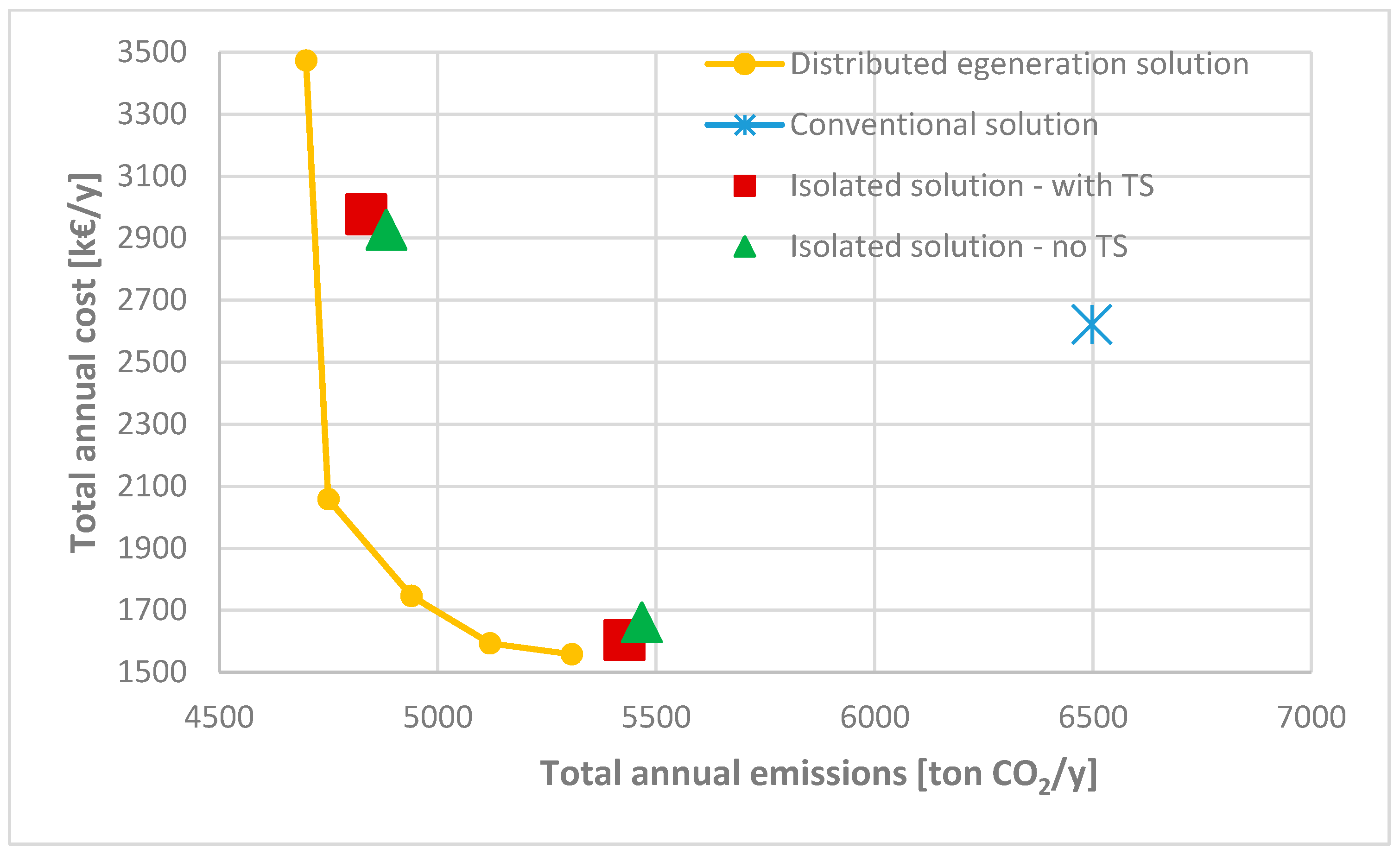
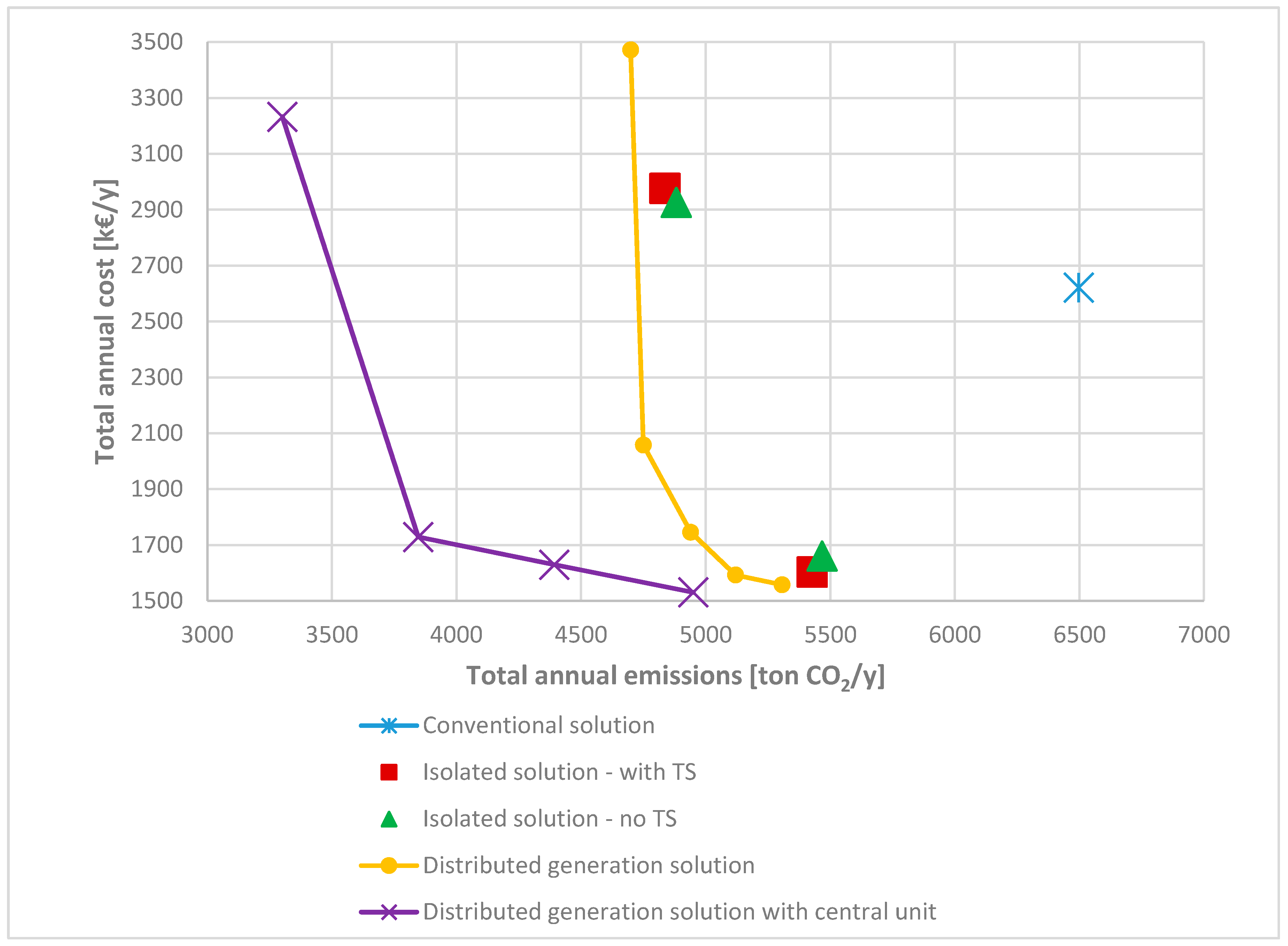
4. Results of the Optimizations
- conventional solution;
- isolated solution;
- distributed generation solution without central unit and district cooling network;
- distributed generation solution with central unit but without cooling network; and
- complete distributed generation solution.
4.1. Conventional Solution
4.2. Isolated Solution
4.3. Distributed Generation Solution
4.4. Distributed Generation Solution Integrated with the Central Solar System
4.5. Complete Distributed Generation Solution
5. Conclusions
- conventional solution;
- isolated solution;
- distributed generation solution without central unit and district cooling network;
- distributed generation solution with central unit but without cooling network; and
- complete distributed generation solution.
Supplementary Materials
Author Contributions
Funding
Conflicts of Interest
Nomenclature
| δt | Thermal losses percentage |
| ∆t | Difference between outlet and inlet temperatures (K) |
| ηboi,c | Central BOI efficiency |
| ψboi,c | Additional variable for the centralized BOI |
| ρp | Medium density (Kg/m3) |
| ξice,c | Additional variable for the centralized Internal Combustion Engine (ICE) |
| Ap | Diameter of the pipeline (m2) |
| c | Central unit |
| Cabs | Cold produced by the Absorption Chiller (ABS) (kWh) |
| cabs | ABS investment cost (e) |
| cboi | BOI investment cost (e) |
| cboi,f | BOI fixed investment cost (e) |
| cboi,v | BOI variable investment cost (e/kW) |
| Ccc | Cold produced by the Compression Chiller (CC) (kWh) |
| Cdem | User cooling demand (kWh) |
| cel,bgt | Electricity cost (e/kWh) |
| cel,inc | Photo-voltaic panels (PV panels) incentive (e/kWh) |
| cel,sol | Electricity income (e/kWh) |
| cfue,boi | BOI fuel cost (e/kWh) |
| cfue,chp | Combined Cooling Heat and Power (CHP) fuel cost (e/kWh) |
| cfue,ice,c | Central ICE fuel cost (e/kWh) |
| chp | HP investment cost (e) |
| Chp | Cold produced by the HP (kWh) |
| cice | ICE investment cost (e) |
| cice,f | ICE fixed investment cost (e) |
| cice,v | ICE variable investment cost (e/kW) |
| cinv | Investment annual cost (e/y) |
| cinv,c | Central unit annual investment cost (e/y) |
| cinv,u | Site annual investment cost (e/y) |
| cman | Maintenance annual cost (e/y) |
| cmgt | Micro Gas Turbine (MGT) investment cost (e) |
| cnet | DHCN annual investment cost (e/y) |
| cnet,f,c | Fixed cost of the DHCN pipeline (e/m) |
| cnet,v | Variable cost of the DHCN pipeline (e/kW · m) |
| cnet,v,c | Variable cost of the central DHN pipeline (e/kW · m) |
| cope | Operating annual cost (e/y) |
| cope,c | Central unit annual operation cost (e/y) |
| cope,u | Unit annual operation cost (e/y) |
| cp | Specific heat(Kj/kg K) |
| cpvp | PV panels investment cost (e/m) |
| cstp | Solar thermal panels (ST panels) investment cost (e/m2) |
| cstp,c | Central ST panels investment cost (e/m2) |
| ctot | Total annual cost (e/y) |
| Cts | Cooling energy storage input (kWh) |
| cts | Thermal Storage (TS) investment cost (e/kWh) |
| cts,c | Central TS investment cost (e/kWh) |
| d | Generic day |
| Ebgt | Electricity bought from the network (kWh) |
| Ecc | Electricity required by the CC (kWh) |
| Ehp,c | Electricity required by the HP when producing cold (kWh) |
| Edem | User electricity demand (kWh) |
| Ehp,h | Electricity required by the HP when producing heat (kWh) |
| Ehp | Electricity required by the HP (kWh) |
| Eice | Electricity produced by the ICE (kWh) |
| Eice,c | Electricity produced by the centralized ICE (kWh) |
| Eice,lim | ICE operation limits (kW) |
| emel | Electricity carbon intensity (kgCO2/kWh) |
| emf,boi | BOI fuel carbon intensity (kgCO2/kWh) |
| emf,cen | Central CHP fuel carbon intensity (kgCO2/kWh) |
| emf,chp | CHP fuel carbon intensity (kgCO2/kWh) |
| Emgt | Electricity produced by the MGT (kWh) |
| emlim | Emission limit in the s-constrained optimization (kgCO2/kWh) |
| emtot | Total annual CO2 emissions (kg) |
| Epvp | Electricity produced by the PV panels (kWh) |
| Esol | Electricity sold to the network (kWh) |
| fabs | ABS amortization factor (y−1) |
| Fboi | Fuel required by the BOI (kWh) |
| fboi | BOI amortization factor (y−1) |
| Fboi,c | Fuel required by the central BOI (kWh) |
| fcc | CC amortization factor (y−1) |
| fhp | HP amortization factor (y−1) |
| Fice | Fuel required by the ICE (kWh) |
| fice | ICE amortization factor (y−1) |
| Fice,c | Fuel required by the centralized ICE (kWh) |
| Fmgt | Fuel required by the MGT (kWh) |
| fmgt | MGT amortization factor (y−1) |
| fnet | DHCN amortization factor (y−1) |
| fpvp | PV panels amortization factor (y−1) |
| fstp | ST panels amortization factor (y−1) |
| fts | TS amortization factor (y−1) |
| h | Generic hour |
| Habs | Heat required by the ABS (kWh) |
| Hboi | Heat produced by the BOI (kWh) |
| Hboi,c | Heat produced by the central BOI (kWh) |
| Hboi,lim,c | Centralized BOI operation limits (kW) |
| Hdem | User thermal demand (kWh) |
| Hhp | Heat produced by the HP (kWh) |
| Hice | Heat produced by the ICE (kWh) |
| Hice,c | Heat produced by the centralized ICE (kWh) |
| Hmgt | Heat produced by the MGT (kWh) |
| Hnet | Thermal energy transferred through the pipeline (kWh) |
| Hnet,c | Thermal energy transferred through the pipeline of the central DHN (kWh) |
| Hnet,lim | Size limits of the pipelines (kWh) |
| Hstp | Solar panel thermal production |
| Hstp,c | Centralized solar field thermal production |
| Hts | Thermal energy storage input (kWh) |
| Hts,c | Thermal energy storage input (kWh) |
| j | Generic component |
| k | Generic site/user |
| Kfice | ICE Performance curve linearization coefficient |
| Kfice,c | Centralized ICE Performance curve linearization coefficient |
| Khice | ICE Performance curve linearization coefficient |
| Khice,c | Central ICE performance curve linearization coefficient |
| Khp | HP Performance curve linearization coefficient |
| Klos,ts | Percentage thermal loss coefficient |
| Kpv | Unitary PV production |
| Kstp | Unitary solar thermal production |
| lp | Length of the pipeline (m) |
| m | Generic month |
| Oboi,c | Central BOI operation (binary) |
| Ohp,c | HP cold operation (binary) |
| Ohp,h | HP heat operation (binary) |
| Oice | ICE operation (binary) |
| Oice,c | Centralized ICE operation (binary) |
| pt | Pipeline thermal loss per unit length (km−1) |
| pt,c | Pipeline thermal loss per unit length of the central DHN pipeline (km−1) |
| Heat transferred by a DHCN pipeline (kWh) | |
| Qts | Thermal energy stored in a thermal storage (kWh) |
| s | Generic week |
| Sboi | BOI size (kW) |
| Sboi,c | Central BOI size (kW) |
| Sboi,lim,c | Central BOI size limits (kW) |
| Scc | CC size (kW) |
| SC,net | Size of the cooling pipeline (kW) |
| Scs | Cooling storage size (kWh) |
| SH,net | Size of the thermal pipeline (kW) |
| SH,net,c | Size of the central DHN pipeline (kW) |
| Shp,lim | HP operation limits (kW) |
| Sice,c | Centralized ICE size |
| Sice,lim,c | Centralized ICE size limits (kW) |
| Spvp | Size of the PV panels equipment |
| Sstp | Size of the solar equipment |
| Sstp,c | Size of the central solar field |
| Sts | Thermal storage size (kWh) |
| Sts,c | Central thermal storage size (kWh) |
| u, v | Generic unit |
| vp | Velocity of the medium inside the pipeline (m/s) |
| Vts | Thermal storage volume (m3) |
| wgt | Time interval weight |
| Xabs | ABS existence (binary) |
| Xboi,c | Central BOI existence (binary) |
| Xcp | Existence of the cooling pipeline (binary) |
| Xhp | HP existence (binary) |
| Xice | ICE existence (binary) |
| Xice,c | Centralized ICE existence (binary) |
| Xmgt | MGT existence (binary) |
| Xnet | Existence of a network pipeline (binary) |
| Xnet,c | Existence of the central DHN (binary) |
| Xtp | Existence of the thermal pipeline (binary) |
Acronims
| ABS | Absorption chiller |
| BOI | Boiler |
| CC | Compression chiller |
| CHP | Combined cooling heat and power |
| COP | Coefficient of performance |
| CS | Cooling storage |
| DCN | District cooling network |
| DG | Distributed generation |
| DHCN | District heating and cooling network |
| DHN | District heating network |
| HP | Heat pump |
| ICE | Internal combustion engine |
| MGT | Micro gas turbine |
| MILP | Mixed integer linear programming |
| PV panels | Photovoltaic panels |
| ST field | Solar thermal field |
| ST panels | Solar thermal panels |
| TS | Thermal storage |
References
- Ban˜os, R.; Manzano-Agugliaro, F.; Montoya, F.G.; Gil, C.; Alcayde, A.; G’omez, J. Optimization methods applied to renewable and sustainable energy: A review. Renew. Sustain. Energy Rev. 2011, 15, 1753–1766. [Google Scholar] [CrossRef]
- Henning, D. Energy System Optimization Applied to Local Swedish Utilities. Ph.D. Thesis, Linkopings University, Linköping, Sweden, 1992. [Google Scholar]
- Henning, D. MODEST—An energy system optimisation model applicable to local utilities and countries. Energy 1997, 22, 1135–1150. [Google Scholar] [CrossRef]
- Curti, V.; von Spakovsky, M.R.; Favrat, D. An environomic approach for the modeling and optimization of a district heating network based on centralized and decentralized heat pumps, cogeneration and/or gas furnace. Part I: Methodology. Int. J. Therm. Sci. 2000, 39, 721–730. [Google Scholar] [CrossRef]
- Yokoyama, R.; Hasegawa, Y.; Ito, K. A MILP decomposition approach to large scale optimization in structural design of energy supply systems. Energy Convers. Manag. 2002, 43, 771–790. [Google Scholar] [CrossRef]
- Karlsson, M. The MIND method: A decision support for optimization of industrial energy systems principles and case studies. Appl. Energy 2011, 88, 577–589. [Google Scholar] [CrossRef][Green Version]
- Ortiga, J.; Bruno, J.C.; Coronas, A.; Grossman, I.E. Review of optimization models for the design of polygeneration systems in district heating and cooling networks. In ESCAPE17; Elsevier: Amsterdam, The Netherlands, 2007; pp. 1–6. [Google Scholar]
- Pohekar, S.D.; Ramachandran, M. Application of multi-criteria decision making to sustainable energy planning—A review. Renew. Sustain. Energy Rev. 2004, 8, 365–381. [Google Scholar] [CrossRef]
- Bazmi, A.A.; Zahedi, G. Sustainable energy systems: Role of optimization modeling techniques in power generation and supply—A review. Renew. Sustain. Energy Rev. 2011, 15, 3480–3500. [Google Scholar] [CrossRef]
- Liew, P.Y.; Theo, W.L.; Alwi, S.R.W.; Lim, J.S.; Manan, Z.A.; Klemeš, J.J.; Varbanov, P.S. Total Site Heat Integration planning and design for industrial, urban and renewable systems. Renew. Sustain. Energy Rev. 2017, 68, 964–985. [Google Scholar] [CrossRef]
- Munoz, J.R. Optimization Strategies for the Synthesis/Design of Highly Coupled, Highly Dynamic Energy Systems. Ph.D. Thesis, Virginia Polytechnic Institute and State University, Blacksburg, VA, USA, 2000. [Google Scholar]
- Li, H.; Nalim, R.; Haldi, P.A. Thermal-economic optimization of a distributed multi- generation energy system—A case study of Beijing. Appl. Therm. Eng. 2006, 26, 709–719. [Google Scholar] [CrossRef]
- Kavvadias, K.C.; Maroulis, Z.B. Multi-objective optimization of a trigeneration plant. Energy Policy 2010, 38, 945–954. [Google Scholar] [CrossRef]
- Chinese, D.; Meneghetti, A. Optimisation models for decision support in the development of biomass-based industrial district-heating networks in Italy. Appl. Energy 2005, 82, 228–254. [Google Scholar] [CrossRef]
- Söderman, J.; Pettersson, F. Structural and operational optimisation of distributed energy systems. Appl. Therm. Eng. 2006, 26, 1400–1408. [Google Scholar] [CrossRef]
- Pavicevic, M.; Novosel, T.; Puksec, T.; Duic, N. Hourly optimization and sizing of district heating systems considering building refurbishment—Case study for the city of Zagreb. Energy 2017, 137, 1264–1276. [Google Scholar] [CrossRef]
- Pérez-Mora, N.; Lazzeroni, P.; Martínez-Moll, V.; Repetto, M. Optimal management of a complex DHC plant. Energy Convers. Manag. 2017, 145, 386–397. [Google Scholar] [CrossRef]
- Ameri, M.; Besharati, Z. Optimal design and operation of district heating and cooling networkswith CCHP systems in a residential complex. Energy Build. 2016, 110, 135–148. [Google Scholar] [CrossRef]
- Ren, H.; Zhou, W.; Nakagami, K.; Gao, W.; Wu, Q. Multi-objective optimization for the operation of distributed energy systems considering economic and environmental aspects. Appl. Energy 2010, 87, 3642–3651. [Google Scholar] [CrossRef]
- Carvalho, M. Thermoeconomic and Environmenal Analyses for the Synthesis of Poly- Generation Systems in the Residential-Commercial Sector. Ph.D. Thesis, University of Zaragoza, Zaragoza, Spain, 2011. [Google Scholar]
- Ito, K.; Yokoyama, R. A revised decomposition method for MILP problems and its application to operational planning of thermal storage systems. J. Energy Resour. Technol. 1996, 118, 227–235. [Google Scholar]
- Ito, K.; Akagi, S. An optimal planning method for a marine heat and power generation plant by considering its operational problem. Int. J. Energy Res. 1986, 10, 75–85. [Google Scholar] [CrossRef]
- Ito, K.; Yokoyama, R. Optimal operational planning of cogeneration system with thermal storage by the decomposition method. J. Energy Resour. Technol. 1995, 117, 337–343. [Google Scholar]
- Silva, V.V.; Fleming, P.J.; Sugimoto, J.; Yokoyama, R. Multiobjective optimization using variable complexity modelling for control system design. Appl. Soft Comput. 2008, 8, 392–401. [Google Scholar] [CrossRef]
- Lazzarin, R.; Noro, M. Local or district heating by natural gas: Which is better from energetic, environmental and economic point of views? Appl. Therm. Eng. 2006, 26, 244–250. [Google Scholar] [CrossRef]
- Dobersek, D.; Goricanec, D. Optimisation of tree path pipe network with non- linear optimisation method. Appl. Therm. Eng. 2009, 29, 1584–1591. [Google Scholar] [CrossRef]
- Verda, V.; Baccino, G.; Sciacovelli, A.; Russo, S.L. Impact of district heating and groundwater heat pump systems on the primary energy needs in urban areas. Appl. Therm. Eng. 2012, 40, 18–26. [Google Scholar] [CrossRef]
- Rezaie, B.; Rosen, M.A. District heating and cooling: Review of technology and potential enhancements. Appl. Energy 2011, 93, 2–10. [Google Scholar] [CrossRef]
- Tveit, T.; Savola, T.; Gebremedhin, A.; Fogelholm, C. Multi-period MINLP model for optimising operation and structural changes to CHP plants in district heating networks with long-term thermal storage. Energy Convers. Manag. 2009, 50, 639–647. [Google Scholar] [CrossRef]
- Badyda, K.; Bujalski, W.; Milewski, J.; Warcho, M. Heat accumulator in large district heating systems—Simulation and optimisation. In Proceedings of the ASME Turbo Expo 2010, Glasgow, UK, 14–18 June 2010; pp. 1–6. [Google Scholar]
- Domínguez-Muñoz, F.; Cejudo-López, J.M.; Carrillo-Andrés, A.; Gallardo-Salazar, M. Selection of typical demand days for CHP optimization. Energy Build. 2011, 43, 3036–3043. [Google Scholar] [CrossRef]
- Ortiga, J.; Bruno, J.C.; Coronas, A. Selection of typical days for the characterisation of energy demand in cogeneration and trigeneration optimisation models for buildings. Energy Convers. Manag. 2011, 52, 1934–1942. [Google Scholar] [CrossRef]
- International Energy Agency. Co2 Emissions from Fuel Combustion; IEA Publications: Paris, France, 2011. [Google Scholar]
- Marler, R.T.; Arora, J.S. Survey of multi-objective optimization methods for engineering. Struct. Multidiscip. Optim. 2004, 26, 369–395. [Google Scholar] [CrossRef]
- Italian Parlament. D.lgs. 79/99 Electricity and Gas Italian Market Liberalization; Italian Parliament: Roma, Italy, 1999.
- Italian Parlament. D.Lgs 70/07 Implementation of the EU Directive 2008/4/Ce; Italian Parliament: Roma, Italy, 2007.
- Italian Parlament. Decree July 5th, 2012: Quinto Conto Energia; Italian Parliament: Roma, Italy, 2012.


| ELECTRIC | HEATING | COOLING | ||||
|---|---|---|---|---|---|---|
| USERS | Year Dem. | Peak Power | Year Dem. | Peak Power | Year Dem. | Peak Power |
| (MWh) | (kWe) | (MWh) | (kWt) | (MWh) | (kWc) | |
| Town Hall | 346,640 | 189 | 692,720 | 410 | 148,712 | 150 |
| Theatre | 852,208 | 270 | 908,648 | 655 | 457,688 | 458 |
| Library | 492,240 | 110 | 587,608 | 296 | 112,364 | 115 |
| Primary School | 73,808 | 54 | 979,468 | 591 | 0 | 0 |
| Retirement Home | 489,048 | 101 | 739,956 | 246 | 207,568 | 138 |
| Archive | 82,516 | 36 | 429,604 | 238 | 78,652 | 91 |
| Hospital | 3,284,416 | 628 | 7,884,141 | 1847 | 1,445,612 | 2087 |
| Secondary School | 303,668 | 148 | 2,301,980 | 2084 | 0 | 0 |
| Swimming Pool | 1,043,572 | 315 | 2,794,580 | 1425 | 297,416 | 435 |
| Total | 6,968,116 | 1717 | 17,318,705 | 7017 | 2,748,012 | 3048 |
| User Peak Power sum | 1851 | 7792 | 3474 | |||
| Equipment | Unit 1 | Unit 2 | Unit 3 | Unit 4 | Unit 5 | Unit 6 | Unit 7 | Unit 8 | Unit 9 |
|---|---|---|---|---|---|---|---|---|---|
| MGT | 65 | 100 | 30 | 30 | 30 | 30 | 200 | 65 | 100 |
| ICE | 70 | 140 | 50 | 50 | 50 | 50 | 200 | 70 | 140 |
| ABS | 70 | 105 | 35 | 35 | 35 | 35 | 105 | 70 | 105 |
| HP | 70 | 105 | 35 | 35 | 35 | 35 | 105 | 70 | 105 |
| User | 1 | 2 | 3 | 4 | 5 | 6 | 7 | 8 | 9 |
|---|---|---|---|---|---|---|---|---|---|
| Electric Peak (kW) | 189 | 270 | 110 | 54 | 101 | 36 | 628 | 148 | 315 |
| Thermal Peak (kW) | 410 | 655 | 296 | 591 | 246 | 238 | 1847 | 2084 | 1425 |
| Cooling Peak (kW) | 150 | 458 | 115 | 0 | 138 | 91 | 2087 | 0 | 435 |
| Boiler (kW) | 294 | 479 | 217 | 418 | 205 | 179 | 1623 | 1673 | 1153 |
| Comp. Chiller (kW) | 150 | 458 | 115 | 0 | 138 | 91 | 2087 | 0 | 435 |
| Thermal storage (kW) | 544 | 375 | 312 | 766 | 173 | 298 | 690 | 2251 | 1564 |
| User | 1 | 2 | 3 | 4 | 5 | 6 | 7 | 8 | 9 | Total |
|---|---|---|---|---|---|---|---|---|---|---|
| Natural gas (k€/y) | 44 | 58 | 37 | 62 | 47 | 27 | 498 | 146 | 177 | 1096 |
| Electricity cost (k€/y) | 67 | 171 | 90 | 13 | 95 | 18 | 640 | 52 | 194 | 1340 |
| Operating cost (k€/y) | 111 | 228 | 127 | 75 | 142 | 46 | 1138 | 198 | 371 | 2437 |
| Maintenance cost (k€/y) | 1 | 2 | 1 | 1 | 1 | 1 | 11 | 2 | 3 | 23 |
| Total investment cost (k€/y) | 58 | 141 | 43 | 33 | 47 | 35 | 597 | 127 | 188 | 1267 |
| Annual investment cost (k€/y) | 7 | 18 | 6 | 4 | 6 | 4 | 77 | 16 | 24 | 163 |
| Total annual cost (k€/y) | 120 | 248 | 134 | 80 | 149 | 51 | 1226 | 216 | 399 | 2622 |
| Electricity emission (t/y) | 141 | 358 | 189 | 26 | 199 | 39 | 1341 | 108 | 407 | 2807 |
| Natural gas emission (t/y) | 148 | 194 | 125 | 209 | 158 | 92 | 1677 | 492 | 596 | 3691 |
| Total annual emission (t/y) | 289 | 551 | 314 | 236 | 356 | 130 | 3018 | 600 | 1003 | 6497 |
| User | 1 | 2 | 3 | 4 | 5 | 6 | 7 | 8 | 9 | Total |
|---|---|---|---|---|---|---|---|---|---|---|
| Bought Electricity (MWh) | 396 | 1005 | 530 | 74 | 558 | 109 | 3766 | 304 | 1143 | 7884 |
| Electricity user demand (MWh) | 347 | 852 | 492 | 74 | 489 | 83 | 3284 | 304 | 1044 | 6968 |
| Electricity required by CC (MWh) | 50 | 153 | 37 | 0 | 69 | 26 | 482 | 0 | 99 | 916 |
| Heat produced by BOI (MWh) | 696 | 911 | 590 | 984 | 741 | 432 | 7888 | 2312 | 2802 | 17,357 |
| Thermal user demand (MWh) | 693 | 909 | 588 | 979 | 740 | 430 | 7884 | 2302 | 2795 | 17,319 |
| Wasted heat (MWh) | 0 | 0 | 0 | 0 | 0 | 0 | 0 | 0 | 0 | 0 |
| Cooling energy by CC (MWh) | 149 | 458 | 112 | 0 | 208 | 79 | 1446 | 0 | 297 | 2748 |
| Cooling energy user demand (MWh) | 149 | 458 | 112 | 0 | 208 | 79 | 1446 | 0 | 297 | 2748 |
| Wasted cooling energy (MWh) | 0 | 0 | 0 | 0 | 0 | 0 | 0 | 0 | 0 | 0 |
| Economic Optimization | Environmental Optimization | ||||
|---|---|---|---|---|---|
| Conventional Solution | Isolated Solution without TS | Isolated Solution | Isolated Solution without TS | Isolated Solution | |
| ICE (kW) | 0 | 2820 | 2840 | 4920 | 4920 |
| MGT (kW) | 0 | 0 | 0 | 3900 | 3900 |
| BOI (kW) | 6241 | 2145 | 984 | 609 | 431 |
| ABS (kW) | 0 | 840 | 735 | 3570 | 3570 |
| HP (kW) | 0 | 1750 | 980 | 3570 | 3570 |
| CC (kW) | 3474 | 1274 | 1763 | 1948 | 2008 |
| PV panels (kW) | 0 | 225 | 225 | 45 | 0 |
| ST panels (m2) | 0 | 0 | 0 | 1438 | 1800 |
| TS (kWh) | 6973 | 0 | 15,016 | 0 | 36,000 |
| CS (kW) | 0 | 0 | 0 | 0 | 36,000 |
| Economic Optimization | Environmental Optimization | ||||
|---|---|---|---|---|---|
| Conventional Solution | Isolated Solution without TS | Isolated Solution | Isolated Solution without TS | Isolated Solution | |
| CHP natural gas cost (k€/y) | 0 | 1458 | 1561 | 624 | 600 |
| BOI natural gas cost (k€/y) | 1096 | 67 | 50 | 13 | 2 |
| Buoght electricity cost (k€/y) | 1340 | 29 | 28 | 1216 | 1257 |
| Sold electricity income (k€/y) | 0 | 365 | 490 | 138 | 140 |
| Photovolatic incentive (k€/y) | 0 | 68 | 68 | 16 | 0 |
| Operating cost (k€/y) | 2437 | 1121 | 1081 | 1699 | 1720 |
| Maintenance cost (k€/y) | 23 | 120 | 128 | 53 | 52 |
| Total investment cost (k€/y) | 1267 | 4288 | 4021 | 12,138 | 12,518 |
| Annual investment cost (k€/y) | 163 | 421 | 395 | 1175 | 1206 |
| Total annual cost (k€/y) | 2622 | 1661 | 1604 | 2927 | 2977 |
| Reduction wrt conv. solution | 36.7% | 38.8% | −11.6% | −13.5% | |
| Electricity emissions (t/y) | 2807 | 61 | 59 | 2545 | 2633 |
| Sold electricity emissions (t/y) | 0 | 1363 | 1806 | 508 | 499 |
| Natural gas emissions (t/y) | 3691 | 6769 | 7173 | 2844 | 2701 |
| Total annual emissions (t/y) | 6497 | 5467 | 5427 | 4882 | 4836 |
| Reduction wrt conv. solution | 15.9% | 16.5% | 24.9% | 25.6% | |
| Economic Optimization | Environmental Optimization | ||||
|---|---|---|---|---|---|
| Conventional Solution | Isolated Solution without TS | Isolated Solution | Isolated Solution without TS | Isolated Solution | |
| ICE electricity | 0 | 11,563 | 12,455 | 4599 | 4591 |
| MGT electricity | 0 | 0 | 0 | 331 | 175 |
| PV panels electricity | 0 | 239 | 239 | 48 | 0 |
| Bought electricity | 7884 | 173 | 166 | 7150 | 7395 |
| Electric user demand | 6968 | 6968 | 6968 | 6968 | 6968 |
| CC electricity | 916 | 137 | 191 | 398 | 394 |
| HP electricity | 0 | 1042 | 628 | 3337 | 3399 |
| Sold electricity | 0 | 3828 | 5073 | 1426 | 1,4012 |
| ICE thermal energy | 0 | 16,906 | 18,133 | 6603 | 6628 |
| MGT thermal energy | 0 | 0 | 0 | 566 | 299 |
| BOI thermal energy | 17,357 | 1064 | 787 | 205 | 36 |
| HP thermal energy | 0 | 2103 | 946 | 9279 | 9419 |
| ST panels thermal energy | 0 | 0 | 0 | 1108 | 1387 |
| Thermal user demand | 17,319 | 17,319 | 17,319 | 17,319 | 17,319 |
| ABS thermal energy | 0 | 1733 | 1604 | 290 | 131 |
| Wasted thermal energy | 0 | 1022 | 399 | 152 | 92 |
| CC cooling energy | 2748 | 410 | 574 | 1194 | 1182 |
| ABS cooling energy | 0 | 1127 | 1055 | 163 | 79 |
| HP cooling energy | 0 | 1213 | 1121 | 1392 | 1488 |
| Cooling energy demand | 2748 | 2748 | 2748 | 2748 | 2748 |
| Wasted cooling energy | 0 | 2 | 1 | 0 | 0 |
| Environmental Opt. | 90% Env. Opt. | 60% Env. Opt. | 30% Env. Opt. | Economic Opt. | |
|---|---|---|---|---|---|
| DHN pipes (n°) | 18 | 13 | 9 | 7 | 7 |
| ICE (kW) | 1920 | 2190 | 2290 | 2590 | 28,403,900 |
| MGT (kW) | 3900 | 0 | 0 | 0 | 0 |
| BOI (kW) | 502 | 0 | 0 | 0 | 0 |
| ABS (kW) | 3570 | 0 | 0 | 595 | 770 |
| HP (kW) | 3570 | 2590 | 2380 | 1715 | 1050 |
| CC (kW) | 1593 | 1682 | 1759 | 1620 | 1656 |
| PV panels (kWp) | 0 | 0 | 134 | 225 | 225 |
| ST panels (m2) | 1800 | 1800 | 734 | 0 | 0 |
| TS (kWh) | 36,000 | 6316 | 8553 | 12,337 | 15,017 |
| CS (kWh) | 36,000 | 0 | 0 | 0 | 0 |
| Environmental Optimization | 90% Env. Optimization. | 60% Env. Optimization. | 30% Env. Optimization. | Economic Optimization. | |
|---|---|---|---|---|---|
| CHP natural gas cost (k€/y) | 389 | 643 | 994 | 1296 | 1614 |
| BOI natural gas cost (k€/y) | 0 | 0 | 0 | 0 | 0 |
| Buoght electricity cost (k€/y) | 1603 | 1030 | 446 | 130 | 21 |
| Sold electricity income (k€/y) | 76 | 82 | 126 | 264 | 539 |
| Photovolatic incentive (k€/y) | 0 | 0 | 30 | 58 | 67 |
| Operating cost (k€/y) | 1917 | 1591 | 1284 | 1105 | 1028 |
| Maintenance cost (k€/y) | 37 | 57 | 84 | 107 | 132 |
| Annual investment cost (k€/y) | 1519 | 410 | 378 | 381 | 397 |
| Total investment cost (k€/y) | 17,422 | 4403 | 3968 | 4050 | 4178 |
| Total annual cost (k€/y) | 3472 | 2058 | 1746 | 1593 | 1558 |
| Reduction wrt conv. solution | −32.44% | 21.52% | 33.42% | 39.23% | 40.59% |
| Electricity emissions (t/y) | 3358 | 2157 | 934 | 273 | 44 |
| Sold electricity emissions (t/y) | 269 | 292 | 456 | 972 | 1981 |
| Natural gas emissions (t/y) | 1710 | 2885 | 4461 | 5818 | 7244 |
| Total annual emissions (t/y) | 4699 | 4750 | 4940 | 5120 | 5307 |
| Reduction wrt conv. solution | 27.68% | 26.89% | 23.97% | 21.20% | 18.33% |
| Environmental Optimization | 90% Env. Optimization | 60% Env. Optimization | 30% Env. Optimization | Economic Optimization | |
|---|---|---|---|---|---|
| ICE electricity | 3131 | 5190 | 8014 | 10,341 | 12,933 |
| MGT electricity | 0 | 0 | 0 | 0 | 0 |
| PV panels electricity | 0 | 0 | 141 | 239 | 239 |
| Bought electricity | 9431 | 6060 | 2625 | 767 | 123 |
| Electric user demand | 6968 | 6968 | 6968 | 6968 | 6968 |
| CC electricity | 217 | 230 | 266 | 180 | 231 |
| HP electricity | 4617 | 3232 | 2266 | 1560 | 532 |
| Sold electricity | 760 | 820 | 1281 | 2729 | 5565 |
| ICE thermal energy | 4619 | 7468 | 11,510 | 15,022 | 18,742 |
| MGT thermal energy | 0 | 0 | 0 | 0 | 0 |
| BOI thermal energy | 0 | 0 | 0 | 0 | 3 |
| HP thermal energy | 11,581 | 8663 | 5406 | 3450 | 834 |
| ST panels thermal energy | 1387 | 1387 | 566 | 0 | 0 |
| Thermal user demand | 17,319 | 17,319 | 17,319 | 17,319 | 17,319 |
| ABS thermal energy | 0 | 0 | 0 | 809 | 1704 |
| Wasted thermal energy | 0 | 0 | 0 | 0 | 9 |
| CC cooling energy | 652 | 689 | 797 | 540 | 692 |
| ABS cooling energy | 0 | 0 | 0 | 523 | 1140 |
| HP cooling energy | 2096 | 2059 | 1951 | 1686 | 917 |
| Cooling user demand | 2748 | 2748 | 2748 | 2748 | 2748 |
| Wasted cooling energy | 0 | 0 | 0 | 0 | 1 |
| Environmental | 70% Env. | 30% Env. | Economic | |
|---|---|---|---|---|
| Opt. | Opt. | Opt. | Opt. | |
| DHN pipes [n°] | 14 | 8 | 7 | 7 |
| Central pipe size (kW) | 7500 | 6323 | 3579 | 1907 |
| ICE (kW) | 4920 | 1840 | 2380 | 2500 |
| MGT (kW) | 0 | 0 | 0 | 0 |
| BOI (kW) | 3480 | 3408 | 2730 | 2023 |
| ABS (kW) | 3570 | 1260 | 1155 | 1085 |
| HP (kW) | 3570 | 1120 | 1225 | 1155 |
| CC (kW) | 1584 | 1056 | 1053 | 1233 |
| PV panels (kWp) | 225 | 225 | 225 | 225 |
| ST panels (m2) | 0 | 0 | 0 | 0 |
| TS (kWh) | 0 | 0 | 2315 | 5134 |
| CS (kWh) | 0 | 0 | 0 | 0 |
| Central ICE (kW) | 0 | 0 | 0 | 0 |
| Central BOI (kW) | 0 | 0 | 0 | 0 |
| ST field (m2) | 27,736 | 23,585 | 19,013 | 8035 |
| Central TS (kWh) | 400,000 | 173,935 | 41,855 | 19,025 |
| Environmental | 70% Env. | 30% Env. | Economic | |
|---|---|---|---|---|
| Opt. | Opt. | Opt. | Opt. | |
| CHP natural gas cost (k€/y) | 86 | 741 | 1059 | 1339 |
| BOI natural gas cost (k€/y) | 1 | 10 | 9 | 33 |
| Buoght electricity cost (k€/y) | 1482 | 451 | 221 | 32 |
| Sold electricity income (k€/y) | 30 | 125 | 234 | 373 |
| Photovolatic cost (k€/y) | 75 | 53 | 55 | 66 |
| Operating cost (k€/y) | 1464 | 1025 | 1000 | 965 |
| Maintenance cost (k€/y) | 10 | 63 | 88 | 113 |
| Total investment cost [k€] | 22,314 | 8248 | 6368 | 5359 |
| Annual investment cost (k€/y) | 1760 | 705 | 569 | 453 |
| Total annual cost (k€/y) | 3233 | 1792 | 1657 | 1531 |
| Reduction wrt conv. solution | −22.32% | 31.64% | 36.89% | 41.61% |
| Electricity emissions (t/y) | 3104 | 945 | 463 | 67 |
| Sold electricity emissions (t/y) | 190 | 461 | 856 | 1385 |
| Natural gas emissions (t/y) | 388 | 3362 | 4748 | 6268 |
| Total annual emissions (t/y) | 3301 | 3846 | 4392 | 4950 |
| Reduction wrt conv. solution | 49.20% | 40.80% | 32.41% | 23.81% |
| Environmental | 70% Env. | 30% Env. | Economic | |
|---|---|---|---|---|
| Opt. | Opt. | Opt. | Opt. | |
| ICE electricity | 693 | 5957 | 8482 | 10,956 |
| MGT electricity | 0 | 0 | 0 | 0 |
| PV panels electricity | 239 | 239 | 239 | 239 |
| Bought electricity | 8718 | 2656 | 1302 | 188 |
| Electric user demand | 6968 | 6968 | 6968 | 6968 |
| CC electricity | 209 | 137 | 121 | 162 |
| HP electricity | 1938 | 453 | 529 | 363 |
| Sold electricity | 534 | 1294 | 2404 | 3889 |
| ICE thermal energy | 1024 | 8547 | 12,284 | 15,979 |
| MGT thermal energy | 0 | 0 | 0 | 0 |
| BOI thermal energy | 11 | 161 | 146 | 529 |
| HP thermal energy | 3991 | 675 | 866 | 497 |
| ST panels thermal energy | 20,931 | 17,880 | 14,651 | 6191 |
| Thermal user demand | 17,319 | 17,319 | 17,319 | 17,319 |
| ABS thermal energy | 0 | 2316 | 2336 | 2341 |
| Wasted thermal energy | 7850 | 6918 | 8018 | 2571 |
| CC cooling energy | 626 | 410 | 364 | 487 |
| ABS cooling energy | 0 | 1521 | 1522 | 1549 |
| HP cooling energy | 2122 | 820 | 872 | 717 |
| Cooling user demand | 2748 | 2748 | 2748 | 2748 |
| Wasted cooling energy | 0 | 3 | 10 | 4 |
| Environmental | 70% Env. | 30% Env. | Economic | |
|---|---|---|---|---|
| Optimization | Opt. | Opt. | Optimization | |
| DHN pipes (n°) | 14 | 8 | 7 | 7 |
| DCN pipes (n°) | 7 | 4 | 3 | 3 |
| Central pipe size (kW) | 7500 | 4980 | 4118 | 1922 |
| ICE (kW) | 4920 | 1840 | 2270 | 2380 |
| MGT (kW) | 0 | 0 | 0 | 0 |
| BOI (kW) | 12 | 1954 | 1406 | 1252 |
| ABS (kW) | 3570 | 1435 | 1190 | 1120 |
| HP (kW) | 3570 | 1890 | 1680 | 1680 |
| CC (kW) | 778 | 250 | 174 | 306 |
| PV panels (kWp) | 225 | 225 | 225 | 225 |
| ST panels (m2) | 0 | 0 | 0 | 0 |
| TS (kWh) | 0 | 0 | 2176 | 4939 |
| CS (kWh) | 0 | 0 | 0 | 0 |
| Central ICE | 0 | 0 | 0 | 0 |
| Central BOI | 0 | 0 | 0 | 0 |
| ST field (m2) | 22,736 | 21,764 | 17,664 | 8710 |
| Central TS (kWh) | 400,000 | 169,926 | 30,980 | 20,366 |
| Environmental Optimization | 70% Env. Opt. | 30% Env. Opt. | Economic Optimization | |
|---|---|---|---|---|
| CHP natural gas cost (k€/y) | 202 | 757 | 1026 | 1242 |
| BOI natural gas cost (k€/y) | 0 | 7 | 4 | 33 |
| Buoght electricity cost (k€/y) | 1474 | 486 | 218 | 38 |
| Sold electricity income (k€/y) | 126 | 153 | 266 | 340 |
| Photovolatic incentive (k€/y) | 75 | 53 | 56 | 66 |
| Operating cost (k€/y) | 1475 | 1045 | 926 | 908 |
| Maintenance cost (k€/y) | 10 | 60 | 88 | 107 |
| Total investment cost (k€/y) | 24,806 | 8114 | 6909 | 5219 |
| Annual investment cost (k€/y) | 1611 | 680 | 592 | 466 |
| Total annual cost (k€/y) | 3095 | 1785 | 1606 | 1481 |
| Reduction wrt conv. solution | −18.05% | 31.93% | 38.75% | 43.50% |
| Electricity emissions (t/y) | 3087 | 1018 | 457 | 80 |
| Sold electricity emissions (t/y) | 197 | 453 | 864 | 1157 |
| Natural gas emissions (t/y) | 403 | 3262 | 4769 | 5974 |
| Total annual emissions (t/y) | 3292 | 3827 | 4362 | 4897 |
| Reduction wrt conv. solution | 49.33% | 41.10% | 32.87% | 24.63% |
| Environmental | 70% Env. | 30% Env. | Economic | |
|---|---|---|---|---|
| Optimization | Opt. | Opt. | Optimization | |
| ICE electricity | 726 | 5807 | 8510 | 10,412 |
| MGT electricity | 0 | 0 | 0 | 0 |
| PV panels electricity | 239 | 239 | 239 | 239 |
| Bought electricity | 8671 | 2858 | 1283 | 226 |
| Electric user demand | 6968 | 6968 | 6968 | 6968 |
| CC electricity | 78 | 54 | 34 | 51 |
| HP electricity | 2035 | 610 | 604 | 607 |
| Sold electricity | 501 | 1257 | 2411 | 3234 |
| ICE thermal energy | 1057 | 8313 | 12,241 | 15,187 |
| MGT thermal energy | 0 | 0 | 0 | 0 |
| BOI thermal energy | 0 | 112 | 63 | 527 |
| HP thermal energy | 3974 | 820 | 916 | 1054 |
| ST panels thermal energy | 17,520 | 16,771 | 13,612 | 6711 |
| Thermal user demand | 17,319 | 17,319 | 17,319 | 17,319 |
| ABS thermal energy | 0 | 2077 | 2431 | 2560 |
| Wasted thermal energy | 4436 | 5930 | 6753 | 3439 |
| CC cooling energy | 234 | 162 | 101 | 153 |
| ABS cooling energy | 0 | 1377 | 1594 | 1676 |
| HP cooling energy | 2537 | 1227 | 1074 | 933 |
| Cooling user demand | 2748 | 2748 | 2748 | 2748 |
| Wasted cooling energy | 0 | 4 | 8 | 5 |
| Conventional Solution | Isolated Solution | Distributed Generation Solution | Distributed Generation Solution with Central Unit | Complete Distributed Solution | |
|---|---|---|---|---|---|
| DHN pipes (n°) | - | - | 9 | 8 | 8 |
| DCN pipes (n°) | - | - | - | - | 4 |
| Central pipe size (kW) | - | - | - | 6323 | 4980 |
| ICE (kW) | - | 1840 | 2290 | 1840 | 1840 |
| MGT (kW) | - | 0 | 0 | 0 | 0 |
| BOI (kW) | 5241 | 984 | 0 | 3408 | 1954 |
| ABS (kW) | - | 735 | 0 | 1620 | 1435 |
| HP (kW) | - | 980 | 2380 | 1120 | 1890 |
| CC (kW) | 3474 | 1763 | 1759 | 1056 | 250 |
| PV panels (kWp) | - | 225 | 134 | 225 | 225 |
| ST panels (m2) | - | 0 | 734 | 0 | 0 |
| TS (kWh) | 6973 | 15,016 | 8553 | 0 | 0 |
| CS (kWh) | 0 | 0 | 0 | 0 | 0 |
| Central ICE | - | - | - | 0 | 0 |
| Central BOI | - | - | - | 0 | 0 |
| ST field (m2) | - | - | - | 23,585 | 21,764 |
| Central TS (kWh) | - | - | - | 173,935 | 169,926 |
| Operating cost (k€/y) | 2473 | 1080 | 1284 | 1025 | 1045 |
| Total investment cost (k€/y) | 1267 | 4020 | 3968 | 8248 | 8114 |
| Total annual cost (k€/y) | 2622 | 1604 | 1746 | 1792 | 1785 |
| Reduction wrt conv. solution | - | 38.8% | 33.4% | 31.7% | 31.9% |
| Total annual emissions (t/y) | 6497 | 5427 | 4940 | 3846 | 3827 |
| Reduction wrt conv. solution | - | 16.2% | 24.0% | 40.8% | 41.1% |
© 2019 by the authors. Licensee MDPI, Basel, Switzerland. This article is an open access article distributed under the terms and conditions of the Creative Commons Attribution (CC BY) license (http://creativecommons.org/licenses/by/4.0/).
Share and Cite
Casisi, M.; Buoro, D.; Pinamonti, P.; Reini, M. A Comparison of Different District Integration for a Distributed Generation System for Heating and Cooling in an Urban Area. Appl. Sci. 2019, 9, 3521. https://doi.org/10.3390/app9173521
Casisi M, Buoro D, Pinamonti P, Reini M. A Comparison of Different District Integration for a Distributed Generation System for Heating and Cooling in an Urban Area. Applied Sciences. 2019; 9(17):3521. https://doi.org/10.3390/app9173521
Chicago/Turabian StyleCasisi, Melchiorre, Dario Buoro, Piero Pinamonti, and Mauro Reini. 2019. "A Comparison of Different District Integration for a Distributed Generation System for Heating and Cooling in an Urban Area" Applied Sciences 9, no. 17: 3521. https://doi.org/10.3390/app9173521
APA StyleCasisi, M., Buoro, D., Pinamonti, P., & Reini, M. (2019). A Comparison of Different District Integration for a Distributed Generation System for Heating and Cooling in an Urban Area. Applied Sciences, 9(17), 3521. https://doi.org/10.3390/app9173521