Article

A Novel Adaptive Gain of Optimal Sliding Mode Controller for Linear Time-Varying Systems

1
Division of Computational Mechatronics, Institute for Computational Science, Ton Duc Thang University, Ho Chi Minh City 758307, Vietnam
2
Faculty of Electrical & Electronics Engineering, Ton Duc Thang University, Ho Chi Minh City 758307, Vietnam
3
School of Electronics, Electrical Engineering and Computer Science, Queen’s University Belfast, Belfast BT71NN, UK
4
Smart Structures and Systems Laboratory, Department of Mechanical Engineering, Inha University, Incheon 22212, Korea
*
Authors to whom correspondence should be addressed.
Appl. Sci. 2019, 9(23), 5050; https://doi.org/10.3390/app9235050
Submission received: 2 November 2019 / Revised: 18 November 2019 / Accepted: 19 November 2019 / Published: 22 November 2019
(This article belongs to the Section Mechanical Engineering)

Abstract

:
In this study, a new optimal control law associated with the sliding mode control is developed for the linear time-varying system based on the Bolza-Meyer criterion. The salient characteristic of the controller proposed in this work is to have adjustable gains in which the gain values can be larger than 1. This leads to the enhancement of control performances with the given cost function. It is noted here that conventional optimal control laws have a constant gain of 1 or less than 1, and hence, control performances such as the convergence speed are not satisfactory. After formulating the proposed optimal control law for linear time-varying systems, several illustrative examples are adopted and control performances were evaluated to show some benefits of the proposed controller. In particular, three crucial index values of control gain index, main input control index and the state index were investigated. Among illustrative examples, one is related to vibration control problem of the vehicle seat suspension system with magnetorheological (MR) damper. This example is specially treated to evaluate the practical applicability of the proposed optimal controller by considering the measured road profiles; two different random road excitations.

1. Introduction

For designing an optimal controller, the Hamiltonian model is frequently used to formulate the main equations of state and co-state models, which are required for the controller formulation in a logical approach. Recently, many research works on the development of optimal controllers, which can improve aspects of control performances such as reducing the cost function (pertaining to control action) or leading to enhanced system stability, have been undertaken. In this aspect, the objective of this work is to introduce a new design method to achieve adaptive gains of the optimal controller for the linear time-varying system. In addition, several optimal controllers, which are robust to parameter uncertainties and disturbances, have been proposed by many researchers. An adaptive optimal control for unknown constrained input systems was formulated in [1] where the Hamilton-Jacobi-Bellman (HJB) was used, and then combined with neural networks for treating of uncertain parameters of the system. Another study of adaptive optimal control was presented in [2] with the Hamilton-Jacobi-Isaacs (HJI) function. The combination of Hamiltonian function and Riccati-like equation for decentralized system was also studied in [3]. It is known that the HJB has been successfully used for optimal control of unknown systems with disturbances [4]. The linear quadratic regulator (LQR) was also applied for underactuated problem [5], and the capacity in synchronizing of control and plant [6]. An optimal control based on game theory was presented in [7], in which the control model was a combination of the game theory with the term of the Pareto model. There was an optimal control law with a multiphase cost function and the inverse model [8], in which the recovery matrix theory was used to change the matrix in the cost function. On the other hand, the Bolza-Meyer criterion associated with the Hamiltonian function is frequently used to formulate advanced optimal control laws [9,10,11,12,13,14]. In these studies, the Hamiltonian function is used as a basis to formulate new optimal controllers. In addition, the application of sign function of the sliding mode control logic is undertaken to design a new advanced optimal control law, which can bring several benefits such as less control effort and higher stability. In recent years, several optimal sliding mode controllers based on Riccati-like equations have been proposed in [15,16,17,18], where the sliding mode control and fuzzy neural networks models are integrated.
From the above literature survey, various types of optimal control laws have been developed to enhance control performances, and the robustness of the systems subjected to unknown parameters and disturbances. However, the development of new optimal control laws, which can provide the superior control performances to existing optimal control laws, is still attractive. In particular, an optimal controller based on criteria such as the Meyer, Bolza-Meyer, HJB and HJI term needs to be improved since the value of definite symmetry matrices (gains) is 1 or less than 1. This value limits both control performances and robustness of the optimal controllers [9,10,11,12,13,14]. This problem becomes more serious when conventional models of optimal control laws are used. The chosen matrices in [9,10,11,12,13,14] were 1 or less than 1 because of the inconsequential method (i.e., shooting method) to solve the differential equation of the optimal control. The value of matrix function [9,10,11,12,13,14] was predicted, and then the shooting method was applied following the value of gain function at a final time. It normally takes a long time to finish the calculation. Consequently, the main technical contribution with the originality of this work is to develop a new optimal control law, which can eliminate the drawback of conventional optimal controllers, based on a certain criterion used in [9,10,11,12,13,14]. The development is concentrated to design of new adaptive law for the gain of the optimal control with the simplest model that can applied for linear time-varying system in both of theory and practice.
The final target of this work is to formulate a new optimal sliding mode controller on the basis of the Bolza-Meyer criterion. The technical contributions associated with the scientific significance of this work are given as follows: (i) The Meyer term in the Hamilton-Jacobi-Bellman was designed with a chosen constant to reduce control energy. (ii) The problem of definite symmetry matrices of the Hamilton-Jacobi-Bellman with values larger than 1 was solved to accomplish both high control performances and robustness. (iii) The Bolza-Meyer method was used with the modified version of the Meyer term to achieve simplicity of the optimal control structure. These technical contributions were theoretically analyzed followed by the presentation of simulation results of several illustrative examples. In the simulations, in order to demonstrate some advantages of the proposed controller, a conventional optimal controller was adopted and its control performance was firstly investigated.

2. Design of Optimal Control Law

In this study, a general type of the linear system with varied time is described as follows [12]:
x ˙ L ξ ( t ) = G L ξ ( t ) x L ξ ( t ) + H L ξ ( t ) u L ξ ( t )
where, x ˙ L ξ ( t ) R n is the state of system, u L ξ ( t ) R m is the input control, G L ξ ( t ) and H L ξ ( t ) are continuous time functions, t 0 is initial time, and T is final time. The cost function is defined as below with the chosen value γ :
J = i = 1 n Ξ ξ i i | x L ξ i ( T ) | γ + 1 2 t o T ( u L ξ T ( s ) M L ξ ( s ) u L ξ ( s ) + x L ξ T ( s ) N L ξ ( s ) x L ξ ( s ) ) d s
Using Equation (2), the optimal control law is then determined as follows:
u L ξ * ( t ) = M L ξ 1 ( t ) H L ξ T ( t ) q L ξ ( t )
where the function q L ξ ( t ) is defined as follows:
q L ξ ( t ) = γ Q L ξ ( t ) s i g n ( x L ξ ( t ) )
Substituting Equation (4) into Equation (3), Equation (3) can be rewritten as follows:
u L ξ * ( t ) = γ M L ξ 1 ( t ) H L ξ T ( t ) Q L ξ ( t ) s i g n ( x L ξ ( t ) )
In the above equations, Q L ξ ( t ) is the symmetric matrix ( n × n ). This matrix is called gain matrix function/or gain matrix of the system. Substituting Equation (5) into Equation (1), the system (1) is rewritten as follows:
x ˙ L ξ ( t ) = G L ξ ( t ) x L ξ ( t ) H L ξ ( t ) M L ξ 1 ( t ) H L ξ T ( t ) ( γ Q L ξ ( t ) s i g n ( x L ξ ( t ) ) )
From Equation (6), in this work, a new gain matrix function Q Δ L ( t ) is suggested as follows:
Q ˙ Δ L ( t ) = N L ξ x L ξ ( t ) 2 γ x L ξ ( t ) Q Δ L ( t )
Substituting Equation (7) into Equation (5), the control u L ξ * ( t ) is rewritten as:
u L ξ * ( t ) = M L ξ 1 ( t ) H L ξ T ( t ) Q L ξ ( t ) s i g n ( x L ξ ( t ) )
where, Q L ξ * ( t ) = γ Q Δ L ( t ) . The function Q Δ L ( t ) can be found from the following derivative function:
Q ˙ Δ L ( t ) = N L ξ ( t ) | x L ξ ( t ) | γ G L ξ T Q Δ L ( t ) | x L ξ ( t ) |
In order to derive the above equation, consider the optimal control problem for linear time-varying system (1) with respect to the Bolza criterion without a non-integral term:
J L ξ = 1 2 t o T ( u L ξ T ( s ) M L ξ ( s ) u L ξ ( s ) + x L ξ T ( s ) N L ξ ( s ) x L ξ ( s ) ) d s
In this derivation, Equation (5) is simplified as q L ξ ( t ) = γ Q L ξ ( t ) x L ξ ( t ) . This simplification is used for objective to find a range of gain values for the system in optimal control law. The appearance of s i g n ( x L ξ ( t ) ) will limit the boundary of the gain value, so this expression must be replaced by the original variable x L ξ ( t ) . Then, the optimal control law is obtained as follows:
u L ξ * ( t ) = M L ξ 1 ( t ) H L ξ T ( t ) ( γ Q L ξ ( t ) x L ξ ( t ) ) = M L ξ 1 ( t ) H L ξ T ( t ) ( γ Q L ξ ( t ) x L ξ ( t ) )
where the gain matrix Q L ξ ( t ) is found from d q L ξ d t = H M x L ξ , and the Hamilton function H M ( x L ξ , u L ξ , q L ξ , t ) = 1 2 ( u L ξ T M L ξ ( t ) u L ξ + x L ξ T N L ξ ( t ) x L ξ ) + q L ξ T x ˙ L ξ ( t ) yields the following:
γ Q ˙ L ξ ( t ) x L ξ ( t ) + γ Q L ξ ( t ) x ˙ L ξ ( t ) = N L ξ ( t ) x L ξ ( t ) G L ξ T ( t ) ( γ Q L ξ ( t ) x L ξ ( t ) ) Q . L ξ ( t ) = 1 γ N L ξ ( t ) G L ξ T ( t ) Q L ξ ( t ) Q L ξ ( t ) G L ξ ( t ) + γ Q L ξ ( t ) H L ξ ( t ) M L ξ 1 ( t ) H L ξ T ( t ) Q L ξ ( t )
It is noted that the terminal condition Q L ξ ( t ) = 0 , and the optimal control system is defined as:
x ˙ L ξ ( t ) = G L ξ ( t ) x L ξ ( t ) γ H L ξ ( t ) M L ξ 1 ( t ) H L ξ T ( t ) Q L ξ ( t ) x L ξ ( t ) , x L ξ ( t 0 ) = x L ξ 0
Then, the new gain matrix γ Q L ξ ( t ) x L ξ ( t ) can be rewritten as Q Δ L = γ Q L ξ ( t ) | x L ξ ( t ) | , and hence, the derivative of the new modified gain matrix is derived as follows:
Q ˙ Δ L ( t ) = d ( γ Q L ξ ( t ) | x L ξ ( t ) | ) d t = γ d Q L ξ ( t ) d t | x L ξ ( t ) | + γ Q L ξ ( t ) d ( | x L ξ ( t ) | ) d t = γ ( 1 γ N L ξ ( t ) G L ξ T ( t ) Q L ξ ( t ) Q L ξ ( t ) G L ξ ( t ) + Q L ξ ( t ) H L ξ ( t ) M L ξ 1 ( t ) H L ξ T ( t ) Q L ξ ( t ) ) | x L ξ ( t ) | + γ Q L ξ ( t ) ( G L ξ ( t ) | x L ξ ( t ) | H L ξ ( t ) M L ξ 1 ( t ) H L ξ T ( t ) Q L ξ ( t ) | x L ξ ( t ) | ) = N L ξ ( t ) | x L ξ ( t ) | γ G L ξ T ( t ) Q L ξ ( t ) | x L ξ ( t ) |
Now, Equation (6) is re-expressed as:
x ˙ L ξ ( t ) = G L ξ ( t ) x L ξ ( t ) H L ξ ( t ) M L ξ 1 ( t ) H L ξ T ( t ) ( γ Q Δ L ( t ) s i g n ( x L ξ ( t ) ) )
The gain matrix function Q Δ L ( t ) given in Equation (9) is not sufficient to control the system because the negative sign in the right part will decrease the required energy for control the system. Hence, the maximum boundary based on elements of the right part is suggested as follows:
Q ˙ Δ L ( t ) = N L ξ x L ξ ( t ) 2 γ x L ξ ( t ) Q Δ L ( t )
The above equation can be treated as maximum boundary of the gain matrix function of the proposed optimal control law. It is remarked that Equation (11) is the same as Equation (7). The appearance of γ in the proposed method is used to adjust the energy of the main input control u and then also adjust the energy in the gain matrix function. This modification will optimize the calculation progress and improve performance of the system. Normally, the value γ is chosen as γ 1 . From Equation (11), another new equation of the gain matrix function can be found as follows:
Q ˙ Δ L ( t ) = N L ξ ( t ) | x L ξ ( t ) | γ G L ξ T Q Δ L ( t ) x L ξ ( t )
Remark 1.
The difference between Equations (11) and (12) will be shown in the simulation section. The group γ G L ξ T Q Δ L ( t ) x L ξ ( t ) can improve the choice of the optimized value of Q Δ L ( t ) in the linear time-varying system, which belongs to the signal variation of x L ξ ( t ) .
Theorem 1.
The control system (1) with the cost function (2) is integrated with the control law (8) and the derivative of the gain matrix function (11). Then, the optimal control state of the linear system (1) is re-written by the system (10).
Proof. 
To prove the stability of the proposed optimal controller, the candidate of Hamiltonian function is firstly established below:
H M ( x L ξ , u L ξ , q L ξ , t ) = 1 2 ( u L ξ T M L ξ ( t ) u L ξ + x L ξ T N L ξ ( t ) x L ξ ) + q L ξ T x ˙ L ξ ( t )
The maximum principle H L u L ξ = 0 is used to find the optimal control law as follows:
u L ξ * ( t ) = M L ξ 1 ( t ) H L ξ T ( t ) q L ξ ( t )
Now, substituting Equation (4) into Equation (14) yields the following main input control:
u L ξ * ( t ) = γ M L ξ 1 ( t ) H L ξ 1 ( t ) Q L ξ ( t ) s i g n ( x L ξ ( t ) )
Continuously, using the definition of co-state equation given by d q L ξ ( t ) d t = H M x L ξ , the following equation is obtained:
d q L ξ ( t ) d t = N L ξ ( t ) x L ξ ( t ) + G L ξ T ( t ) q L ξ ( t )
Substituting Equation (4) into Equation (16) yields the following equation:
γ Q ˙ L ξ ( t ) s i g n ( x L ξ ( t ) ) γ Q L ξ ( t ) d ( s i g n ( x L ξ ( t ) ) ) d t = N L ξ ( t ) x L ξ ( t ) + γ G L ξ T ( t ) Q L ξ ( t ) s i g n ( x L ξ ( t ) )
Then, using the property of d ( s i g n ( x L ξ ( t ) ) ) d t = 0 , Equation (17) is rewritten as follows:
β Q ˙ L ξ ( t ) s i g n [ x L ξ ( t ) ] = L L ξ ( t ) x L ξ ( t ) β A L ξ T ( t ) Q L ξ ( t ) s i g n [ x L ξ ( t ) ]
Equation (17) has two cases. The first case is x L ξ ( t ) = 0 , then u L ξ ( t ) = 0 , and the value of Q L ξ ( t ) is not required. The second case is Q L ξ ( t ) , which is a solution of Equation (7). Thus, in this case, Equation (9) is satisfied. On the other hand, Equation (4) is written at time t = T as follows:
q L ξ ( T ) = γ Q L ξ ( T ) s i g n ( x L ξ ( T ) ) = J x L ξ ( T ) = Ξ L ξ γ s i g n ( x L ξ ( T ) )
Hence, the value Q L ξ ( T ) is found as follows:
Q L ξ ( T ) = Ξ L ξ γ 2
The value Ξ L ξ γ 2 of Equation (20) shows that the final value of Q L ξ ( T ) is the positive value. The value Ξ L ξ γ 2 can be treated as a reference value for the optimal control law. This completes the proof of Theorem 1. □

3. Illustrative Examples

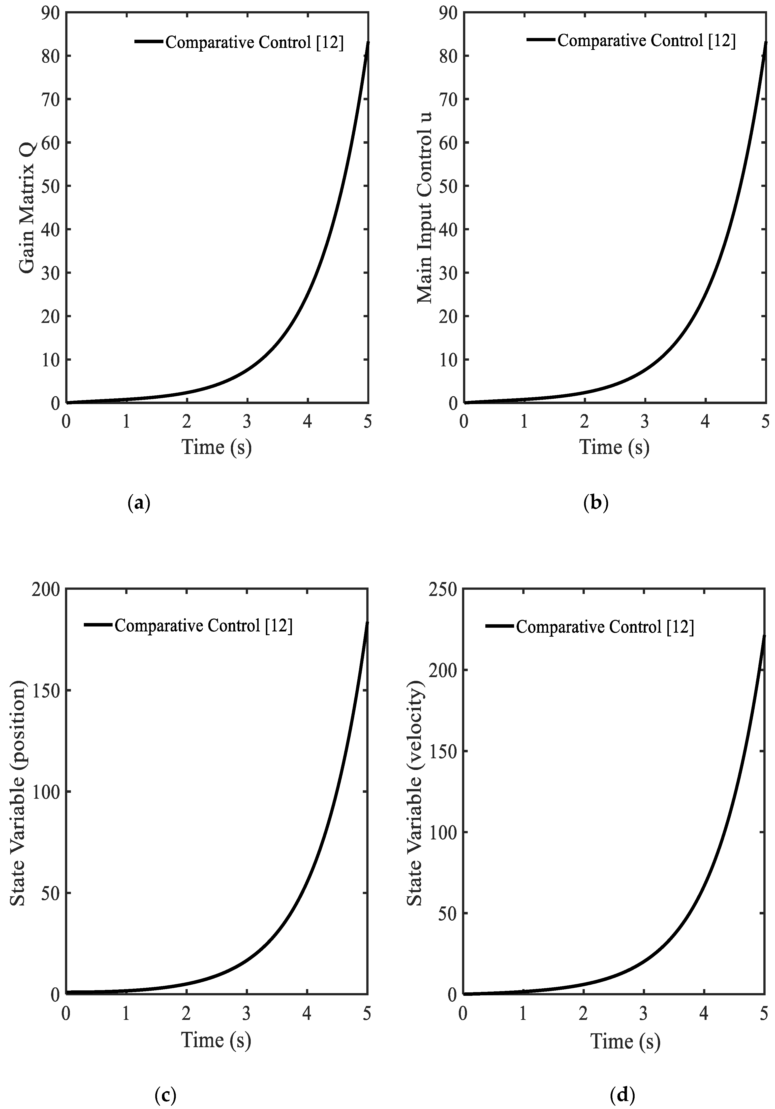
3.1. Example 1—Comparative Controller

In this simulation, the original linear model used in [12] is adopted as a comparative model as follows:
x ˙ e ( t ) = x e ( t ) + u ( t ) , x e ( 0 ) = 1
The initial parameter for this simulation is t [ 0 , 5 ] , M L ξ ( t ) = 1 , N L ξ ( t ) = 1 , and the cost function or criterion function is described as follows:
J = 50 | x e ( T ) | + 1 2 0 T ( u 2 ( t ) + x e 2 ( t ) ) d t
The solution of the comparative controller is obtained as follows:
x ˙ e ( t ) = x e ( t ) + Q L ξ * ( t ) s i g n ( x e ( t ) )
Q ˙ Δ L = | x e ( t ) | Q Δ L ( t )
In this simulation, the Runge-Kutta (RK) method is applied to solve the differential equations. It is remarked that the RK method is frequently used in real time systems [16,17,18]. Simulation results are shown in Figure 1. In Figure 1a, the gain function Q Δ L ( t ) is always increased its value increases. This point indicates that the optimized gain value cannot be found. Hence, the main control u * ( t ) is also not optimized as shown in Figure 1b. Because of the values of Q Δ L ( t ) and u * ( t ) , the system responses as state variables (position x e ( t ) , velocity x ˙ e ( t ) ) are not stable as shown in Figure 1c,d. In short, the system becomes unstable after applying the optimal controller [12]. In Reference [12], the gain matrix function (24) was obtained from the general form as follows:
Q ˙ Δ L ( t ) = N L ξ ( t ) | x L ξ ( t ) | G L ξ T Q Δ L ( t )
In the comparative controller, this gain matrix function has the signum (sign) function, which is not sufficient for controlling the system. This reason arises from the properties of the signum function where the default boundary in upper and lower values as 1 and −1. In [12], the final gain matrix value has been pointed out before the progress of the control action. In the conventional optimal control law, the time of convergence of the control could be predicted. However, this property cannot apply to the gain value. Thus, the shooting method is normally used for predicting the gain value [12]. However, the shooting method cannot be used for practical systems because it takes long time to find the final solution.

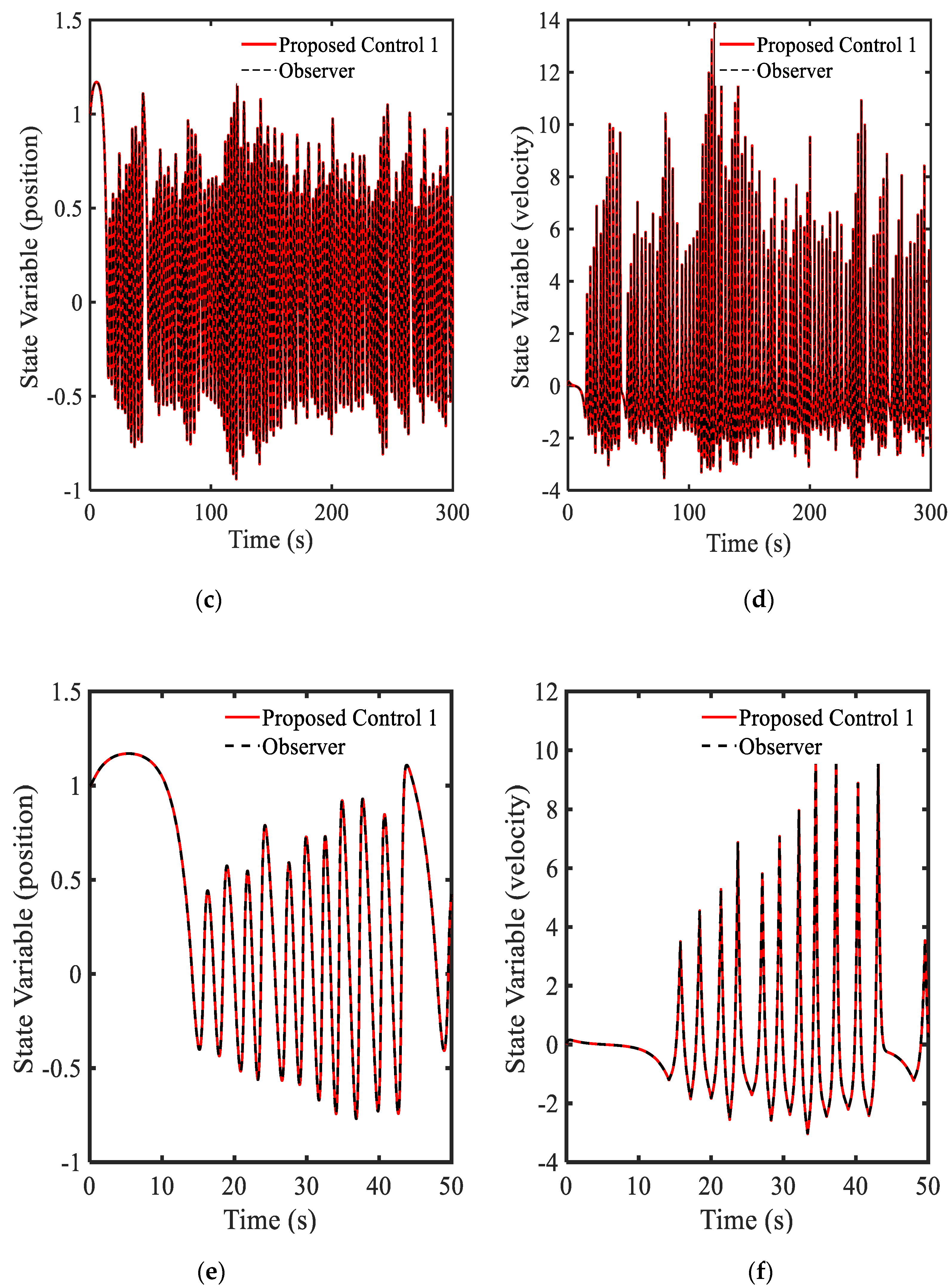
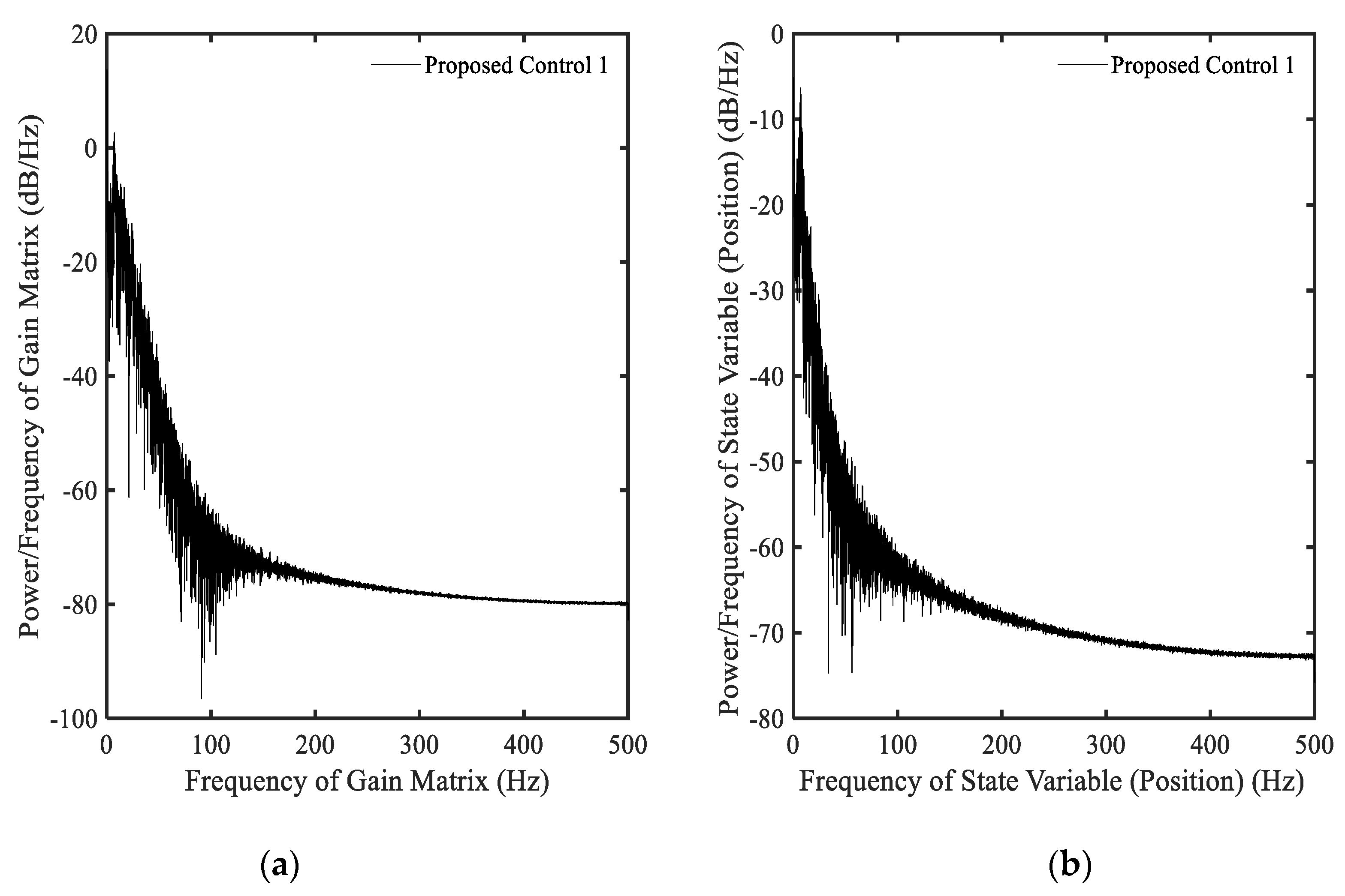
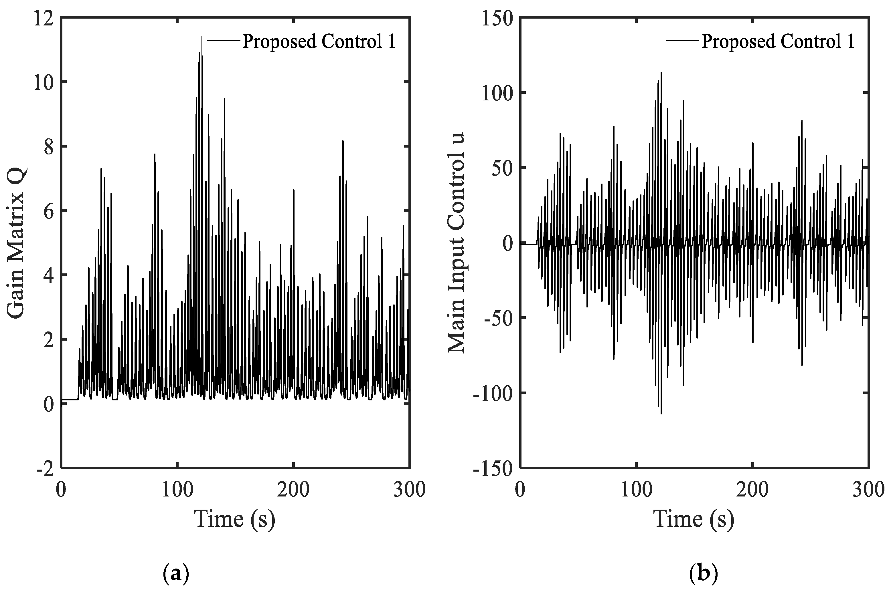
3.2. Example 2—Proposed Controller with Equation (12)

The model of Example 1 is used, but the gain matrix function shown in Equation (12) is utilized where the parameters are used as follows; t [ 0 , 300 ] , M L ξ ( t ) = 1.5 , N L ξ ( t ) = 1.2 , γ = 10 . The cost function is expressed as follows:
J 2 = 50 | x e ( T ) | γ + 1 2 0 T ( u 2 ( t ) + x e 2 ( t ) ) d t
The main input control is the given by:
u * ( t ) = γ Q L ξ * ( t ) s i g n ( x e ( t ) )
where Q L ξ * ( t ) is found from Equation (12) as follows:
Q ˙ Δ L ( t ) = | x e ( t ) | γ x e ( t ) Q Δ L ( t )
The proposed control in this simulation is named “the proposed control 1” for the convenience to distinguish from the other optimal controller used in other examples. In this simulation, the observer used in [19] is applied to evaluate the proposed control performances. Simulation results are shown in Figure 2a–f. The gain matrix Q Δ L ( t ) in Figure 2a is always changed depending upon its value, and the values are positive. This result has point out in Equation (20). Based on the variation of Q Δ L ( t ) , the main input control u * ( t ) is also changed with the values in positive and negative areas as shown in Figure 2b. The response of the system is shown in Figure 2c–f. Because the original system given by Equation (21) is to be vibrated due to the main input control u * ( t ) , the state variable are also vibrated as shown in Figure 2e,f. The results clearly show that the proposed control with gain matrix function given in Equation (12) can provide better performance than the compared control shown in Figure 1. In Figure 3, the response of the system following the power spectral density (PSD) is presented including the gain matrix Q Δ L ( t ) and the state variable x e ( t ) . The value of the gain matrix is stable with the increasing frequency as shown in Figure 3a. Hence, the position x e ( t ) is also stable as shown in Figure 3b. This performance directly indicates that the optimal controller with the new gain function given by Equation (12) can guarantee the stability of the system with better performances.

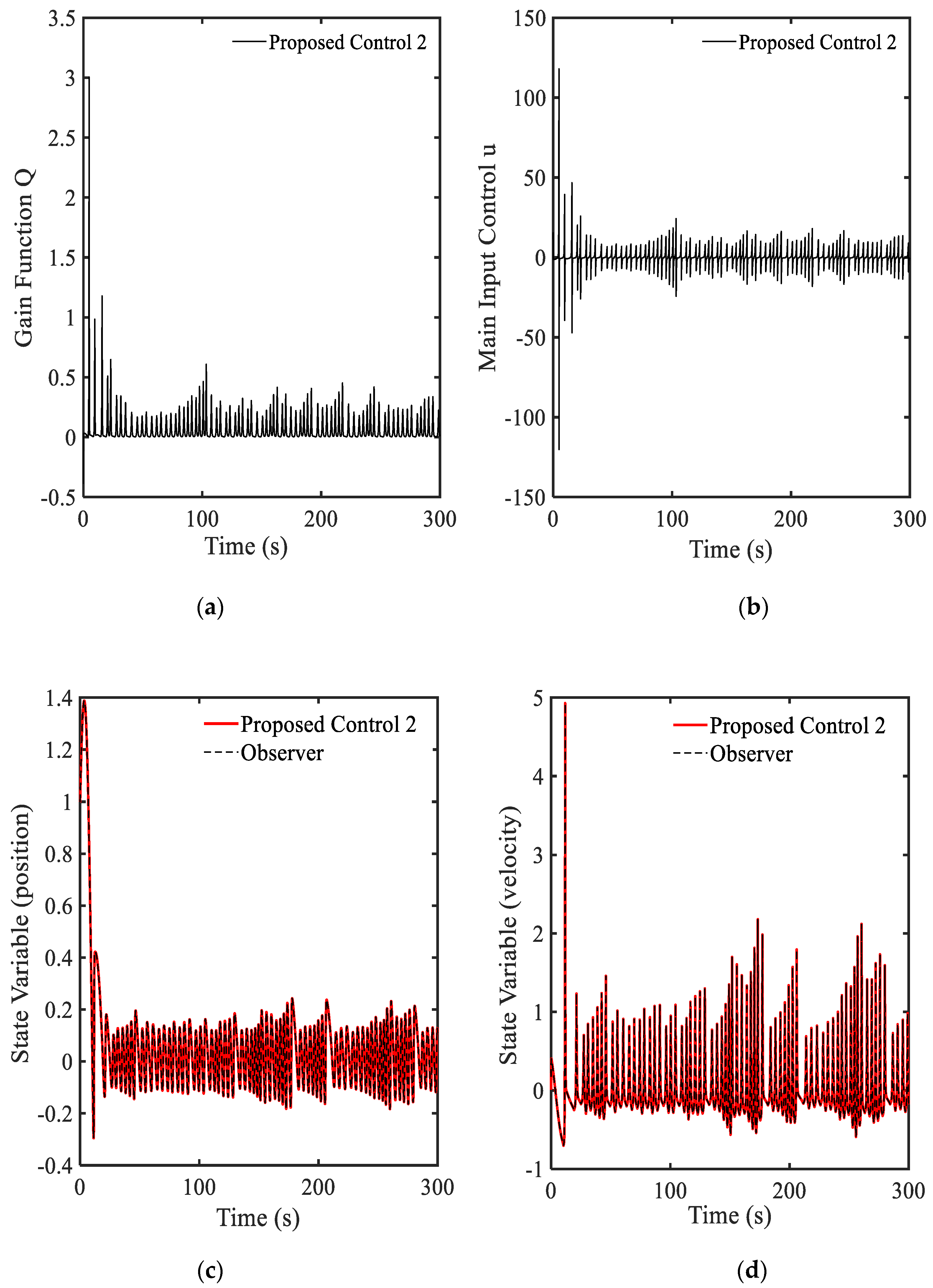
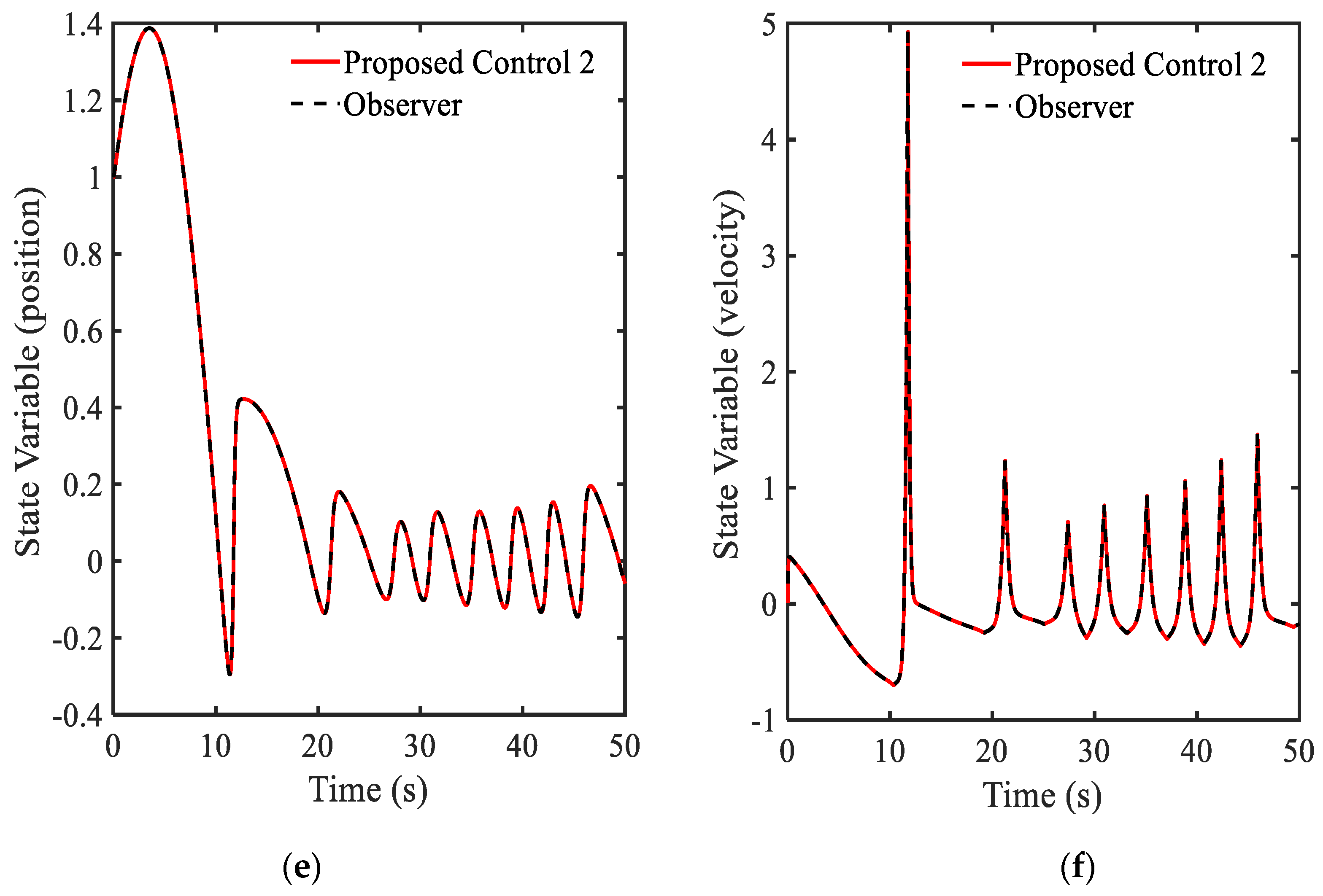
3.3. Example 3—Proposed Controller with Equation (7)

In this simulation, the same mode used in 3.2 is adopted with different gain matrix function (7) as follows:
Q ˙ Δ L ( t ) = N L ξ ( t ) x e 2 ( t ) γ x e ( t ) Q Δ L ( t )
The parameters of t [ 0 , 300 ] , M L ξ ( t ) = 1.5 , N L ξ ( t ) = 1.2 , and γ = 40 are used in this example. The proposed method is named “the proposed control 2”. In this simulation, the observer developed in [19] is also applied. Simulation results are shown in Figure 4 and Figure 5. It is clearly seen that after applying the proposed method 2, the magnitudes of all parameters are dramatically decreased as shown in Figure 4. In Figure 5, the PSDs of both proposed control 1 and proposed control 2 are depicted. The results prove that the proposed control 2 provides better control performance than the proposed control 1 in both of gain matrix and position of the system. In addition, the energy using for control action shown in Figure 5 indicates that the requirement of control energy of the proposed control 2 is less than that of the proposed control 1. Hence, by applying the proposed control 2, two benefits can be achieved in the sense of stability and energy saving.

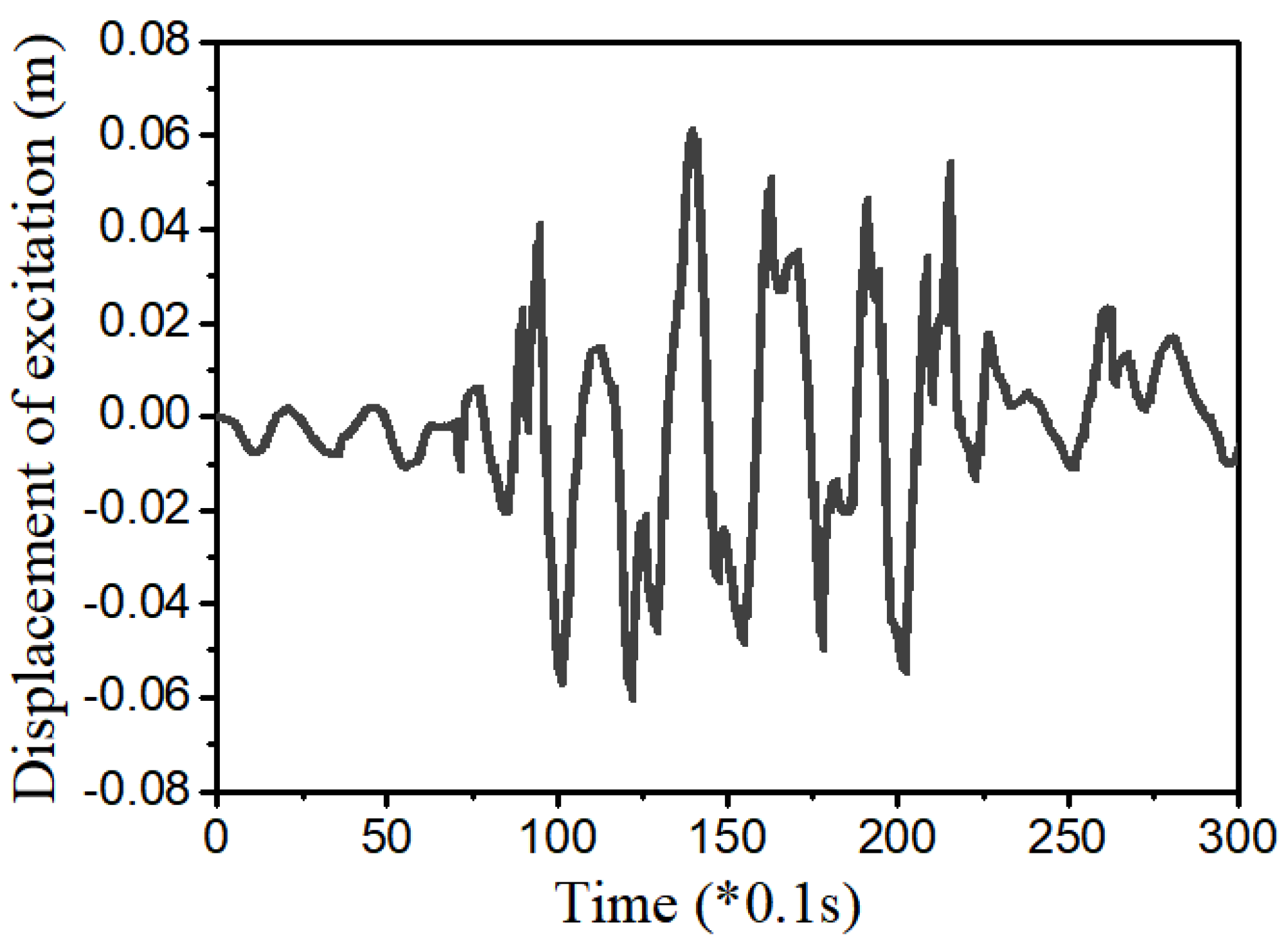
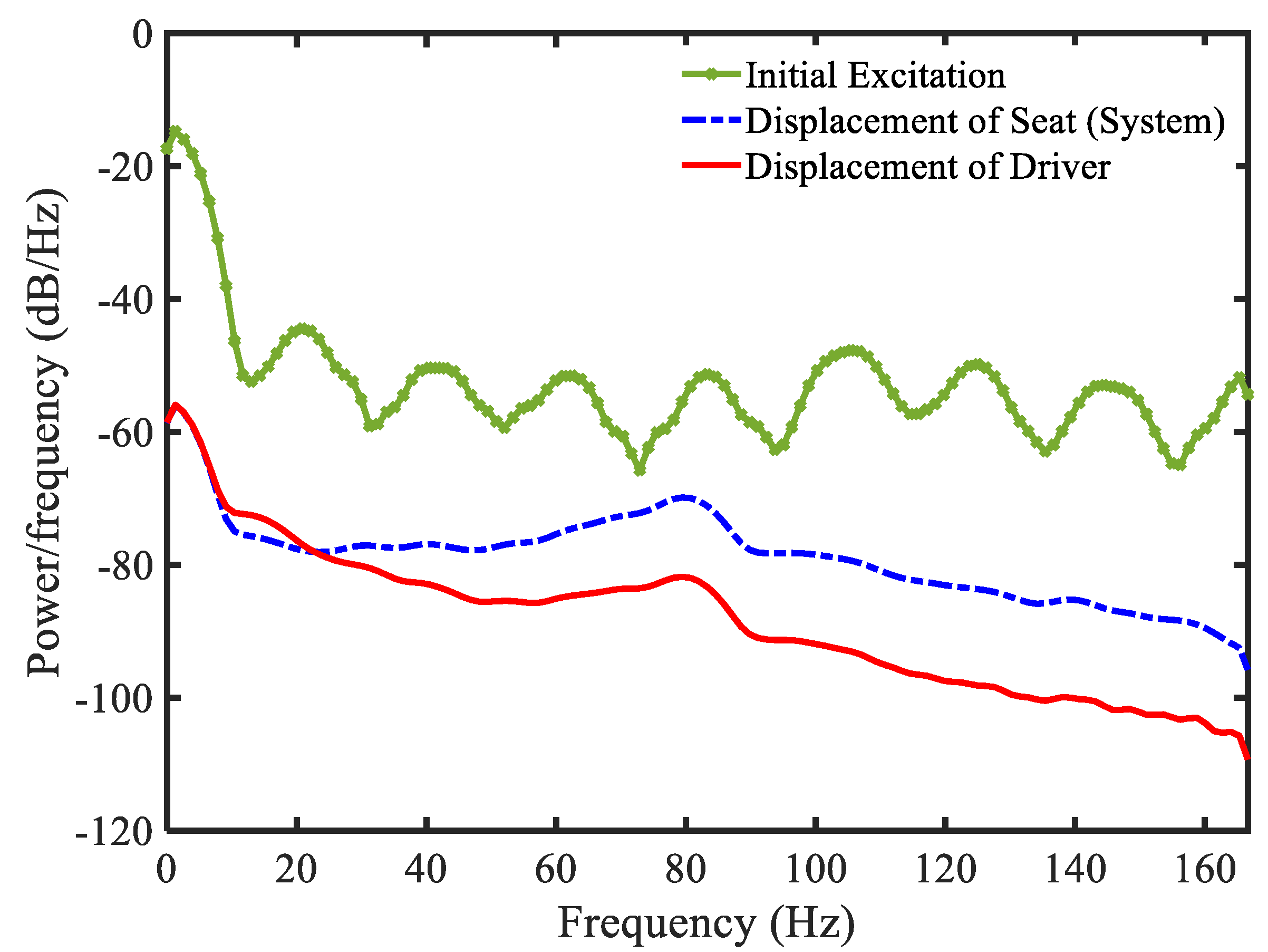
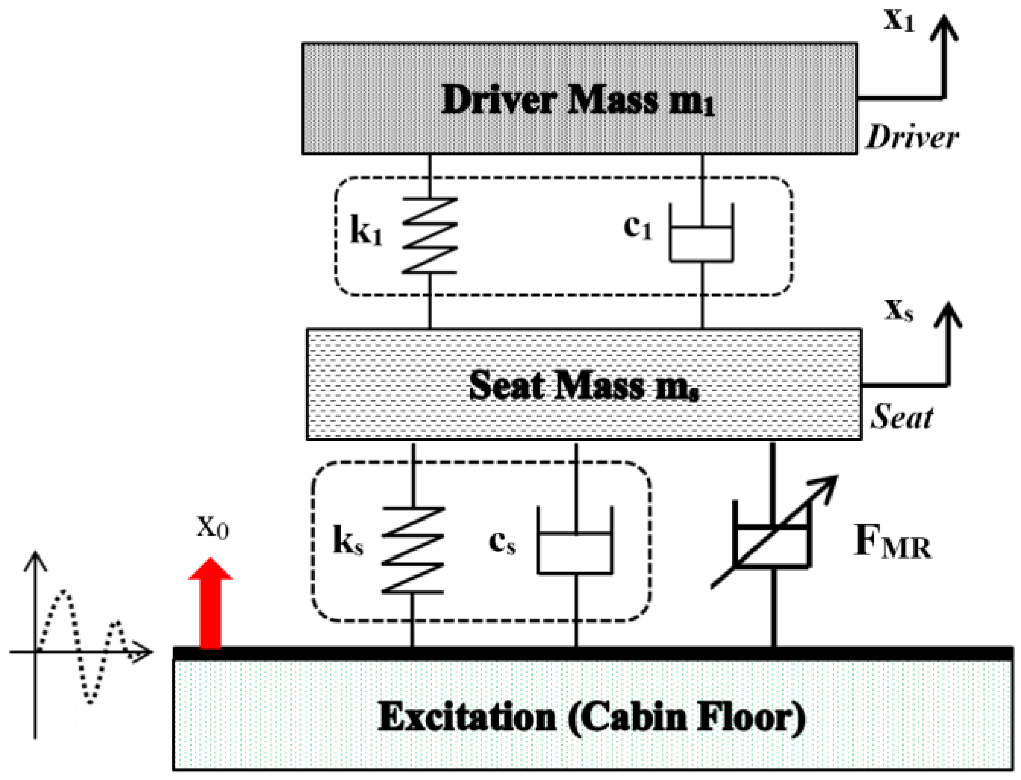
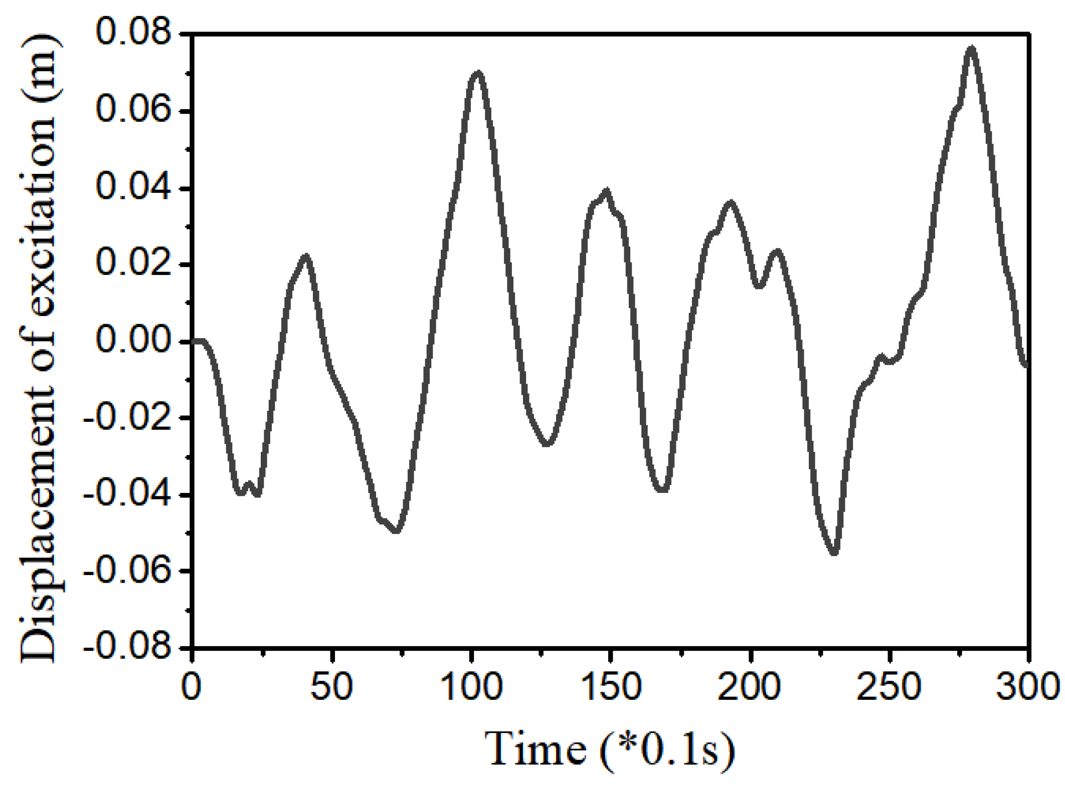
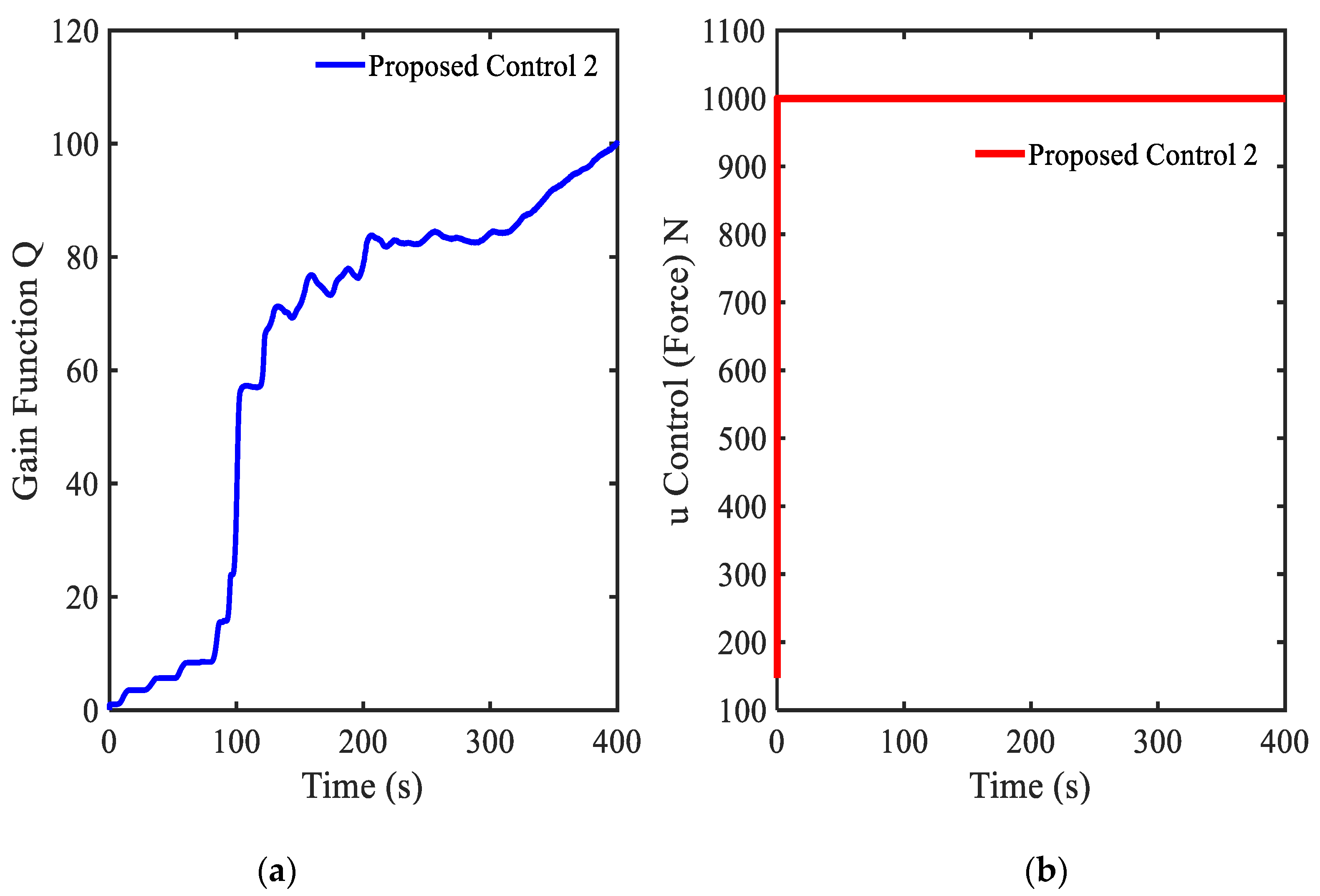
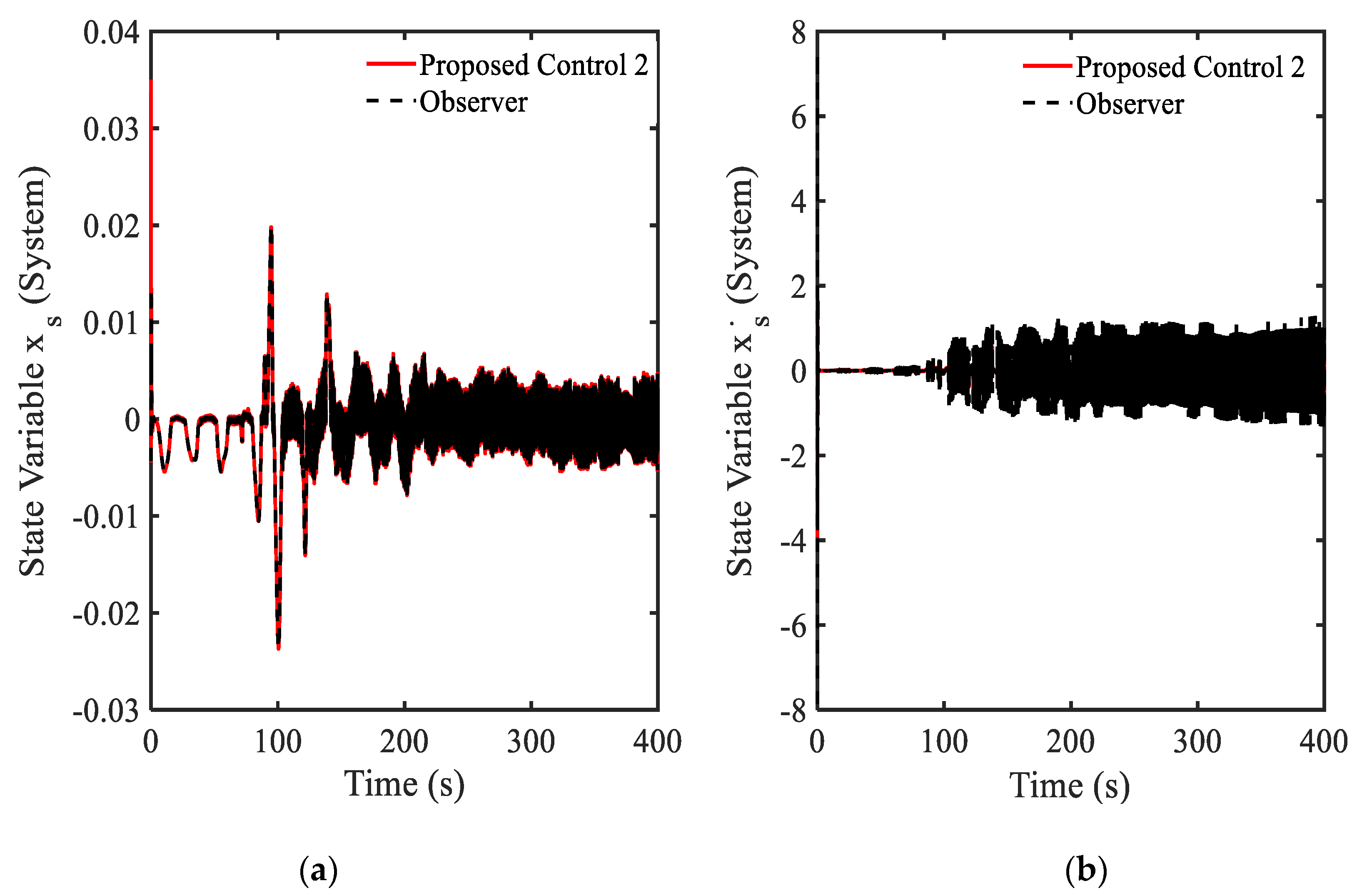
3.4. Example 4—Proposed Controller for Vibration Control with Random Bump Road Excitation (1)

In order to demonstrate effective applicability of the proposed optimal control law, a vehicle seat suspension system featuring MR (magnetorheological) damper previously studied by the authors [16,17,18] is adopted. The mechanical model of the seat suspension is shown in Figure 6, and from this model, the governing equations of the system are derived as follows:
m l s x ¨ s = k s ( x s x 0 ) c l s ( x ˙ s x ˙ 0 ) + k l 1 ( x 1 x s ) + c l 1 ( x ˙ 1 x ˙ s ) + F d M R
m l 1 x ¨ 1 = k l 1 ( x 1 x s ) + c l 1 ( x ˙ 1 x ˙ s )
In the above, xs and x1 represent the displacement of the sprung mass and driver mass, respectively. The variables ki and ci denotes the corresponding coefficients of the spring and damper. Moreover, x0 is the excitation displacement and FMR represents the magnetic field-dependent damping force of MR damper. The state-space model of the system is derived from the above equations as follows:
x ˙ l 11 = x ˙ s = x l 22 x ˙ l 22 = f l 11 ( x l 11 , x l 22 , x l 33 , x l 44 ) + g l 11 ( x l 11 , x l 22 , x l 33 , x l 44 ) u x ˙ l 33 = x ˙ 1 = x l 44 x ˙ l 44 = f l 22 ( x l 11 , x l 22 , x l 33 , x l 44 )
where:
f l 11 ( x l 11 , x l 22 , x l 33 , x l 44 ) = k l s m l s ( x l 11 x 0 ) c l s m l s ( x l 22 x ˙ 0 ) + k l 1 m l s ( x l 33 x l 11 ) + c l 1 m l s ( x l 44 x l 22 ) g l 11 ( x l 11 , x l 22 , x l 33 , x l 44 ) = 1 m l s u = F d M R f l 22 ( x l 11 , x l 22 , x l 33 , x l 44 ) = k l 1 m l 1 ( x l 33 x l 11 ) c l 1 m l 1 ( x l 44 x l 22 )
It is noted that x l 11 , x l 22 , x l 33 , x l 44 are variables related to x s and x 1 of the system. The calculated result of u = F d M R must be converted to the input signal to generate the required magnetic field for MR damper. The parameters of the seat suspension system used in this simulation are listed in [16,17,18]. The following parameters of t [ 0 , 300 ] , M L ξ ( t ) = 20 , N L ξ ( t ) = 20 , and γ = 100 are chosen for the simulation.
In this simulation, the random road profile shown in Figure 7 is used as an excitation signal from the ground. It is seen from Figure 8a that the gain value Q Δ L ( t ) is always changed and its final value is the positive number. The main control u * ( t ) shown in Figure 8b is also changed following the variation of the vibration. The results of the state system and states of the driver are shown in Figure 9, Figure 10 and Figure 11. In Figure 9a, it is shown that the vibration of the seat system is converged to boundary of (−0.005, 0.005) m. The vibration of the seat is decreased with large difference after using the proposed control 2. In addition, the velocity shown in Figure 9b is approximately zero. It is observed from Figure 10 that the state variables indicating vibration levels are effectively decreased. Subsequently, the state variables of the driver are also decreased as shown in Figure 11. The power spectral density diagram of the state variables is presented in Figure 12. These results prove that the proposed control 2 can provide high performance for vibration control of a complicated control system without degradation of the stability. It is noted here that in this simulation of the proposed control 2 has been used with the new gain function matrix given in Equation (7), which is proposed in this work.

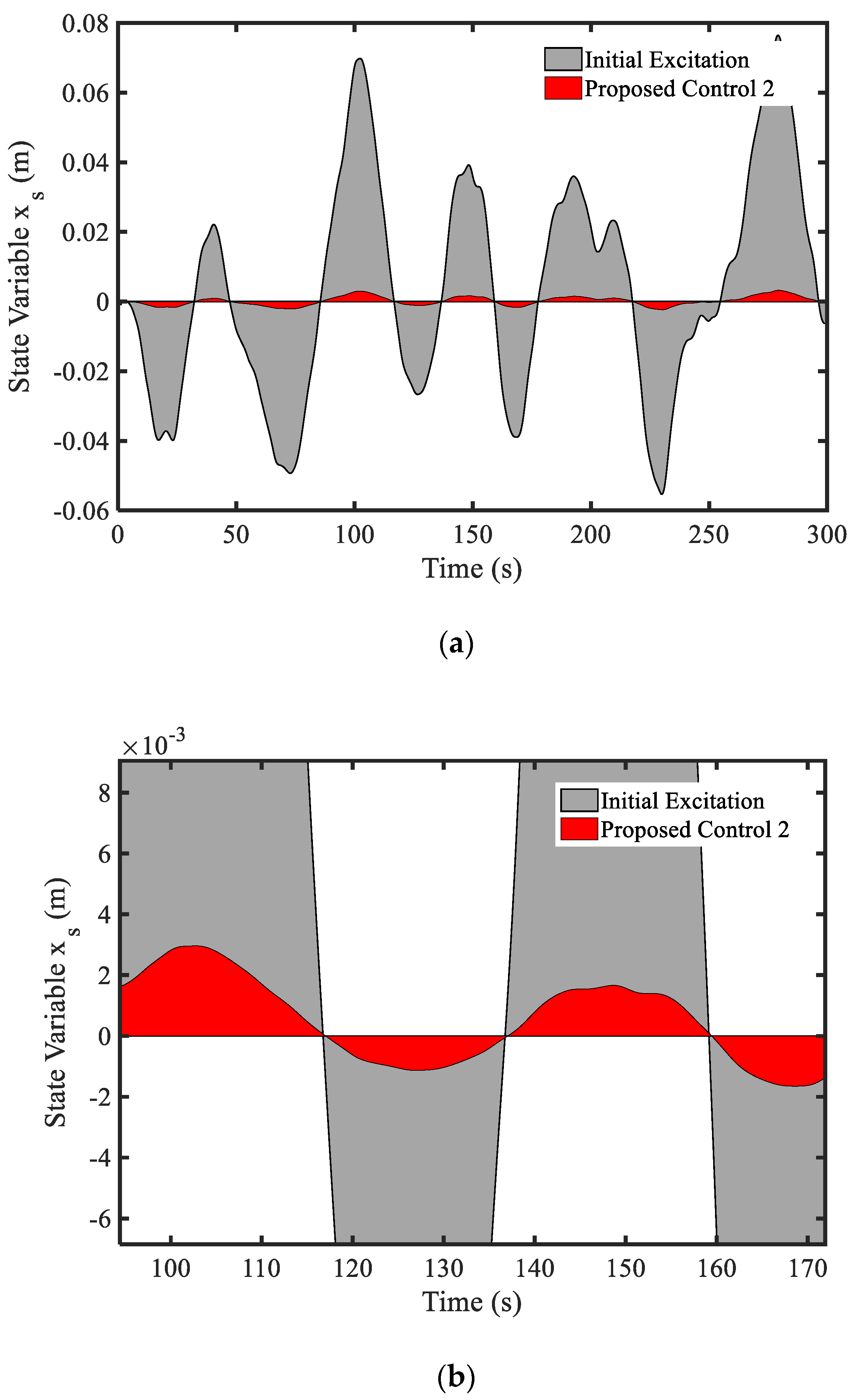
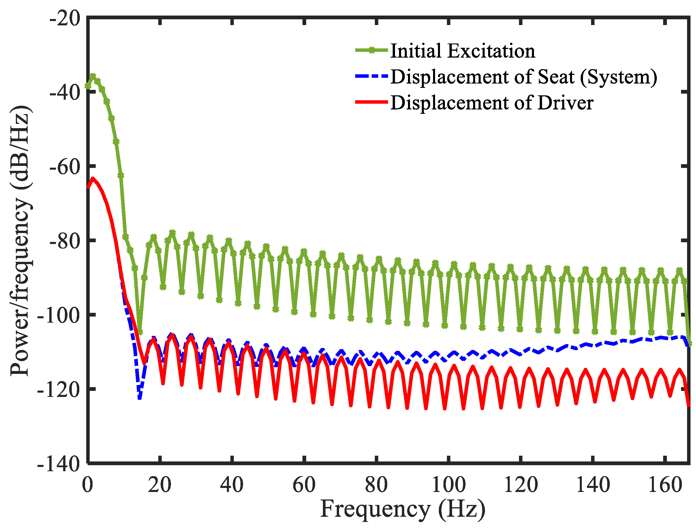
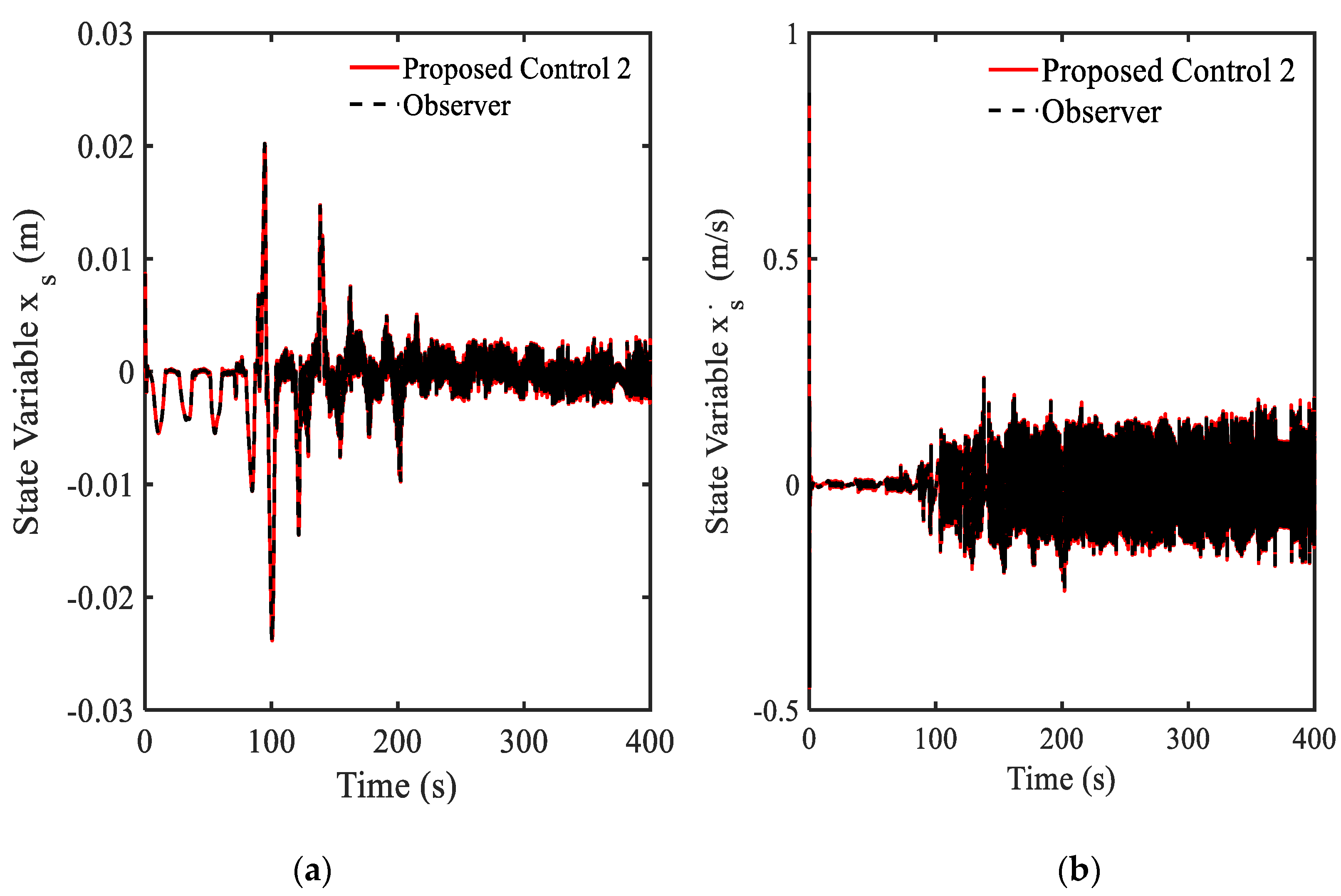
3.5. Example 5—Proposed Controller for Vibration Control with Random Step Wave Excitation (2)

As a final simulation, the effect of the gain parameters are investigated by adopting the following parameters of t [ 0 , 400 ] , M L ξ ( t ) = 160000 , N L ξ ( t ) = 60000 , and γ = 10 , those are different from those used in Example 4. Moreover, to reflect more practical applicability of the proposed control 2, the random step wave road excitation shown in Figure 13 is chosen in this simulation. Results of simulation are presented in Figure 14, Figure 15, Figure 16 and Figure 17. From Figure 14a, it is seen that the gain value Q Δ L ( t ) is the positive value. The main control u * ( t ) in Figure 14b obtains the maximum damping force of MR damper as 1000 N. This point shows that the disturbance (road excitation) is severe, and hence, needs more energy for effective vibration control. The state variables (displacement and velocity) at system and driver position are shown in Figure 15 and Figure 16. It is clearly observed from that unwanted vibrations are well controlled at both positions. The power spectral density (PSD) diagram of the state variables is shown in Figure 17. These results show that the initial vibration of the system and driver are decreased with large values after applying the controller. The results presented in this simulation also demonstrate that the proposed control 2 is very effective for vibration control of more realistic systems subjected to severe external disturbances. It is noted here that in this simulation of the proposed control 2 has been used with the new gain function matrix given in Equation (7), which is proposed in this work. From examples 4 and 5, it is known that the desired (or required) control performances can be achieved by changing the gain parameters associated with the gain function matrix.

4. Conclusions

In this study, a new optimal control law was formulated using the sliding mode controller, whose gains are adjustable and of which the control performances were evaluated by adopting several illustrative examples. In the formulation of the controller, the objective function of the Bolza-Meyer criterion was adopted to make the value of the gain larger than 1. This is a salient point to resolve some drawbacks conventional optimal controllers in which the values of the definite symmetry matrices are less than 1. By adopting the adjustable gain values, the non-negative definite symmetric matrix function of the Meyer term is reduced and hence the energy consumption for control action is also decreased. In order to verify the benefits of the proposed optimal control law with the new gain function matrix, five illustrative examples are adopted and control performances are evaluated based on three criteria: control gain index, main input control index, and the state index through the power spectral density (PSD) figures. After showing excellent control performance of the proposed controller in simple systems, it was applied to vibration control of the vehicle seat suspension system subjected to both the random bump road excitation and random step wave excitation. It was shown that unwanted vibration at the driver position is well controlled by implementing the proposed optimal controller showing the low power and high stability. The results prove that the proposed gain function and chosen matrices can satisfy for the systems as given Table 1. Therefore, the results presented in this work are self-explanatory justifying that the proposed optimal control will be applied to diverse linear time-varying systems subjected to disturbances. It was finally remarked that as a second phase of this work, an experimental implementation through a real time feedback control will be undertaken by adopting the seat suspension system treated in this work.

Author Contributions

Conceptualization: D.X.P and S.-B.C., formula analysis: V.M. and D.X.P. and data curation: V.M. and D.X.P, writing and editing: D.X.P. and S.-B.C., review and funding acquisition: S.-B.C.

Funding

This work was supported by the National Research Foundation of Korea (NRF) grant funded by the Korea government (MEST) (No. 2017R1A2B3003026). This financial support is gratefully acknowledged.

Conflicts of Interest

The authors declare no conflict of interest.

References

  1. Modares, H.; Lewis, F.L.; Naghibi-Sistani, M.B. Adaptive optimal control constrained input systems using policy iteration and neural networks. IEEE Trans. Neural Netw. Learn. Syst. 2013, 24, 1513–1525. [Google Scholar] [CrossRef] [PubMed]
  2. Luo, W.; Chu, Y.C.; Ling, K.V. Inverse optimal adaptive control for attitude tracking of spacecraft. IEEE Trans. Autom. Control 2005, 50, 1639–1654. [Google Scholar]
  3. Bian, T.; Jiang, Y.; Jiang, Z.P. Decentralized adaptive optimal control of large scale systems with application to power systems. IEEE Trans. Ind. Electron. 2015, 62, 2439–2447. [Google Scholar] [CrossRef]
  4. Fan, Q.Y.; Yang, G.H. Adaptive nearly optimal control for a class of continuous-time nonaffine nonlinear systems with inequality constraints. ISA Trans. 2017, 66, 122–133. [Google Scholar] [CrossRef] [PubMed]
  5. Kim, S.; Kwon, S. Nonlinear optimal control design for underactuated two-wheeled inverted pendulum mobile platform. IEEE/ASME Trans. Mechatron. 2017; 22, 2803–2808. [Google Scholar]
  6. Xia, Y.; Yin, M.; Zou, Y. Implications of the degree of controllability of controlled plants in the sense of LQR optimal control. Int. J. Syst. Sci. 2018, 49, 358–370. [Google Scholar] [CrossRef]
  7. Yin, H.; Chen, Y.H.; Yu, D. Rendering optimal design in controlling fuzzy dynamical systems: A cooperative game approach. IEEE Trans. Ind. Inform. 2019, 15, 4430–4441. [Google Scholar] [CrossRef]
  8. Jin, W.; Kulić, D.; Lin, J.F.S.; Mou, S.; Hirche, S. Inverse optimal control for multiphase cost functions. IEEE Trans. Robot. (Early Access) 2019. [Google Scholar] [CrossRef]
  9. Basin, M.; Calderon-Alvarez, D.; Ferrara, A. Sliding mode regulator as solution to optimal control problem. In Proceedings of the 47th IEEE Conference on Decision and Control, Cancun, Mexico, 9–11 December 2008; pp. 2184–2189. [Google Scholar]
  10. Basin, M.; Calderon-Alvarez, D. Optimal controller for uncertain stochastic polynomial systems. J. Frankl. Inst. 2009, 346, 206–222. [Google Scholar] [CrossRef]
  11. Basin, M.V.; Rodríguez-Ramírez, P.C. Sliding mode regulator as solution to optimal control problem for non-linear polynomial systems. J. Frankl. Inst. 2010, 347, 910–922. [Google Scholar] [CrossRef]
  12. Basin, M.; Rodriguez-Ramirez, P.; Ferrara, A.; Calderon-Alvarez, D. Sliding mode optimal control for linear systems. J. Frankl. Inst. 2012, 349, 1350–1363. [Google Scholar] [CrossRef]
  13. Li, Y.M.; Min, X.; Tong, S. Adaptive fuzzy inverse optimal control for uncertain strict-feedback nonlinear systems. IEEE Trans. Fuzzy Syst. (Early Access) 2019. [Google Scholar] [CrossRef]
  14. Zeng, T.; Ren, X.; Zhang, Y.; Li, G.; Na, J. An Integrated optimal design for guaranteed cost control of motor driving system with uncertainty. IEEE/ASME Trans. Mech. (Early Access) 2019. [Google Scholar] [CrossRef]
  15. Zhang, Y.; Li, S.; Liu, X. Adaptive near-optimal control of uncertain systems with application to underactuated surface vessels. IEEE Trans. Control Syst. Technol. 2017, 26, 1204–1218. [Google Scholar] [CrossRef]
  16. Choi, S.B. Vibration control of a ship engine system using high-load magnetorheological mounts associated with a new indirect fuzzy sliding mode controller. Smart Mater. Struct. 2015, 24, 025009. [Google Scholar]
  17. Do Xuan Phu, D.K.S.; Choi, S.B. Design of a new adaptive fuzzy controller and its application to vibration control of a vehicle seat installed with an MR damper. Smart Mater. Struct. 2015, 24, 085012. [Google Scholar]
  18. Huy, T.D.; Mien, V.; Choi, S.B. A new composite adaptive controller featuring the neural network and prescribed sliding surface with application to vibration control. Mech. Syst. Signal Process. 2018, 107, 409–428. [Google Scholar]
  19. Ciccarella, G.; Dalla Mora, M.; Germani, A. A Luenberger-like observer for nonlinear systems. Int. J. Control 1993, 57, 537–556. [Google Scholar] [CrossRef]
Figure 1. Simulation results of the comparative optimal controller in [12]: (a) gain function Q Δ L ( t ) , (b) main control u * ( t ) , (c) state variable (position) x e ( t ) , (d) state variable (velocity) x ˙ e ( t ) .
Applsci 09 05050 g001
Figure 2. Simulation results of the proposed control 1 with Equation (12): (a) gain function Q Δ L ( t ) , (b) main control u * ( t ) , (c) state variable x e ( t ) , (d) state variable x ˙ e ( t ) , (e) large view of state variable x e ( t ) , (f) large view of state variable x ˙ e ( t ) .
Applsci 09 05050 g002aApplsci 09 05050 g002b
Figure 3. Power Spectral Density (PSD) of the proposed control 1 with Equation (12): (a) gain function Q Δ L ( t ) , (b) state variable x e ( t ) .
Applsci 09 05050 g003
Figure 4. Simulation results of the proposed control 2 with Equation (7): (a) gain function Q Δ L ( t ) , (b) main control u * ( t ) , (c) state variable x e ( t ) , (d) state variable x ˙ e ( t ) , (e) large view of state variable x e ( t ) , (f) large view of state variable x ˙ e ( t ) .
Applsci 09 05050 g004aApplsci 09 05050 g004b
Figure 5. Power spectral density (PSD) of the proposed control 1 with Equation (12) and the proposed control 2 with Equation (7): (a) gain function Q Δ L ( t ) , (b) state variable x e ( t ) .
Applsci 09 05050 g005
Figure 6. Model of the seat suspension.
Applsci 09 05050 g006
Figure 7. Random bump road excitation.
Applsci 09 05050 g007
Figure 8. Control results under random bump road excitation: (a) gain function Q Δ L ( t ) , (b) main control u * ( t ) .
Applsci 09 05050 g008
Figure 9. Vibration control results at the seat position under random bump road excitation: (a) displacement, (b) velocity.
Applsci 09 05050 g009
Figure 10. State variable (displacement) at the seat position: (a) general view, (b) large view.
Applsci 09 05050 g010
Figure 11. Vibration control results at the driver position under random bump road excitation: (a) displacement, (b) velocity.
Applsci 09 05050 g011
Figure 12. Power spectral density of the proposed control system under random bump road excitation.
Applsci 09 05050 g012
Figure 13. Random step wave road excitation.
Applsci 09 05050 g013
Figure 14. Control results under random step wave road excitation: (a) gain function Q Δ L ( t ) , (b) main control u * ( t ) .
Applsci 09 05050 g014
Figure 15. Vibration control results at the seat position under random step wave road excitation: (a) displacement, (b) velocity.
Applsci 09 05050 g015
Figure 16. Vibration control results at the driver position under random step wave road excitation: (a) displacement, (b) velocity.
Applsci 09 05050 g016
Figure 17. Power spectral density of the proposed control system under random step wave road excitation.
Applsci 09 05050 g017
Table 1. Summarization of gain matrix function and chosen matrices of examples.
Gain Matrix FunctionChosen Matrices
PropertyValuePropertyValue
Example 2PositiveNot fixed and change following the systemNot fixed with unit matrix M L ξ ( t ) = 1.5 , N L ξ ( t ) = 1.2
Example 3PositiveNot fixed and change following the systemNot fixed with unit matrix M L ξ ( t ) = 1.5 , N L ξ ( t ) = 1.2
Example 4PositiveNot fixed and change following the systemNot fixed with unit matrix M L ξ ( t ) = 20 , N L ξ ( t ) = 20
Example 5PositiveNot fixed and change following the systemNot fixed with unit matrix M L ξ ( t ) = 160000 , N L ξ ( t ) = 60000

