Abstract
A cold chain for perishable fresh products aims to preserve the quality of the products under the control of a predefined temperature range. To satisfy the delivery conditions within appropriate time windows, the most critical operations in cold chain management is the transportation and distribution of fresh products. Due to rapid population growth and increasing demand for high-quality fresh foods, it becomes critical to develop advanced transportation and distribution networks for fresh products, particularly in urban areas. This research aims to design different scenarios based on mathematical models for fresh products transportation and distribution network in the Bangkok metropolitan area using Geographic Information system (GIS). The proposed methodology integrates location–allocation and vehicle routing problem analysis. The performance of all possible scenarios is evaluated and compared by considering the number of required distribution centers and trucks, total travel time, total travel distance, as well as fairness among drivers. The results of the scenario analysis highlight that the alternative scenarios show a better performance as compared to the current network. In addition, the administrator can make a different decision among several alternatives by considering different aspects, such as investment cost, operating cost, and balance of using available resources. Therefore, it may help a public officer to design the fresh products logistics network considering actual demand and traffic conditions in Bangkok.
1. Introduction
The cold chain for the perishable products is defined as the entirety of supply chain operations and processes to ensure the temperature control within the predefined range [1]. The core function of the cold chain is to monitor the temperature in order to preserve the integrity and the quality of products and to guarantee the shelf life of goods [1]. However, transportation of perishable products and associated logistics operations pose many challenges for the cold chain [2].
Specifically, there exists the general requirement for keeping the products as safe as possible during transportation. In addition, products should be delivered within the predefined time window and, at the same time, meet the expected food quality. These factors complicate the design and planning of the fresh products distribution network [3]. In addition, owing to the increased consumer awareness and government regulations on food safety, several issues have continuously been addressed as the most important problems in the foodservice industry [4].
To cope with the rapidly growing population and the ever-increasing demand for high-quality fresh food, a more advanced transportation system for fresh food delivery is needed, particularly in urban areas [5]. In this context, Bangkok metropolitan, the urban agglomeration of Bangkok, is a most representative case where an advanced fresh food transportation network is urgently needed. Bangkok metropolitan includes Bangkok city and five surrounding provinces: Pathum Thani province (north of Bangkok), Nonthaburi province (northwest of Bangkok), Nakhon Pathom province (west of Bangkok), Samut Sakhon (southwest of Bangkok), and Samut Prakan (south of Bangkok). These areas around the Bangkok metropolitan have become some of the fastest growing metropolises in the world. The estimated population is 16.2 million as of 2019 [6].
Bangkok is the center of commerce and trade in Thailand and is also relied heavily upon by companies across the Indochina Peninsula; however, because of the high number of private vehicles and the insufficient supply of transportation services, the traffic congestion is a major problem. It was categorized as the most populous and traffic-congested city in the country by a landslide. This problem has huge impacts on businesses in the logistics and distribution. A high number of private vehicles and the insufficient supply of transportation services lead to congestion problems in Bangkok city [7]. In the global index compiled by TomTom traffic index, Bangkok has been ranked the second lowest in the world. During the morning rush hour, extra travel time increases by about 91%, while, during the evening rush hour, the increase in travel time amounts to 118% [8]. According to a recent survey of Ministry of Transport, the average speed of vehicles in the morning rush hour was 15 km per hour (km/h) [9]; however, the lowest average in the Southern Bangkok was recorded 10.1 km/h. The worst congestion road is mainly on Krung Thon Buri road in between Krung Thon Buri and Surasak intersection (5.1 km/h) [9].
Currently, Talaad Thai wholesale market is a major existing distribution center (DC) of fresh food in the central region of Thailand. It is also the biggest wholesale market in Southeast Asia. In addition, domestic consumption for fresh fruits and vegetables in Bangkok is mainly supported by Talaad Thai market. [5]. With an increase of urban freight movements, a single DC cannot efficiently handle the growing demand from customers while considering the distance, lead time, and internal operations in the warehouse, particularly when it comes to Just-In-Time (JIT) delivery of fresh products [10]. Therefore, a new transportation network design is necessary for fresh food distribution using multiple distribution centers (DCs) in Bangkok [10,11].
According to the development of the fresh fruit and vegetables distribution, the design of the transportation network should take into account the location and distribution from a wholesaler to DCs, and then deliver products from DCs to retailers. Therefore, the location-routing problem (LRP) model, which integrates the location–allocation problem (LAP) and vehicle routing problem (VRP), is used to design the network transportation for fresh fruits and vegetables in Bangkok.
The main contribution of this research can be categorized five-fold. First, we analyzed the current distribution network for fresh fruit and vegetables from the existing DC to retailers. We provided managerial insights for helping decision makers in charge of designing the distribution network to solve the major problems of the existing network. Second, we have suggested a framework of the two-phase sequential approach that consists of very well-known research problems, LAP, and vehicle routing problems with time window (VRPTW), using Geographic Information systems (GIS). Third, we have devised a systematic approach for designing transportation networks in the public sector by applying the closest facility, minimizing the number of locations, and maximizing coverage based on the exact location and the practical road conditions for urban transportation. Fourth, we compared the performance of eight different scenarios based on total travel time, total distance, number of required trucks, number of DCs, and fairness among drivers. The result of comparing analysis may help decision makers to design a new distribution network in order to support the increasing demand of fresh fruit and vegetables. Finally, the proposed network can improve the efficiency by reducing the travel distance and enhancing the fairness among drivers while satisfying several constraints.
The remainder of this research is organized as follows. Section 2 provides a review of relevant literature. Then, in Section 3, the proposed research background is introduced. In Section 4, we describe the research methodology used in this research. Scenario analysis and sensitivity analysis are presented and discussed in Section 5. Finally, conclusions, limitations, and directions of future research are discussed in Section 6.
2. Literature Review
The LRP is one of the major problems in designing a logistics network, with important implications for the entire supply chain [12]. There are several distinctive characteristics of the fresh products transportation that should be accounted for in solving the LRP. These characteristics include shelf life constraints and perishability of products, long production throughput time, seasonality in production, conditioned transportation and storage, product safety issues, and natural conditions that affect the quantity and quality of farm products [4,13].
Generally, the fresh chain logistics builds customer value by merging logistics activities related to perishable products with common business processes [14,15]. In one relevant study, Hsiao, Chen, and Chin [3] modeled and resolved a cold chain distribution planning problem for perishable foods by generating a distribution plan that ensured the fulfillment of customer requirements for various foods and food quality levels at the lowest cost.
Furthermore, Gallo, Riccardo, Giulia, and Riccardo [16] designed the sustainable cold chain for food distribution on the silk road belt. A mixed integer linear programming model was applied to minimize the total energy consumption deal with the cold chain operation. The case study focused on the distribution for the perishable product along the new Silk Road, Europe, and China. The results suggested an efficient route and transportation modes on the sustainability of the cold chain.
Similarly, Bosona, Nordmark, Gebresenbet, and Ljungberg [17] evaluated the performance of an integrated food distribution network (IFDN) in Sweden. LRP analysis was applied to analyze the data of 11 producers, 149 customers, and one DC. GIS tools and LAP techniques were used. Four scenarios of food distribution were identified and analyzed. The number of routes, visits, transport distance, and total time were compared.
Bozkaya, Yanik, and Balcisoy [18] integrated the LRP model and a hybrid heuristic solution methodology to solve the competitive multi-facility location problem. A GIS-based framework was used to store, analyze, and visualize all data, as well as to propose model solutions in the geographic project. Furthermore, Bosona, Nordmark, Gebresenbet, and Ljungberg [19] considered four different scenarios to investigate the existing flow of locally produced foods from producers to consumers in Sweden. In addition, a coordinated and efficient food distribution system for local food producers was developed. GIS and Route Logix software (version, Manufacturer, City, US State abbrev. if applicable, Country) were used to get more insight into the impact of the integration of local food systems.
In another relevant study, Hsiao, Chen, Lu, and Chin [20] investigated the problem of last-mile delivery of fresh fruits and vegetables through considering multiple practical scenarios. A last-mile routing with the quality concern for cold-chain delivery was considered. The results indicated that the fulfillment of various requirements of different customers and appropriate quality levels could be ensured using cost considerations.
In addition, Hsu and Liu [21] proposed a model of facilities planning for a multi-temperature joint distribution system. The problem of optimal application of multi-temperature logistics techniques for terminal and vehicle routing operations was solved by minimizing the total delivery cost. This study focused on the choice of appropriate short-and medium-term operational strategies. In addition, the authors analyzed the advantages and disadvantages of various logistic techniques to provide operators with a valuable reference.
Furthermore, Mejjaouli and Babiceanu [2] proposed two types of decisions models: stopping transportation and/or rerouting the shipments to a closer location. The decision-making related to every shipment or series of shipments was made in the cloud using temporary virtual machines (VMs). The VMs make operational decisions based on the evaluation of actual transportation conditions and location of shipped products against requirements and initial route and terminal market geographical location. The results of the optimization models using logistics data (full truckload, shipping points, end markets, distance, $/mile for transportation, harvest periods, weekly demand) showed significant savings. The proposed system could be used for multiple product types and multiple locations.
In another study, Hsu and Chen [5] proposed a model to analyze the operation strategy of a joint distribution system by considering the costs of carriers, transportation demand, and acceptable shipping charges with a time-dependent demand pattern. The results of this study suggest that carriers determine departure times of multi-temperature food with demand–supply interaction and prioritize food of medium temperature ranges, as delivering such foods generates more profit.
Serra and Marianov [22] investigated location problems in the public sector. Most public facility located models were found to use a p-median problem approaches and/or a covering problem (Location Set Covering Problems, LSCP, or Maximal Covering Location Problems(MCLP) to set the foundations of the formulation. The results showed that p-median and covering problems could be considered as benchmarks in the development of location models.
Furthermore, Wang, Tao, and Shi [23] proposed the minimum total costs in cold chain logistics by using an LRP model. A hybrid genetic algorithm with heuristic rules is designed to solve the model under the constraints of both benefit and environment. The carbon tax policies are suggested to analyze the impact of carbon tax on the total costs and carbon emission.
Similarly, Fazayeli, Eydi, and Kamalabadi [24] integrated the multimodal routing and location-routing problems for considering in worldwide businesses. The problem consists with two dimensions: a multimodal network is to move products from producer to depots and a location routing network is to deliver products from depots to customers. A mixed-integer mathematical fuzzy model was presented for the proposed problem. The results suggested that time windows and fuzzy demands increased overall cost and time and imposed more difficulty on the problem. Moreover, comparing algorithm values and solution time indicated performance of the proposed algorithm.
Ma, Wu, and Dai [25] proposed the combined order selection and time-dependent VRPTW in delivering perishable products. This study aimed to determine delivery order, service sequence, and timing to start a delivery task in order to maximize profit maximization.
Solak, Scherrer, and Ghoniem [26] introduced a new variant of location-routing problem, which is the stop-and-drop problem (SDRP) for nonprofit food distribution networks in day-to-day-operations. Trucks delivered food to multiple sites by considering service area and partner agencies travel. The integrated mixed-integer model applied to solve a set of delivery sites, and determine agencies sites and route scheduling. Moreover, the Bender implementation and logic-based Benders decomposition heuristics were also proposed in this paper to fix time limitations.
Musolino, Polimeni, and Vitetta [27] proposed a procedure for the solution of the VRP based on Network Fundamental Diagram (NFD). The proposed link travel time function to calculate reliable travel times are used for the solution of VRP to obtain optimal routes of freight vehicles. The results indicated that that the optimal routes contribute to avoid heavily congested links and portions of the network in urban areas.
Finally, Musolino, Rindone, Polimeni, and Vitetta [28] integrated location and vehicle routing problems for planning an Urban Distribution Center (UDC) based on the restocking demand scenarios in order to follow sustainability goals. This study aimed to support city logistics planning, evaluating cost and benefits of the logistics operators in Southern Italy. In addition, the proposed methodology can be applied to attain a trade-off among sustainability dimension regarding public and private needs.
In summary, from the literature review presented in Table 1, it can be concluded that several previous studies have investigated several solutions to solve the network design problem in fresh food logistics. In these previous studies, the LAP and VRP are the most widely applied approaches. Most of them focused on cost minimization as the economic dimension of sustainability, especially in private sector. However, only a few previous research works considered the social and environment dimensions. Moreover, a few previous studies on LRP considered the exact locations and real transporting routes among origins and destinations. Most previous studies presented the results of the optimal solutions were compared to the number of locations, travel distance, travel time, and the number of routes. Therefore, it is not easy to find research that focused on the public sector and considered fairness among drivers. Likewise, not many studies compared different approaches that aimed at minimizing facilities and maximizing coverage approach applied in the fresh fruit and vegetables transportation. It is possible to find that most of the previous research has considered LAP, VRP, VRPTW, or other related models, respectively. In this research, we have suggested the research framework by integrating the LAP and VRPTW. In addition, in this research, we have compared the different scenarios that consisted of various approaches such as the closest facility, minimum number of facilities, and maximizing coverage. The performance of all scenarios was evaluated by applying VRPTW considering the limited capacity of trucks from the limited number of DCs to all delivery points. By comparing with the quantitative metrics such as the number of required DCs and trucks, the travelling time and distance, and fairness among drivers, it may be possible to suggest a better alternative for an urban transportation network for distributing fresh fruits and vegetables.

Table 1.
Summary of literature review: location–allocation problem(LAP); vehicle routing problem (VRP); location-routing problem (LRP); vehicle routing problems with time window (VRPTW).
3. Research Background
Location and routing problems were some of the main concerns in logistics. To solve the problem of distribution for fresh fruits and vegetables, the framework which integrates LAP and VRPTW approaches is devised in this research. The presented framework can be divided into the following two-phase sequential approach. The first phase is to identify the location of fresh food distribution and demand allocation. The second phase is to design the routes for delivery and the number of vehicles required while minimizing the total travel distance while delivering fresh fruits and vegetable from wholesalers to retailers through DCs. The LAP and VRPTW are described as follows:
3.1. Location–Allocation
Location-allocation is divided into two sections: locating facilities and allocating demand points to the facilities. The purpose of LAP is to minimize the overall distance between demand points and facilities, maximize the number of demand points covered within a certain distance of facilities, maximize an apportioned amount of demand, and maximize the amount of demand captured in an environment of friendly and competing facilities [29]. This research aimed to find the minimum number of DCs or to find the location of DCs while maximizing coverage based on the predetermined the number of DCs that will be explained in further details.
3.1.1. Minimum Facility Location Problems
The objective of minimum facility location problem is to find the minimum number of facilities while covering all demand. It can be stated that each and every demand point has at least one server located within some distance or time standard [22]. When the cost of building facilities is not considered, a demand point inside the impedance cutoff has been allocated to the nearest facility [30]. The formulation of the model is as follows:
Sets:
= set of demand nodes (indexed by );
= set of eligible facility sites (indexed by );
Parameters
= ;
= the distance from potential facility location to demand node ;
= the distance standard for coverage;
Decision Variable:
Binary variable equals 1 if a facility is located at node j, 0 otherwise:
subject to
Note that is the set of all those candidate sites for the potential location of facilities that are within distance of demand node i. When a facility is located in any of the candidate sites, demand node i is covered. The objective in Equation (1) minimizes the number of facilities required. Constraints in Equation (2) ensure that there is at least one opened facility within standard distance s from each demand node [22].
3.1.2. Maximizing Coverage
Maximizing coverage is used to locate facilities based on the number of facilities, which, in this case, is determined by the decision maker. Additionally, facilities are often required to arrive at all demand points within a specified response time [30]. This model, called MCLP, seeks the location of a fixed number of facilities that are most probably insufficient to cover all demand within the standards, so the demand covered by the service is maximized [22]. The fixed number of facilities is a proxy for a limited budget [22]. Its formulation is as follows (see Equation (4)):
Sets:
= set of demand nodes (indexed by );
= set of eligible facility sites (indexed by );
Parameters
= the number of facilities to be deployed;
= the demand quantities at demand node ;
= ;
= the distance from potential facility location to demand node ;
= the distance standard for coverage;
Decision Variables:
= binary variable equals 1 if node is covered, 0 otherwise;
binary variable equals 1 if a facility is located at node , 0 otherwise.
subject to
The objective in Equation (4) maximizes the weighted sum of covered demand nodes. Constraints in Equation (5) state that the demand at node i is covered whenever at least one facility is located within the time or distance standard S. Constraint in Equation (6) gives the total number of facilities that can be sited [22].
3.2. Vehicle Routing with a Time Window
The VRP is one of the most significant problems in distribution management [17]. The VRP aims to provide a high level of customer service while complying with time windows [31]. The constraints are to complete the routes with available resources and within the time limits imposed by driver work shifts, driving speeds, and customer commitments [31].
In this research, we used the VRPTW, which is a generalization of the VRP where the service at any customer starts within a given time interval, called a time window [32]. The formulation of the model is as follows:
Sets:
= set of demand nodes (indexed by );
= set of eligible facility sites (indexed by );
= set of vehicles (indexed by );
= set of customers;
Parameters
= travel cost from node to node ;
= travel time from node to node ;
= demand of customer at node ;
= capacity of vehicle;
= earliest service time at node ;
= latest service time at node ;
Decision Variables:
= binary variable equals 1 if a fleet vehicle travels from node to node , 0 otherwise;
= arrival time of vehicle at node ;
= arrival time of vehicle at node ;
subject to
The objective function in Equation (8) minimizes not only the number of vehicles required, but also the total travel time, and total travel distance incurred by the fleet of vehicles. The constraints in Equation (9) certify that each customer is visited once, and Equation (10) indicates that a vehicle can be loaded up to its capacity. Equations (11)–(13) state that each vehicle is initially located at a distribution center, which we denote by 0; after arriving at a delivery point, it has to leave to another destination; finally, all vehicles must arrive at depot n + 1. The inequalities in Equation (14) establish the relationship between the vehicle departure time from a customer and its immediate successor. Finally, constraints in Equation (15) insist that time windows should be observed, and Equation (16) shows integrality constraints. Note that an unused vehicle is modeled by driving the empty route (0, n + 1) [32].
4. Methodology
The proposed methodology integrates location–allocation and vehicle routing problem analysis. Figure 1 shows the four-step of this research. Each step will be explained in further detail.
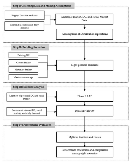
Figure 1.
Main steps of the proposed methodology.
4.1. Step I: Collecting Data and Making Assumptions
We assumed that the fresh products consist of producers, wholesalers, which are the central markets of each province, fresh products DC, retailers, and end customers. Most of the problems and issues of a distribution network for the fresh products arise from wholesalers to retailers. Therefore, in this research, we focused on two parts: from DC to retailer and from wholesaler to DC (see Figure 2). In the first part, each retailer was assigned to DC based on the distance. In the second part, the distribution from the wholesale market to the potential candidate DCs had to be analyzed based on travel distance, total demand of DCs, and production capacity of the wholesaler.
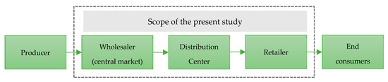
Figure 2.
Fresh products logistics.
4.1.1. Wholesale Market, DC, and Retail Market
The information and data collection for scenario analysis were performed based on the following set of assumptions:
- Location of existing DC: Talaad Thai market is the biggest wholesale market in Thailand and Southeast Asia for trading of agriculture goods. This existing DC supplies fresh fruits and vegetables to all of the main retailers in Bangkok.
- Location of eight candidate distribution DCs (see Table 2 and Figure 3): one of the development agendas of Thailand’s logistics development plan (2017–2021) was formulated for developing a fresh products distribution system to reduce cost and waste as well as flagship projects [33]. Moreover, Thailand’s agricultural development plan from 2017 to 2021 aims to promote agricultural supply chain management from producer to end customer [34] by encouraging the establishment of service centers (facilities) in the community that provide storage, distribution, and transportation services for agricultural products. To control the quality of perishable products, a fresh products DC has to build, improve, and develop with the advanced technological system in order to meet customer requirements. In addition, the location of eight candidate DCs is easy to access from the outer ring road, highway, and available area in Bangkok metropolitan.
Table 2. Existing and candidate DC.
 Figure 3. Locations of candidates DC and wholesale market in Bangkok.
 - Location of six major wholesale markets (see Table 3, Figure 3: fresh fruit and vegetable central markets located in each surrounding provinces, wholesalers in the central market supply their product to DC.
Table 3. Wholesale market of six provinces around Bangkok area.
- Six major wholesale markets serve the same type of fresh fruits and vegetables.
- Location of 141 main retail markets in Bangkok (see Figure 4): the data refer to the department of city planning and urban development, Bangkok metropolitan administration studied about fresh retail market in 50 districts of Bangkok.
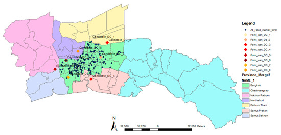 Figure 4. Point of main retail markets on ArcGIS software.
 - Demand for each retail market based on the population in each district with an average daily consumption of fresh fruits and vegetables in Thailand.
4.1.2. Operations of DC
We assumed the following operations in DCs for distributing fresh products:
- The demand for each delivery point must be satisfied by a vehicle assigned.
- Each vehicle leaves and returns to DC.
- The maximum vehicle capacity is 15 tons, according to the transportation regulation.
- The delivery time window starts from 2.00 a.m. and ends at 5.00 a.m.: retailers must prepare their products from 2.00 a.m.–5.00 a.m. every day. According to the regulation that trucks are not allowed to get in urban areas during working hours, the delivery time window should be satisfied.
- The speed of a truck from DC to the retailer is 10 km per hour (km/h): speed refers to the average of the worst congestion in the inner traffic congested road in Bangkok provided by the office of transport and traffic policy and planning, Thailand. To guarantee delivering goods in the event of unplanned circumstances within the time window, the speed of the truck was 10 km/h.
- Speed of a truck from wholesaler to DC is 30 km/h: each DC is located near a circulate road and highways.
- Service time for unloading fresh product to each retailer is 30 min.
4.2. Step II: Building Scenarios
The goal of this research was to find the optimal number and location of DCs to support the demand of retailers. In order to do this, eight possible scenarios were devised and summarized in Table 4. Scenario 1 assumes the existing distribution network. In addition, we propose three different approaches to select the location of distribution center. First, closest facility analysis was utilized to all eight available facilities in scenario 2. Second, in scenario 3, the number of facilities required to cover all demand points is minimized, which can be represented by n. Finally, we have utilized the approach for maximizing coverage which locates facilities where all demand points can be reached within a specified response time. By increasing the number of DCs which is secured from scenario 3 (n), we can design scenarios 4 to 8 represented by n + 1, n + 2, n + 3, n + 4 and n + 5, respectively. Even if the minimum number of DCs is equal to two, the maximum number of scenario using a maximize coverage approach should be equal to 7 (n + 5). Therefore, we can have at most eight scenarios. Each scenario will be explained in further detail.
Table 4.
Summary of building scenario.
- Scenario 1: Only one DC existing
Currently, each wholesaler delivers products to the existing DC. Then, retailers should pick up their products based on demand and deliver them to the retail market (see Figure 5).
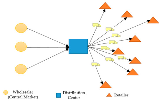
Figure 5.
The transport network of scenario 1 (AS IS).
Scenarios 2–8 were devised by assuming multi-location of DCs (see Figure 6) by locating new DCs and designing new transportation routes to reduce travel time and distance.
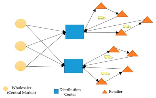
Figure 6.
The transport network of scenarios 2–8 (TO BE).
The details of the assumption to build scenarios 2–8 are described below.
- Scenario 2: Using all candidate DCs
The analysis assumed that all candidate DC should be addressed as a new facility. First, the closest facility in ArcGIS was used to assign 141 retailers to each DC. The delivery quantity to each retailer, delivery time window, and truck capacity were considered. Second, each DC delivered fresh fruits and vegetables to a group of retailers by using VRPTW analysis. Finally, LRP was used to find the total travel time and distance from wholesaler to DC.
- Scenario 3: From the result of minimizing the facility problem
In this scenario, we first found the minimum number of DCs required to cover all retailers using the location–allocation analysis. Then, retailers were assigned to possible candidate DCs within the impedance cutoff. Finally, the routes and schedules for distributing products from DCs were developed.
- Scenario 4 to Scenario 8: Using the maximize coverage problem
In Scenarios 4–8, we set the number of candidate DCs first. By increasing the number of candidate DCs from scenario 3 (minimizing the facility problem) to scenario 8 (the maximum number of DCs), we could extend the scenarios. Based on constraints in Table 4, maximizing coverage was used to choose the best set of candidate DCs, which could cover the maximum number of retailers within the impedance cutoff. Finally, the routes for delivery from selected DCs to 141 retailers were designed.
4.3. Step III: Scenario Analysis
Scenario analysis consisted of two phases, LAP and VRPTW. The two phases of scenario analysis are further detailed as follows:
- Phase I: LAP
In the first phase, from the set of candidate locations, the potential locations were selected and assign retailers to selected DCs. These were formulated by minimizing the number of locations and maximize coverage. The location–allocation analysis in ArcGIS network analyst tools starts by generating an origin–destination matrix by calculating the shortest-path costs. Then, it builds an edited version of the cost matrix, which can be obtained by generating a set semi randomized initial solutions, and it applies a vertex substitution heuristic to refine these solutions for creating a group of good solutions [35]. A metaheuristic combines the group of good solutions to create better solutions [35]. Finally, the metaheuristic returns the best solution with the current one when there is no additional significant improvement [35]. Therefore, the combination of an edited matrix, semi randomized initial solutions, a vertex substitution heuristic, and a refining metaheuristic can quickly yield the near-optimal results [35].
Moreover, both time and distance were specified as an impedance cutoff. The analysis assigned 141 delivery points (retailers) to candidate DCs. Moreover, the capacity of selected DCs was calculated to compare the balancing capacity of selected DCs for each scenario. Figure 7 shows an example of LAP in scenario 5 by maximizing coverage facility.
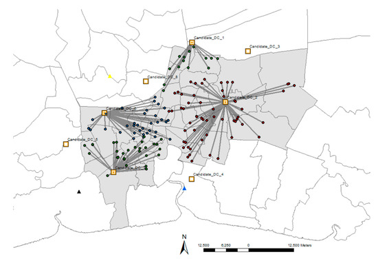
Figure 7.
Examples of location–allocation problem (LAP) in ArcGIS software (scenario 5).
- Phase II: VRPTW
In the second phase, the vehicle routing problem was solved using the locations of selected DC from phase I: LAP. The optimal vehicle routing was also obtained using ArcGIS network analyst tools based on a tabu search metaheuristic. It is designed for getting a solution very close to a global optimum in a general optimization problem [36]. The principle of a metaheuristic is to explore the search space composed of all feasible solutions in order to achieve the optimal solution that minimizes the objective function [37]. The tabu search is concerned with finding new and more effective ways of taking advantage of the mechanisms associated with both adaptive memory and responsive exploration [38].
In addition, both distance and time were used as impedances for all scenarios. The analysis focused on the vehicle routing from DC to the retailer and from wholesaler to retailer, the number of required trucks, total travel time, and total travel distance. In order to minimize total cost, we aimed to minimize the number of required trucks, total travel time, and total distance. In this research, all possible scenarios were implemented using ArcGIS; for example, Figure 8 shows the results of VRP in scenario 5, which optimized the route by using VRPTW.
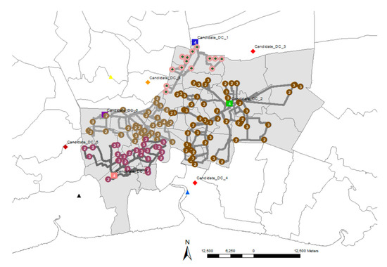
Figure 8.
Examples of vehicle routing problems with time window (VRPTW)in ArcGIS software (scenario 5).
4.4. Step IV: Performance Evaluation
In the last step, the indicators to measure the performance of each scenario were devised. In this research, we suggested quantitative indicators such as the number of DCs, the number of required trucks, total travel distance, and total travel time. However, the results of optimization showed that, while some truck drivers travel a long distance, others travel shorter distances. In this situation, the former truck drivers would be protesting and stop working because of the unbalanced assignment problem. Therefore, the indicator of fairness among drivers was developed with the standard deviation of travel time and the standard deviation of travel distance. At first, we compared all possible scenarios. Then, the performance of only alternative scenarios was compared with the relative score, as all quantitative indicators had different units. The results of the performance comparison helped to select better alternatives by considering practical constraints, such as budget and regulations.
5. Result and Discussion
5.1. Results of LAP and VRPTW
The results of the LAP of all scenarios are summarized in Table 5. The summary of VRPTW for all scenarios in terms of distance and time is presented in Table 6.
Table 5.
Summary of the results of the LAP analysis.
Table 6.
Summary of the results of the VRPTW analysis.
Regarding the VRPTW analysis, the results of the number of required trucks, total travel time, total travel distance, and fairness among drivers, scenarios 1 and 3 required 70 trucks, which is the minimum number trucks as compared to other scenarios. Although the number of required trucks in scenario 8 was higher than other scenarios, this scenario showed the best performance in terms of total travel time for 178.50 hr. Moreover, scenario 8 with 73 required trucks guaranteed the minimum total travel distance for 1109.12 km. However, scenario 7 showed the minimum value of the standard deviation of travel time (0.88) and distance (5.45). This means that scenario 7 guaranteed a better fairness among drivers and a well-balanced workload assignment.
In addition, Table 6 shows the improvement in terms of travel time and travel distance as compared to scenario 1. Scenario 8 showed the highest improvement percentage for both time (71.76%) and distance (72.92%). Therefore, scenario 8 showed the best performance for both total travel time and distance. Moreover, the best performance in terms of fairness among drivers was observed in scenario 7. For the number of required trucks, most alternative scenarios (except for scenario 3) showed a lower performance than that of scenario 1.
5.2. Comparison of the Resources and Required Capacity of DC
In order to build a new facility, it is necessary to consider the project and budget planning. To determine the number of DC, the number of required trucks, and the capacity of DC, all factors were related to the budget. Therefore, we examined two aspects to find insights for investment. First, we compared the number of DCs and the number of trucks to explore the relationship when the number of DC is changed. Second, through a comparison among the capacity of selected DCs, we were able to analyze the balancing capacity for each scenario.
The result of the LRP analysis concerning the number of DCs and the number of required trucks is reported in Figure 9. Scenario 1, with only one current DC, showed the highest performance in terms of the number of trucks (70). Even though scenario 8 required the biggest number of DCs (7 DC), it required only 73 trucks, which is similar to the minimum value, 70. Therefore, it can be concluded that scenario 8 did not require more trucks, even though the number of DC is increased.
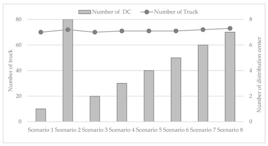
Figure 9.
The number of DCs and the number of trucks.
According to the results of VRPTW, all 141 retailers were covered by the number of trucks. Most drivers can supply only two retailers for a trip, as the capacity of the truck was limited. This is the main reason why the number of trucks for each scenario ranged from about 70 to 73. Therefore, the budget for the vehicle is quite similar for each scenario, so the budget for the building DCs was totally different based on the number of DC.
Figure 10 shows the required capacity of the selected DCs for each scenario. According to the assumption, all demand for retailers was allocated to the selected DCs. Therefore, the sum of the required capacity of the selected DCs was equal to the total demand. Considering the fixed cost or initial investment to build DCs for the fresh products, which was not relevant to the capacity, it is required to set the minimum level of required capacity for the selected DCs. Since this depended on several cost factors, the balance of the capacities among selected DCs should be investigated.
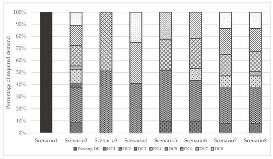
Figure 10.
Relative comparison of required capacity of DC.
In Figure 10, the scenarios with unbalanced capacity among the selected DCs can be clearly seen. For instance, the required capacities of DC_3 and DC_5 were considerably smaller than others in scenario 2. Likewise, scenarios 2 and 8 showed the unbalanced capacity among selected DCs. Scenarios 5, 6, and 7 were moderately shown in the unbalancing capacity. Therefore, to build a small DC as DC_3 and DC_5 in scenario 2 or DC_5 in scenario 8, it might be not worthwhile to invest. On the other hand, scenarios 3 and 4 showed well-balanced capacities. Therefore, it can be concluded that the balance of capacities could not be maintained with an increase in the number of DCs.
5.3. Comparison of Operations
Furthermore, fresh products logistics should also consider short travel time and distance from DC to retailers. Based on the results, Figure 11 shows the total travel time and distance from DCs to retailers for all scenarios.
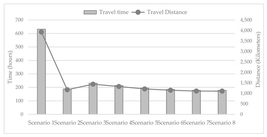
Figure 11.
Total travel time and total travel distance.
Scenario 1 showed the worst performance in terms of both total travel time and distance. It is clear that total travel time and distance of alternative scenarios can be dramatically decreased by adding more DCs and locating them where it is easy to access the highway. This is clear evidence for why we need to redesign the distribution network using multiple DCs, not only the biggest one, particularly in urban areas.
In this research, we suggested using a new indicator, fairness, which can be measured by the standard deviation of travel time and distance among drivers. Figure 12 shows the results of comparison among scenarios. By considering the fairness of traveling time and distance for each driver, scenario 1 showed the worst values of both time and distance. Similar to other indicators, alternative scenarios showed a considerably better performance in terms of fairness. Therefore, fairness among drivers improved with an increase in the number of DCs.
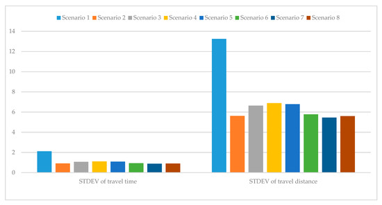
Figure 12.
The fairness index (standard deviation) of travel time and distance.
5.4. Overall Performance Evaluation
In addition, the performance of all possible scenarios should be evaluated by a joint consideration of the following six indicators (see Figure 13): the number of DCs, total travel time, total travel distance, standard deviation of travel distance, standard deviation of travel time, and number of required trucks. Given that all indicators have different units, we compared them with the relative score, which was obtained by dividing the score of scenarios with the maximum value among them.
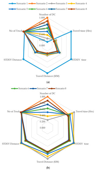
Figure 13.
(a) comparison with different indicators, all possible scenarios; (b) comparison with different indicators, only alternative scenarios.
Among eight scenarios, scenario 1 as the existing DC showed the worst performance in five indicators except for the number of DCs (see Figure 13a). Interestingly, even though we assumed a different number of DCs, the number of required trucks of all scenarios was almost identical. It is clear that alternative scenarios can guarantee a better performance in travel time, distance, and fairness among drivers as compared to scenario 1. Therefore, in order to choose the best scenario to apply to the practical transportation, we compared the performance among only alternative scenarios. The results are shown in Figure 13b.
In summary, the results can be interpreted in three aspects. First, when the budget of a new facility investment was considered to be a top priority, scenario 3 should be selected as the best one, as it requires the minimum level of resources, number of DCs (2 DCs), and the number of required trucks (70). However, due to the longer travel time and distance, scenario 3 was found to require more operating costs. Second, when the operating costs were considered as a top priority, scenario 8 had the best score of the total travel time and travel distance. Finally, scenario 7 showed the best score in terms of fairness among drivers based on STDEV of time and distance.
5.5. Distribution from Wholesaler to Selected DCs
In the current transportation system with only one DC, the wholesaler of each province (central market) delivers the products to DC based on demand. In this research, as in the current system, we assumed that the demand of each candidate DC was assigned to the nearest wholesaler. If the nearest wholesaler could not support the demand, another wholesaler would be selected to support the remained demand by considering the remained capacity of wholesaler and the distance from DC to the wholesaler. For example, in Figure 14, five candidate DCs in scenario 6 were supported by four wholesalers. Therefore, we should investigate and evaluate the performance of scenarios considering the distribution from wholesaler to selected DCs.
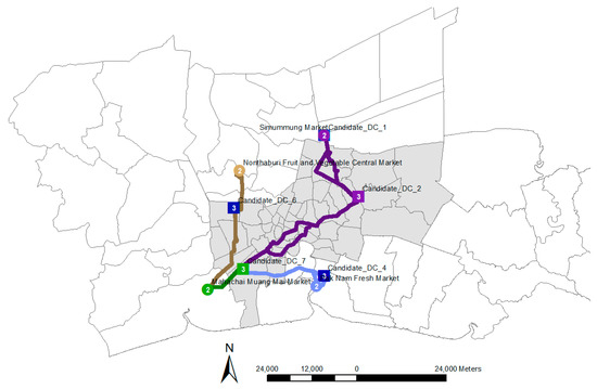
Figure 14.
Examples of location-routing problem (LRP) from wholesaler to DCs (scenario 6).
The results of LRP from wholesaler to the selected DCs of each scenario are summarized in Table 7. Similar to the results of the LRP analysis from DCs to retailers, scenario 1, which used only the existing DC, showed the worst performance, as all wholesalers should deliver their product to only single DC. Similarly, in scenario 3 with only two DCs, the performance was the worst among alternative scenarios. As the number of DCs increased, total travel time and distance tended to decrease. However, the biggest number of DCs could not guarantee the best performance. As it can be seen in Table 7, scenario 6 with five DCs showed the best performance with the shortest traveling distance and time among alternative scenarios.
Table 7.
Summary of distributions from the wholesale market to DCs.
5.6. Performance Evaluation of the Whole Distribution Network
The total travel time and distance from wholesaler to the retailer via DCs are shown in Table 8. In terms of total travel time, scenario 8 with seven DCs can be regarded as the best alternative. In the case of total travel distance, scenario 6 showed the best performance. However, scenario 5 with four DCs required the minimum number of trucks.
Table 8.
Summary of distribution from the wholesale market to the retail market.
It can be concluded that the proposed approach can guarantee a better performance to reduce travel time and distance as compared with the current existing distribution network. Reducing the number of vehicles, travel distance and travel time lead to reduction in distribution cost and greenhouse gas [17,39]. One of the alternative scenarios can be suggested to build the practical network by considering several different factors such as the triple bottom line from the definition of sustainability, economic, social, and environmental values.
For instance, the economic benefit will increase with a decrease of the total time and distance, which can reduce operating costs, like fuel costs. At the same time, environmental benefits can be increased because it can reduce energy consumption and emission in an urban area. Finally, fairness may represent a social value, as it implies the balance of the assigned task or workload among drivers.
Specifically, sustainability can be achieved by considering the following factors to design urban distribution network to simultaneously enhance the economic, social, and environmental values:
- Economic and environmental factor (Viable): Number of trucks (delivering the products to make money vs. exhaust emission)
- Economic and social factor (Equitable): Number of DCs (fixed cost vs. increasing product access and job opportunity), fairness among drivers, both time and distance (operation cost vs. improving worker’s rights)
- Environment and social factor (Bearable): Total distance and total time (saving energy and emission vs. avoiding food spoilage and foodborne diseases), number of DCs (access to fresher food vs. increasing the quality of life)
5.7. Sensitivity Analysis
The procedure and result of sensitivity analysis are presented in this section in order to verify the validity of the results. Generally, the sensitivity analysis is required to build more robust models considering variable demand and capacity of DC in daily operations. The objective of sensitivity analysis is to monitor the changes of the result of LAP and VRPTW analysis when demand is increasing by 120%, 150%, and 200%, respectively. To verify the robustness of the results obtained with closest facility, minimize facility, and maximize coverage model, we conduct the LAP and VRPTW analysis by using maximized capacitated coverage, which the capacity of DC is limited. The maximum storage capacity of each DC is determined in Table 9.
Table 9.
Maximum storage capacity.
In Table 10, the results of the LAP analysis according to the increased demand of fresh fruits and vegetables are shown. We conduct a sensitivity analysis by repeating all the computational experiments for all eight scenarios. We compared the result of LAP between Table 5 and Table 10 when considering the increased demand. As it can be found from the result, the number of selected DCs is not changed, but some of the DCs are substituted by others as the demand increases, which is illustrated by being bold and underlined. For scenario 3, the DC_6 was substituted by the DC_7 and DC_5 in scenario 3. The DC_4 was chosen as the demand increase in scenario 4. In the case of scenario 5, the DC_4 and DC_8 were selected when demand increased by 150% and 200%. In scenario 6, the DC_8 was chosen for replacing the DC_1 when demand increased 150% and 200%.
Table 10.
Summary of the results of the LAP analysis when determined maximum storage capacity.
According to the results of the LAP analysis, the performance indicators of the selected network for each scenario are assessed by using VRPTW analysis. Like LAP analysis, the changes of all indicators have been analyzed while the demand increases by 120%, 150%, and 200%, respectively. The results of the sensitivity analysis are summarized in Table 11 in terms of different indicators. It can be said that there exists a significant difference in the number of required trucks, travel time, and travel distance. These numbers seem to increase slightly when the demand increases by 120%. However, when the demand increases by as much as 150%, and 200%, a significant increase in terms of these indicators exists, even though they look like having a proportional relationship with the demand.
Table 11.
Summary of sensitivity analysis.
In conclusion, it can be indicated that the results of the original LAP and VRPTW are still robust when demand increases by 120%. In addition, the results of sensitivity analysis verify that the alternative scenarios show the better performance when compared with the current distribution network if the demand of fresh fruits and vegetables increases.
6. Conclusions
A cold chain for perishable foods aims to maintain the food safety and quality of the products under temperature monitoring and control. Transportation and distribution within delivery time windows become a challenge for the fresh food management. With urban population growth and increasing traffic congestion issues, a major existing DC may inefficiently meet customer requirements. To support the increasing demand and improve the quality of life in Bangkok metropolitan, an advanced transportation and distribution network for fresh products is needed.
This research aimed to design a transportation network for fresh fruit and vegetables considering total travel time, total travel distance, and fairness among drivers by integrating LAP and VRPTW analysis. In addition, the results of LRP were obtained based on the actual location of origin, destination, and candidate DCs. Furthermore, candidate DCs were selected by minimizing facility location and maximizing coverage approach. All possible scenarios were devised and compared in terms of their performance based on six quantitative indicators: the number of the DCs, total travel distance, total travel time, the standard deviation of travel distance, and travel time, which refers to fairness among drivers, as well as the number of required trucks.
The results highlight that the alternative scenarios based on mathematical models can guarantee a significantly improved performance, such as total travel time, total travel distance, and fairness than the current distribution network. For instance, when considering total travel time and distance from wholesaler to retailer via DCs, scenario 8 with seven DCs showed the best performance in travel time, while scenario 6 with five DCs showed the shortest distance. In terms of fairness, scenario 7 with six DCs may be regarded as the best alternative with the highest fairness indicator among drivers in both traveling time and distance. In addition, the results of performance evaluation may help the network designer consider and select a better scenario. Comparing makes it possible to enhance and balance economic, environmental, and social values to achieve sustainability in urban distribution. In order to consider the balance of the assigned workload in this research, we designed the fairness indicator based on the standard deviation of traveling distance and time across drivers.
There are several methods to extend this research that can be suggested as future research directions. First, in order to make the problem simple without a loss of generalizability of our results, we did not specify the capacity of each DC at the beginning of the study. However, it may be helpful to design and develop a flexible transportation network. Second, it is difficult to forecast the demand for fresh fruit and vegetables from each retailer in Bangkok city. The demand for fresh fruit and vegetables was calculated based on the average consumption per year and the population of each district in Bangkok. The current results may be improved by securing the category and practical demand for fresh products from the retailer. Third, we have applied to the fixed average speed of outside and inside of the Bangkok area for solving VRPTW. However, the speed of trucks will be different according to the traffic status. Therefore, after securing the actual average speed of all roads, it is possible to elaborate the result of this research. Fourth, there is not enough information and data about land price, construction cost, and operating cost in fresh food DC. Therefore, the investment cost and operating cost should be calculated in future research. Fifth, the fresh products logistics operations should be developed using advanced techniques when it needs more accuracy. The optimization and machine learning should be applied to solve complex problems. Finally, the discrepancy in priority setting and information sharing among parties should be a focus.
Author Contributions
Conceptualization, J.S. and K.S.S.; Methodology, J.S.; Software, J.S.; Validation, J.S. and K.S.S.; Formal Analysis, J.S. and K.S.S.; Investigation, J.S.; Resources, J.S.; Data Curation, J.S.; Writing-Original Draft Preparation, J.S.; Writing-Review & Editing, K.S.S.; Visualization, J.S.; Supervision, K.S.S.
Funding
This work was supported by the University of Incheon Research Grant in 2014.
Conflicts of Interest
The authors declare no conflict of interest.
References
- Shashi, K.; Cerchione, R.; Singh, R.; Centobelli, P.; Shabani, A. Food cold chain management: From a structured literature review to a conceptual framework and research agenda. Int. J. Logist. Manag. 2018, 29, 792–821. [Google Scholar]
- Mejjaouli, S.; Babiceanu, R.F. Cold supply chain logistics: System optimization for real-time rerouting transportation solutions. Comput. Ind. 2018, 95, 68–80. [Google Scholar] [CrossRef]
- Hsiao, Y.H.; Chen, M.C.; Chin, C.L. Distribution planning for perishable foods in cold chains with quality concerns: Formulation and solution procedure. Trends Food Sci. Technol. 2017, 61, 80–93. [Google Scholar] [CrossRef]
- Kuo, J.C.; Chen, M.C. Developing an advanced Multi-Temperature Joint Distribution System for the food cold chain. Food Control 2010, 21, 559–566. [Google Scholar] [CrossRef]
- Hsu, C.I.; Chen, W.T. Optimizing fleet size and delivery scheduling for multi-temperature food distribution. Appl. Math. Model. 2014, 38, 1077–1091. [Google Scholar] [CrossRef]
- CITY POPULATION. Available online: https://www.citypopulation.de/php/thailand-prov-admin.php?adm1id=B (accessed on 5 April 2018).
- Nirattiwongsakorn, P. Congestion in Bangkok And Lessons from London and Singapore. Available online: https://phannisan.files.wordpress.com/2016/05/phannisa_congestion-in-bangkok.pdf (accessed on 10 April 2018).
- TOMTOM TRAFFIC INDEX. Available online: https://www.tomtom.com/en_gb/trafficindex/list?citySize=LARGE&continent=ALL&country=ALL (accessed on 5 April 2018).
- Bangkokpost. Average Morning Rush-Hour Speed Slows to 15 kph. Available online: https://www.bangkokpost.com/news/transport/807204/rush-hour-gets-slower-still (accessed on 5 April 2018).
- Wang, Y.; Ma, X.; Wang, Y.; Mao, H.; Zhang, Y. Location optimization of multiple distribution centers under fuzzy environment. J. Zhejiang Univ. Sci. A 2012, 13, 782–798. [Google Scholar] [CrossRef]
- Yang, L.; Ji, X.; Gao, Z.; Li, K. Logistics distribution centers location problem and algorithm under fuzzy environment. J. Comput. Appl. Math. 2007, 208, 303–315. [Google Scholar] [CrossRef]
- Govindan, K.; Jafarian, A.; Khodaverdi, R.; Devika, K. Two-echelon multiple-vehicle location-routing problem with time windows for optimization of sustainable supply chain network of perishable food. Int. J. Prod. Econ. 2014, 152, 9–28. [Google Scholar] [CrossRef]
- Aramyan, L.H.; Lansink, A.G.J.M.O.; Van Der Vorst, J.G.A.J.; Van Kooten, O. Performance measurement in agri-food supply chains: A case study. Supply Chain Manag. 2007, 12, 304–315. [Google Scholar] [CrossRef]
- Wang, G.; Gunasekaran, A.; Ngai, E.W.T. Distribution network design with big data: Model and analysis. Ann. Oper. Res. 2018, 270, 539–551. [Google Scholar] [CrossRef]
- Singh, A.K.; Subramanian, N.; Pawar, K.S.; Bai, R. Cold chain configuration design: Location-allocation decision-making using coordination, value deterioration, and big data approximation. Ann. Oper. Res. 2018, 270, 433–457. [Google Scholar] [CrossRef]
- Gallo, A.; Accorsi, R.; Baruffaldi, G.; Manzini, R. Designing sustainable cold chains for long-range food distribution: Energy-effective corridors on the Silk Road Belt. Sustainable 2017, 9, 2044. [Google Scholar] [CrossRef]
- Bosona, T.; Nordmark, I.; Gebresenbet, G.; Ljungberg, D. GIS-Based Analysis of Integrated Food Distribution Network in Local Food Supply Chain. Int. J. Bus. Manag. 2013, 8, 13. [Google Scholar] [CrossRef]
- Bozkaya, B.; Yanik, S.; Balcisoy, S. A GIS-based optimization framework for competitive multi-facility location-routing problem. Netw. Spat. Econ. 2010, 10, 297–320. [Google Scholar] [CrossRef]
- Bosona, T.; Gebresenbet, G.; Nordmark, I.; Ljungberg, D. Integrated Logistics Network for the Supply Chain of Locally Produced Food, Part I: Location and Route Optimization Analyses. J. Serv. Sci. Manag. 2011, 4, 174–183. [Google Scholar] [CrossRef]
- Hsiao, Y.H.; Chen, M.C.; Lu, K.Y.; Chin, C.L. Last-mile distribution planning for fruit-and-vegetable cold chains. Int. J. Logist. Manag. 2018, 29, 862–886. [Google Scholar] [CrossRef]
- Hsu, C.I.; Liu, K.P. A model for facilities planning for multi-temperature joint distribution system. Food Control 2011, 22, 1873–1882. [Google Scholar] [CrossRef]
- Marianov, V.; Serra, D. Location Problems in the Public Sector. In Facility Location: Applications and Theory; Springer: Berlin/Heidelberg, Germany, 2002. [Google Scholar]
- Wang, S.; Tao, F.; Shi, Y. Optimization of location–routing problem for coldchain logistics considering carbon footprint. Int. J. Environ. Res. Public Health 2018, 15, 86. [Google Scholar] [CrossRef]
- Fazayeli, S.; Eydi, A.; Kamalabadi, I.N. Location-routing problem in multimodal transportation network with time windows and fuzzy demands: Presenting a two-part genetic algorithm. Comput. Ind. Eng. 2018, 119, 233–246. [Google Scholar] [CrossRef]
- Ma, Z.J.; Wu, Y.; Dai, Y. A combined order selection and time-dependent vehicle routing problem with time widows for perishable product delivery. Comput. Ind. Eng. 2017, 114, 101–113. [Google Scholar] [CrossRef]
- Solak, S.; Scherrer, C.; Ghoniem, A. The stop-and-drop problem in nonprofit food distribution networks. Ann. Oper. Res. 2014, 221, 407–426. [Google Scholar] [CrossRef]
- Musolino, G.; Polimeni, A.; Vitetta, A. Freight vehicle routing with reliable link travel times: A method based on network fundamental diagram. Transp. Lett. 2016, 10, 159–171. [Google Scholar] [CrossRef]
- Musolino, G.; Rindone, C.; Polimeni, A.; Vitetta, A. Planning urban distribution center location with variable restocking demand scenarios: General methodology and testing in a medium-size town. Transp. Policy 2019, 80, 157–166. [Google Scholar] [CrossRef]
- ESRI. Types of Network Analysis Layers. Available online: http://desktop.arcgis.com/en/arcmap/latest/extensions/network-analyst/types-of-network-analyses.htm (accessed on 10 April 2018).
- ESRI. Location-Allocation Analysis. Available online: http://desktop.arcgis.com/en/arcmap/10.4/extensions/network-analyst/location-allocation.htm (accessed on 10 April 2018).
- ESRI. Vehicle routing Problem Analysis. Available online: http://desktop.arcgis.com/en/arcmap/10.4/extensions/network-analyst/vehicle-routing-problem.htm#GUID-2E0981B2-B20B-4A38-88A8-94B15DA2A5B7 (accessed on 10 April 2018).
- Kallehauge, B.; Larsen, J.; Oli, B.G.; Madsen, M.M.S. Vehicle Routing Problem with Time Windows. In Column Generation; GERAD 25th Anniversary Series; Springer: New York, NY, USA, 2005; pp. 67–98. [Google Scholar]
- Office of the National Economic and Social Development Council. Thailand’s Logistics Development Strategy (2017–2021). Available online: http://www.nesdb.go.th/download/document/logistic/plan3.pdf (accessed on 15 April 2019).
- Ministry of Agriculture and Cooperatives. Thailand’s Agricultural Development Plan (2017–2021). Available online: http://tarr.arda.or.th/static2/docs/development_plan2559.pdf (accessed on 15 April 2019).
- ESRI. Algorithms Used by the ArcGIS Network Analyst Extension. Available online: https://desktop.arcgis.com/en/arcmap/latest/extensions/network-analyst/algorithms-used-by-network-analyst.htm (accessed on 10 April 2018).
- Hertz, A.; de Werra, D. The tabu search metaheuristic: How we used it. Ann. Math. Artif. Intell. 1990, 1, 111–121. [Google Scholar] [CrossRef]
- Jemai, M.; Dimassi, S.; Ouni, B.; Mtibaa, A. A metaheuristic based on the tabu search for hardware-software partitioning. Turkish J. Electr. Eng. Comput. Sci. 2017, 901–912. [Google Scholar] [CrossRef]
- Glover, F.; Laguna, M. Tabu Search; Kluwer Academic Publishers: Norwell, MA, USA, 1997. [Google Scholar]
- Ljungberg, D.; Gebresenbet, G.; Aradom, S. Logistics Chain of Animal Transport and Abattoir Operations. Biosyst. Eng. 2007, 96, 267–277. [Google Scholar] [CrossRef]
© 2019 by the authors. Licensee MDPI, Basel, Switzerland. This article is an open access article distributed under the terms and conditions of the Creative Commons Attribution (CC BY) license (http://creativecommons.org/licenses/by/4.0/).