A Kinematic Controller for Liquid Pouring between Vessels Modelled with Smoothed Particle Hydrodynamics


Abstract
:Featured Application
Abstract
1. Introduction
2. Fluid Models
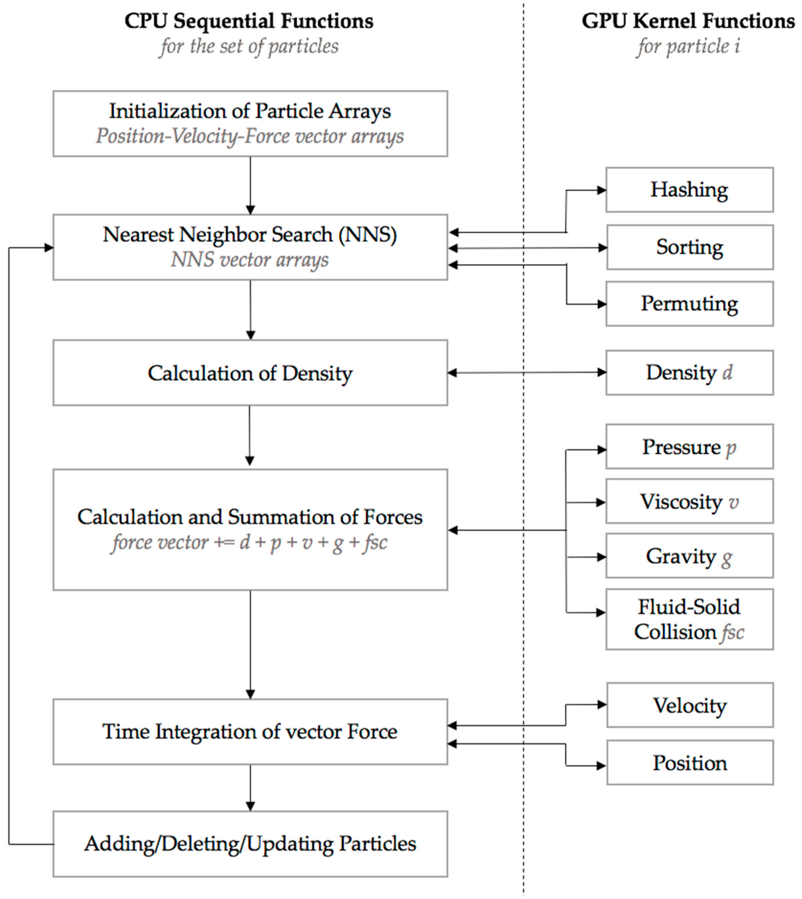
2.1. SPH Model
2.2. Free Fall Model
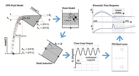
3. Modelling and Control
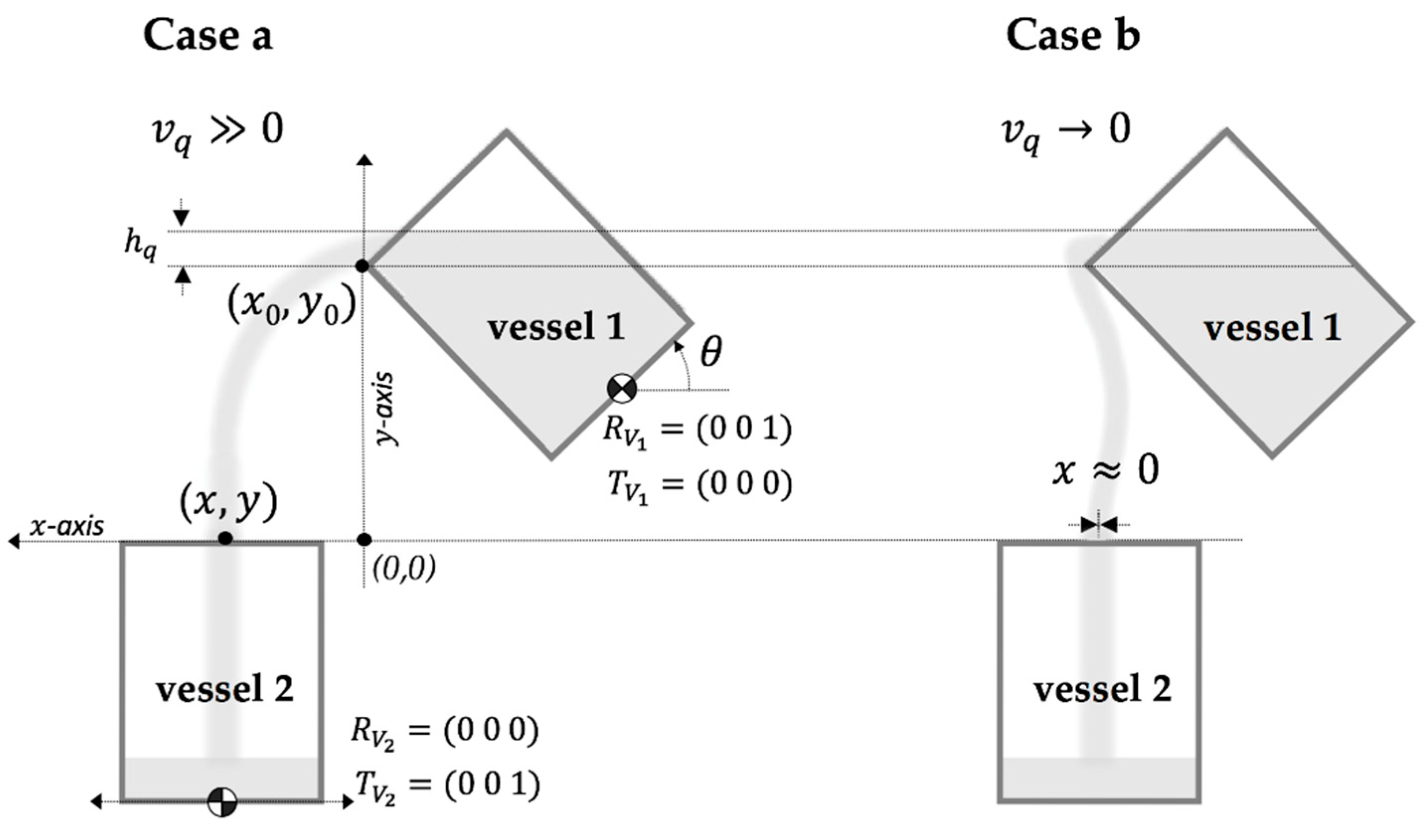
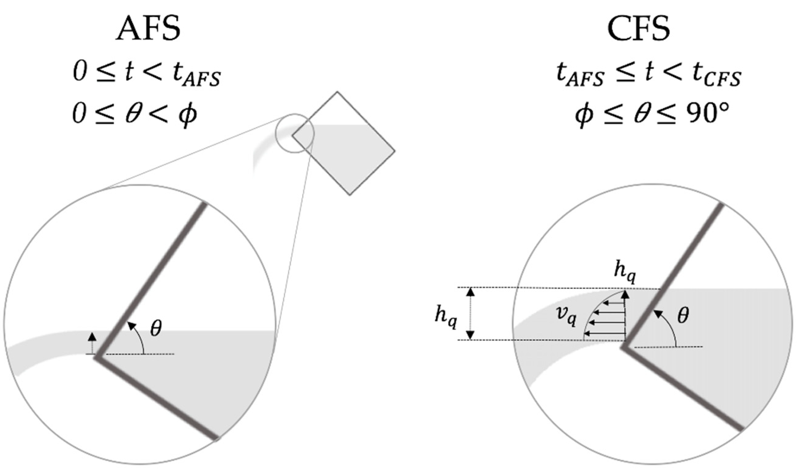
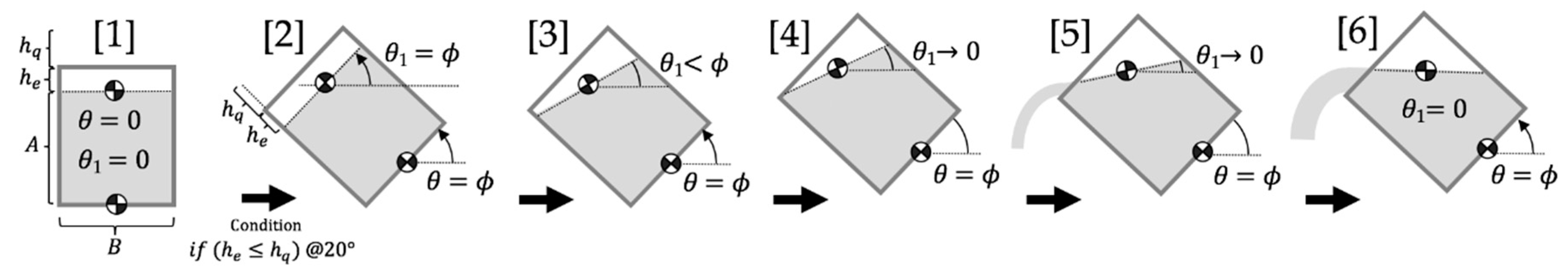
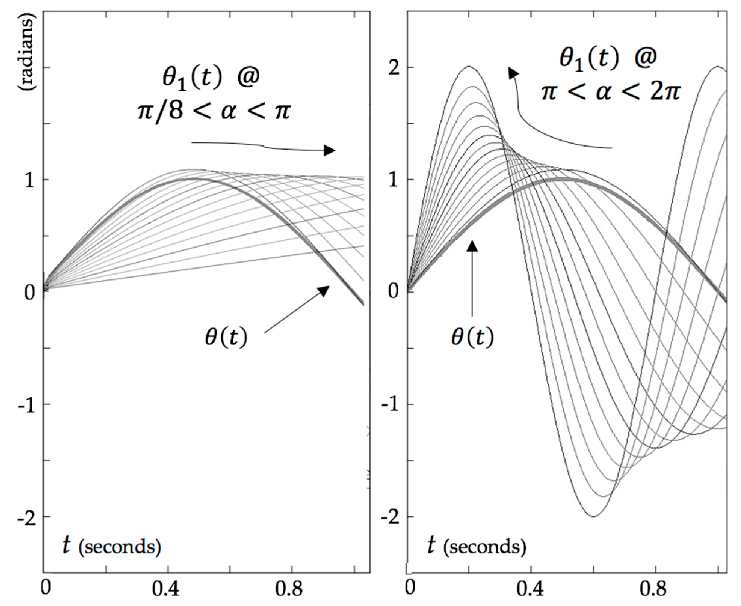
3.1. Approaching Flow Stage (AFS)
3.2. Constant Flow Stage (CFS)
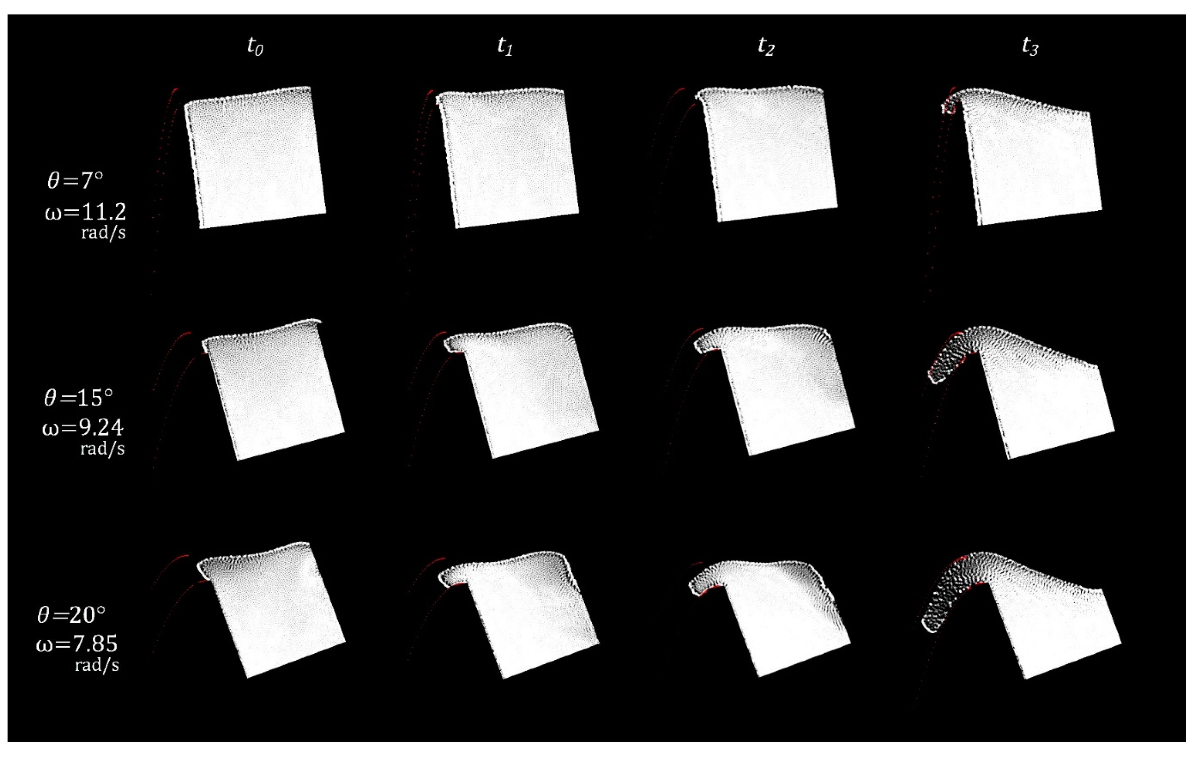
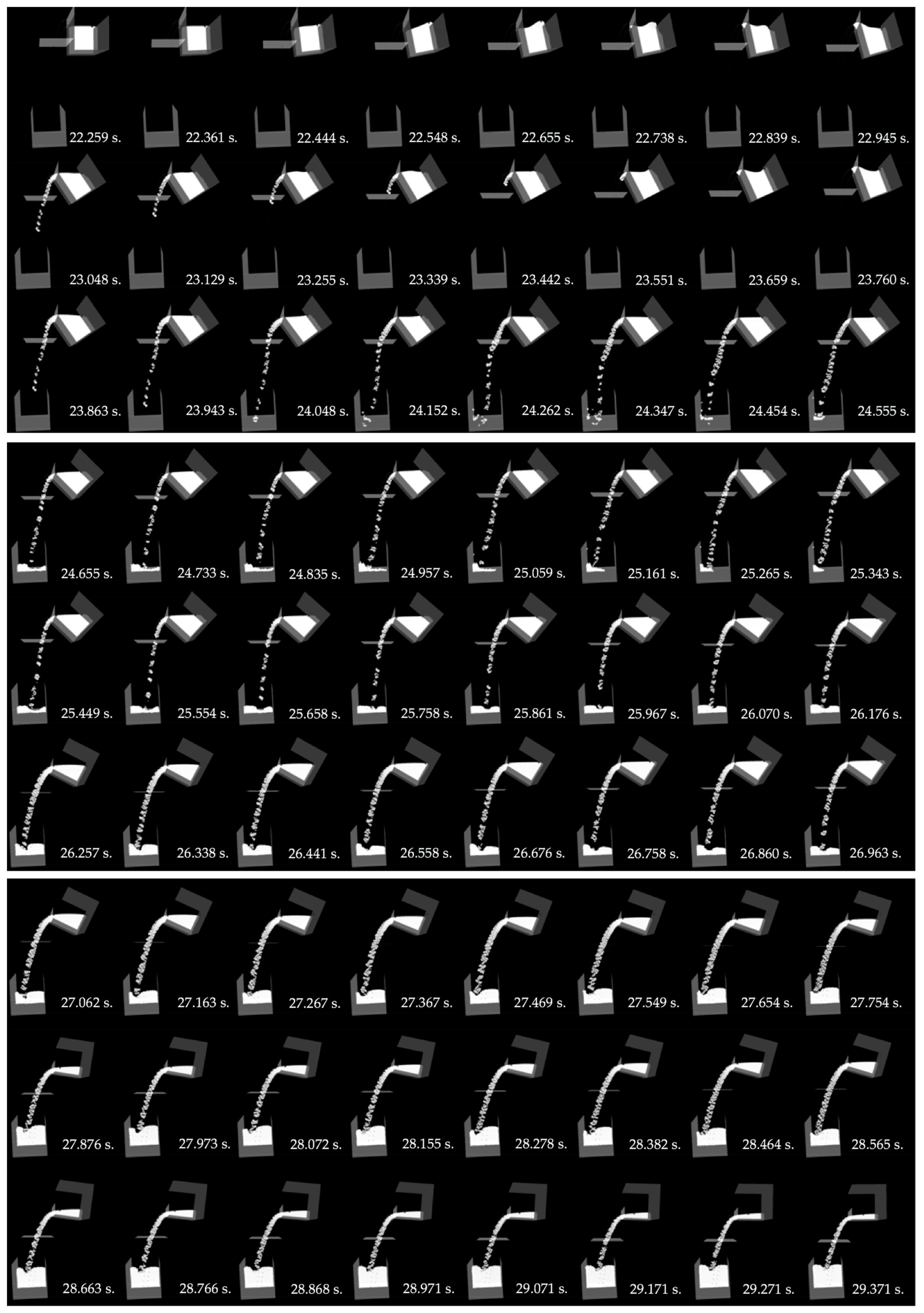
4. Results and Discussion
5. Conclusions
Supplementary Materials
Author Contributions
Funding
Conflicts of Interest
Abbreviations
| SPH | smoothed particle hydrodynamics |
| GPU | graphic processing unit |
| SIM | slosh induction method |
| NSS | nearest neighbor search |
| CFS | constant flow stage |
| AFS | approaching flow stage |
| STF | system transfer function |
| PID | proportional, integral and derivative |
Nomenclature
| velocity and height of the outflow | at vessel 1 pouring tip | ||
| empty space height in vessel 1 | rotation angle of vessel 1 | ||
| density and mass of particle i | free surface rotation angle in vessel 1 | ||
| velocity and pressure of particle i | conditional angle of | ||
| function of interpolation or SPH kernel | ending time for AFS | ||
| vector distance between particle i and j | ending time for CFS | ||
| SPH smoothing length | height of vessel 1 | ||
| pressure force of i | base length (inside width) of vessel 1 | ||
| viscosity force of i | height, mass and moment of inertia of the rigid model | ||
| gravity force | height, pendulum distance, mass and angle of the nth pendulum | ||
| gradient of | proportional, integral and derivative constants | ||
| laplacian of | laplace variable | ||
| rest density of water | plant gain and controller gain | ||
| speed of sound | CFS vectors | ||
| Tait’s equation constant | linear step mode of | ||
| location of the outflow trajectory fall | Frequency of the slosh | ||
| location of the outflow tip in vessel 1 | time variable | ||
| dynamic viscosity |
Appendix A
Appendix B
References
- Davis, E. Pouring Liquids: A Study in Commonsense Physical Reasoning. Artif. Intell. 2008, 172, 1540–1578. [Google Scholar] [CrossRef]
- Dey, S. Free Overflow in Open Channels: State-of-the-art review. Flow Meas. Instrum. 2002, 13, 247–264. [Google Scholar] [CrossRef]
- Bauer, S.W. The Free Overfall as a Flow Measurement Device. Master’s Thesis, Lehigh University, Bethlehem, PA, USA, June 1970. [Google Scholar]
- He, J.; Chen, X.; Wang, Z.; Cao, C.; Yan, H.; Peng, Q. Real-time adaptive fluid simulation with complex boundaries. Visual Comput. 2010, 26, 243–252. [Google Scholar] [CrossRef]
- Hirt, C.W.; Nichols, B.D. A Volume of Fluid (VOF) Method for the Dynamics of Free Boundaries. J. Comput. Phys. 1981, 39, 201–225. [Google Scholar] [CrossRef]
- Becker, M.; Teschner, M. Weakly compressible SPH for free surface flows. In Proceedings of the 2007 ACM SIGGRAPH/Eurographics Symposium on Computer Animation, San Diego, CA, USA, 2–4 August 2007; pp. 1–8. [Google Scholar]
- Shao, S.; Lo, E. Incompressible SPH method for simulating Newtonian and non-Newtonian flows with free surface. Adv. Water Resour. 2003, 27, 787–800. [Google Scholar] [CrossRef]
- Pan, Z.; Park, C.; Manocha, D. Robot Motion Planning for Pouring Liquids. In Proceedings of the 26th International Conference on Automated Planning and Scheduling, London, UK, 12–17 June 2016; pp. 518–526. [Google Scholar]
- Lopez-Guevara, T.; Taylor, N.; Gutmann, M.; Ramamoorthy, S.; Subr, K. Adaptable Pouring: Teaching robots not to spill using fast but approximate fluid simulation. In Proceedings of the 1st Conference on Robot Learning, Mountain View, CA, USA, 13–15 November 2017; pp. 77–86. [Google Scholar]
- Schenck, C.; Fox, D. Visual Closed-Loop Control for Pouring Liquids. In Proceedings of the IEEE International Conference on Robotics and Automation, Singapore, 29 May–3 June 2017; pp. 2629–2636. [Google Scholar]
- Langsfeld, J.D.; Kaipa, K.N.; Gentili, R.J.; Reggia, J.A.; Gupta, S.K. Incorporating failure-to-success transitions in imitation learning for a dynamic pouring task. In Proceedings of the IEEE International Conference on Intelligent Robots and Systems, Workshop on Compliant Manipulation: Challenges and Control, Chicago, IL, USA, 14–18 September 2014. [Google Scholar]
- Ito, A.; Noda, Y.; Terashima, K. Outflow Liquid Falling Position Control by Considering Lower Ladle Position and Clash Avoidance with Mold. In Proceedings of the 3rd IFAC Workshop on Automation in the Mining, Mineral, and Metal Industries, Gifu, Japan, 10–12 September 2012; pp. 240–245. [Google Scholar]
- Grundelius, M. Methods for Control of Liquid Slosh. Ph.D. Thesis, Lund University, Lund, Sweden, October 2001. [Google Scholar]
- Goffin, L.; Erpicum, S.; Dewals, B.; Pirotton, M.; Archambeau, P. Validation of a SPH Model for Free Surface Flows. In Proceedings of the SimHydro: Modelling of Rapid Transitory Flows, Sophia Antipolis, Nice, France, 11–13 June 2014. [Google Scholar]
- Krog, O.E.; Elster, A.C. Fast GPU-based Fluid Simulations Using SPH. In Proceedings of the 10th International Conference on Applied Parallel and Scientific Computing, Reykjavik, Iceland, 6–9 June 2010; pp. 98–109. [Google Scholar]
- OpenGL Site. Available online: www.opengl.org (accessed on 23 September 2019).
- The OpenGL Utility Toolkit GLUT Site. Available online: www.opengl.org/resources/libraries/glut/ (accessed on 23 September 2019).
- OpenCL Community Site. Available online: www.opencl.org (accessed on 23 September 2019).
- NVIDIA. OpenCL Sorting Networks. Available online: http://developer.download.nvidia.com/compute/cuda/4_2/rel/sdk/website/OpenCL/html/samples.html (accessed on 23 September 2019).
- Harada, T.; Koshizuka, S.; Kawaguchi, Y. Smoothed Particle Hydrodynamics on GPUs. In Proceedings of the 5th International Conference on Computer Graphics, Petropolis, Brazil, 30 May–2 June 2007; pp. 63–70. [Google Scholar]
- Liu, G.R.; Liu, M.B. Smoothed Particle Hydrodynamics, A meshfree particle method, 1st ed.; World Scientific Publishing Company: Toh Tuck, Singapore, 2003; pp. 123–124. [Google Scholar]
- Monaghan, J. Simulating Free Surface flows with SPH. J. Comput. Phys. 1994, 110, 399–406. [Google Scholar] [CrossRef]
- Ericson, C. Real–Time Collision Detection, 1st ed.; Morgan Kaufmann Publishers: San Francisco, CA, USA, 2004; pp. 175–190. [Google Scholar]
- Cossins, P.J. Smoothed Particle Hidrodynamics (Chapter 3: Smoothed Particle Hydrodynamics). Ph.D. Thesis, University of Leicester, Leicester, UK, 2010. [Google Scholar]
- Bell, N.; Yun, Y.; Mucha, P.J. Particle-based simulation of granular materials. In Proceedings of the 2005 ACM SIGGRAPH/Eurographics Symposium on Computer Animation, Los Angeles, CA, USA, 29–31 July 2005; pp. 77–86. [Google Scholar]
- Raju, K.; Asawa, G. Viscosity and Surface Tension effects on Weir Flow. J. Hydraul. Div. 1977, 103, 1227–1231. [Google Scholar]
- Lee, G.J. Moment of inertia of liquid in a tank. Int. J. Nav. Archit. Ocean Eng. 2014, 6, 132–150. [Google Scholar] [CrossRef]
- Abramson, H.N. NASA SP-106 Report: The Dynamic Behavior of Liquids in Moving Containers; NASA: Washington, DC, USA, 1966.
- Ibrahim, R. Liquid Sloshing Dynamics Theory and Applications, 1st ed.; Cambridge University Press: New York, NY, USA, 2005. [Google Scholar]
- Roberts, J.R.; Basurto, E.R.; Chen, P.-Y. NASA CR-406 Report: Slosh Design Handbook; NASA: Washington, DC, USA, 1966.
- Liu, M.; Shao, J.; Chang, J. On the treatment of solid boundary in Smoothed Particle Hydrodynamics. Sci. China Technol. Sci. 2012, 55, 244–254. [Google Scholar] [CrossRef]


© 2019 by the authors. Licensee MDPI, Basel, Switzerland. This article is an open access article distributed under the terms and conditions of the Creative Commons Attribution (CC BY) license (http://creativecommons.org/licenses/by/4.0/).
Share and Cite
Camporredondo, G.; Barber, R.; Legrand, M.; Muñoz, L. A Kinematic Controller for Liquid Pouring between Vessels Modelled with Smoothed Particle Hydrodynamics. Appl. Sci. 2019, 9, 5007. https://doi.org/10.3390/app9235007
Camporredondo G, Barber R, Legrand M, Muñoz L. A Kinematic Controller for Liquid Pouring between Vessels Modelled with Smoothed Particle Hydrodynamics. Applied Sciences. 2019; 9(23):5007. https://doi.org/10.3390/app9235007
Chicago/Turabian StyleCamporredondo, Gabriel, Ramón Barber, Mathieu Legrand, and Lourdes Muñoz. 2019. "A Kinematic Controller for Liquid Pouring between Vessels Modelled with Smoothed Particle Hydrodynamics" Applied Sciences 9, no. 23: 5007. https://doi.org/10.3390/app9235007
APA StyleCamporredondo, G., Barber, R., Legrand, M., & Muñoz, L. (2019). A Kinematic Controller for Liquid Pouring between Vessels Modelled with Smoothed Particle Hydrodynamics. Applied Sciences, 9(23), 5007. https://doi.org/10.3390/app9235007