Investigation on Single Tube CFST Arch Models by Modeling Structural Stressing State Based on NSF Method

Abstract

This paper investigated the behavioral characteristics of two single tube concrete-filled steel tube (CFST) arch models under different loads. Applying the numerical shape function (NSF) method, the limited strain data of arch models were interpolated to obtain more detailed strain information at unmeasured points. By numerically modeling and characterizing the structural stressing state of arches, these interpolated strains were calculated as the normalized strain energy density (SED) sum to plot the corresponding characteristic curves. Utilizing the Mann-Kendall (M-K) criterion, the qualitative characteristic load was detected from the curve and was referred to as the failure load, updating the existing definition of structural failure. Then, from the perspective of experimental strains, strain/stress fields, and stressing state submodes of internal forces obtained based on the NSF method, the working behavioral characteristics of each respective CFST arch model under loads were embodied in detail. The mutation features were distinguished from the development trend of strain/stress fields or distribution patterns of internal forces to verify the rationality of the updated failure load. Consequently, the NSF method can have a reasonable interpolation on the limited experimental data. By modeling structural stressing state, it can conduct an accurate estimation of the structural failure load and provide a reference for the future design of arch bridges.

1. Introduction

Over the past few decades, the prevalence of concrete-filled steel tube (CFST) arches has steadily increased in the construction industry and bridge engineering, especially in large-span roofs and bridges. The application of CFST arches owes to their strong bearing capacity, large span potential, beautiful appearance, and convenient construction [1,2]. Also, as a composite structure, the CFST arches can enhance structural performance by fully utilizing the compressive and tensile strengths of steel and concrete, respectively, which greatly promotes the usage efficiency of materials [3]. In China, it has been roughly estimated that more than 400 CFST arch bridges have been built, and the largest span is over 500 m [4,5]. Among these various structure forms of CFST arches, single tube CFST arches make up a large proportion in small- and medium-span bridge constructions. Compared to arches with other types of cross-sections, such as dumbbell-shaped sections and truss sections, single tube CFST arches have simpler structural forms and mechanical behaviors.

However, to date, the extensive use of single tube CFST arches has not led to deeper studies on their working behaviors. Theoretical and experimental research about arches has simply involved a calculating method, bearing capacity under in-plane loads or spatial loads [6,7], and dynamic performance [8,9], inclusive of considering the effects of initial stress [10] and initial imperfection, geometric and material nonlinearity, et al. [11,12,13]. Chen [14] conducted a model experiment of two CFST rib arches under in-plane loads and found that they have outstanding ductility and bearing properties. Liu et al. [15] used the finite element program to study the ultimate load-bearing capacity of long-span CFST arch bridges with fly-bird-type and the results indicated that the effect of both geometric and material nonlinearity could not be neglected. Using a CFST arch bridge with a span of 80 m, for example, Han et al. [16] studied its stability using the general finite element program. Deng et al. [17] proposed a co-rotational formulation in the setting of finite elements for three-dimensional nonlinear analysis of the ultimate bearing capacity of a circular (CFST) arch, considering both geometric and material nonlinearities. Liu et al. [18] tested six fixed CFST parabolic arches to study the effects of the rise-span ratio and the non-uniform moment. Wang et al. [19] analyzed the out-plane elastic stability of typical single tube CFST arch bridges using the finite element method and provided a calculation method.

From the literature above, the lack of sufficient large-scale experiments on single tube CFST arches to investigate their complex in-plane or out-plane working behaviors and failure mechanisms can be seen. In existing experimental analysis, the measured strain data has always not been fully utilized, leading to the neglect of extensive unseen information of structural working behavior characteristics, which could have been extracted from experimental strain data using the appropriate methods. Using the finite element (FE) method, the mechanics performance of structures will have greater clarities. Inevitably, the finite element model is often simplified or assumed by researchers with experience in structural design. The problem arises that the calculation results of structural responses using these simplified models always have deviation from the actual test results in varying degrees. Besides, all the experimental or simulative studies mainly investigated the effect of configurational/material parameters on the arch’s responses from the displacement-load or strain-load relations. According to the existing empirical and statistical approximation, various assumptions and preconditions have been used to derive formulas for calculating the bearing capacity of specific arches in theoretical studies. Consequently, these calculation results are always deficient in universality and conservative in application, leading to the overuse and/or irrational use of materials [20].

Actually, the existing theories and methods cannot completely reveal the definite working law hidden in arch structures based on the limited experimental data. Therefore, this investigation attempted to reveal the untapped working behavioral characteristics of single tube CFST arch models under different loading processes, applying the innovative methods for analyzing structural stressing state. First, the numerical shape function (NSF) method was introduced to interpolate experimental strain data. By modeling structural stressing state, the strain energy density values (SEDs) calculated by the interpolated strains were normalized to plot the characteristic curves. Then, the Mann-Kendall criterion was used to reveal the mutation characteristics from these curves. Strain/stress fields constructed based on NSF method and stressing state submodes of internal forces were also investigated respectively. The results achieved in this study could provide suggestions to the coming researches and design improvement of CFST arch bridges and even other structures.

2. Introduction of Analysis Methods

2.1. Method of Numerical Shape Function

Compared with simulative results, the limited data of structural responses collected from experiments or monitored from real bridges are the most direct and effective reflection of their mechanical behavioral characteristics. To some extent, these response data can reflect the working behavior or evaluate the real working state of the structure under loading. However, it still cannot provide a full expression of structural mechanical characteristics. In order to obtain detailed information about structural response based on experiments, the method of numerical shape function (NSF) was proposed [21], which can accurately interpolate/expand experimental data with clear physical significance.

NSF is a new and effective interpolation method for interpolating experimental data field directly through conventional shape function [22,23] and finite element simulation. With reference to the interpolation method of thin plate splines (TPS) [21], this method applies the finite element (FE) simulation of a specific thin-plate model to obtain the numerical shape functions of sampled points. Then, the data at non-sampled points are acquired with the interpolation calculation of numerical shape functions and the sampled data. To introduce this method, the deflection field of one cross-section in arch-A (introduced in Section 3.1) is used here as an example, and the parameters of this extracted section are also seen in Section 3.1. As shown in Figure 1a, the cross-section was constructed and meshed with element Shell 181 by the software ANSYS [24]. The deflections of four quarter points were measured as sampled points. In the regular coordinate system (x, y), the element displacement field u(x, y) is expressed as a node displacement by Equation (1):

$$u={\displaystyle \sum _{i=1}^4{u}_i{N}_i(x,y)}$$

(1)

where u_i is an element displacement at i-th node and N_i is the corresponding shape function.

Since the FE model is divided into a certain number of elements, the relatively accurate node displacement can be calculated by establishing the overall equilibrium equation based on the principle of virtual displacement. Pursuant to the static calculation, the z-directional displacement N₁ is provided in Figure 1b by applying a unit displacement at point 1 along the z-axis, while the other three points are fixed along the z-axis to restrict rigid displacements. Similar to the calculation of N₁, other numerical shape functions N_i can also be obtained. As an example, N₃ was calculated and depicted in Figure 1c. Due to the central symmetry of the section shape, N₁ is in rotational symmetry with N₃. Without considering large deformation or elastoplasticity, the interpolation field constructed by Castigliano’s theorem is independent of loading paths, and linear superposition can be carried out for the simulative results with explicit physical meanings. Therefore, according to the deflection of four sampled points, the deflection field D of the whole section is obtained by Equation (2):

$$D={\displaystyle \sum _{i=1}^m{u}_i{N}_i},N_i=\left[N_i(x_1),N_i(x_2)\cdots N_i(x_j)\cdots N_i(x_n)\right]$$

(2)

where N_i is the shape function of i-th point, N_i(x_j) is the function value at element node x_j, n is the total number of element nodes, and m = 4 is the total number of sampled points.

From Figure 1, it is seen that combining the shape function (data interpolation) and numerical simulation (NSF) method can provide an estimation of experimental data at unsampled locations, especially in regions that are difficult and expensive to access. Based on the interpolated strain data, the corresponding stress data can be also achieved through the constitutive relation of the material. Then, the contour maps of various fields for structure responses, e.g., strain and stress fields, can be depicted through the interpolation data above, as well as the internal forces distribution of the structure. Using this method could meet the requirements for in-depth experimental analysis and reveal global/local working characteristics of the structure.

2.2. Method of Modeling Structural Stressing State

The stressing state of a structure is the description and reflection of inner or outer response characteristics featured by the entire structure or a segment of the whole (components, joints, et al.) with certain parameters under specific loads. It can be interpreted as the structural working behavior characterized by the numerical mode consisting of the mechanical responses of all concerned points. This numerical mode is referred to as the stressing state mode. Structural responses, like strains or stress, are the most direct reflection of the working behavior and deformation of the structure, but are considered directional and limiting. Therefore, to express and model the stressing state mode of arch structures, the strain energy density (SED) was applied [25,26]. This parameter is scalar, depending on stress and strains but evading the directivity effect.

With the application of NSF method, strains were not restricted to the limited ones measured in the experiment, so the SED of the arch structure under a certain load was calculated as the sum of SEDs of all elements by Equation (3):

$$E_j={\displaystyle {\int }_{A}e\mathrm{d}A}={\displaystyle \sum _A{e}_i{A}_i},e_i={\displaystyle {\int }_0^{{\epsilon }_i}\sigma \mathrm{d}\epsilon }$$

(3)

where E_j is the generalized strain energy density (GSED) sum of the arch at load F_j and e_i, A_i, and ε_i are the SED value, area, and strain of i-th element, respectively. Then, E_j is normalized as E_j,norm by Equation (4) to plot the E_j,norm-F_j (denoted as E-F for convenience) curve for characterizing the stressing state mode of the arch:

$$E_{j,\mathrm{norm}}=\frac{E_j}{E_{\mathrm{M}}}$$

(4)

where E_j,norm is the normalized SED sum at load F_j and E_M is the maximum SED sum over the whole loading process.

The stressing states of arch structures are bound to evolve with increasing load and reflect different stressing state characteristics at different loading stages. As long as the load reaches a certain level, the structural stressing state may present the qualitative leap characteristic from the quantitative change. As a trend analysis tool in hydrometeorology, the Mann-Kendall (M-K) criterion [27,28,29] has been found to well-detect characteristic loads from the E-F curve without the necessity for statistic samples to comply with certain distributions or interference of a few outliers. The effectiveness of this method has been previously verified [30]. Hence, the leap working behavior characteristic of arches can be detected approximately by utilizing the M-K criterion, and two characteristic points of the E-F curve can be judged from the calculation.

3. Introduction of the Experiments

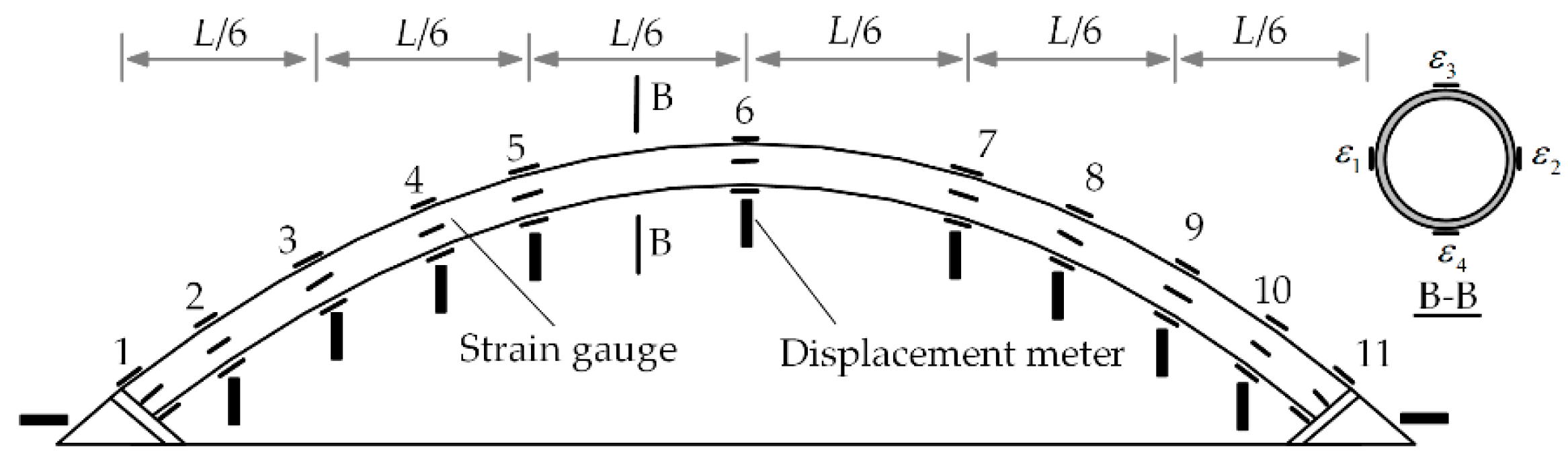
3.1. Experiment on CFST Arches under In-Plane Loads

Wu [31] conducted a experiment of nine parabolic single tube CFST arch models with different rise-span ratios and load models. Here, the arch under uniform distributed vertical loads was chosen and abbreviated to arch-A below. Arch-A was 9 m in span, 1:6 in rise-span ratio, 159 mm in diameter, and the steel tube was 4.5-mm thick. The yield stress, elastic modulus of steel and cubic compressive strength, and elastic modulus of concrete were 376.2 MPa, 204 GPa and 41.60 MPa, and 31.3 GPa, respectively. Five loading devices were set at equal intervals along the arch span, respectively, as five-point loads to simulate the process of in-plane uniformly vertical loads. As shown in Figure 2, displacement meters and strain gauges were arranged at L/12, L/6, L/4, L/3, L/2, 2L/3, 3L/4, 5L/6, and 11L/12 spans of the arch model, as well as at the arch bases, to monitor displacements and strains. Each section set four measuring points from ε₁ to ε₄. Loads were applied in steps during the loading process.

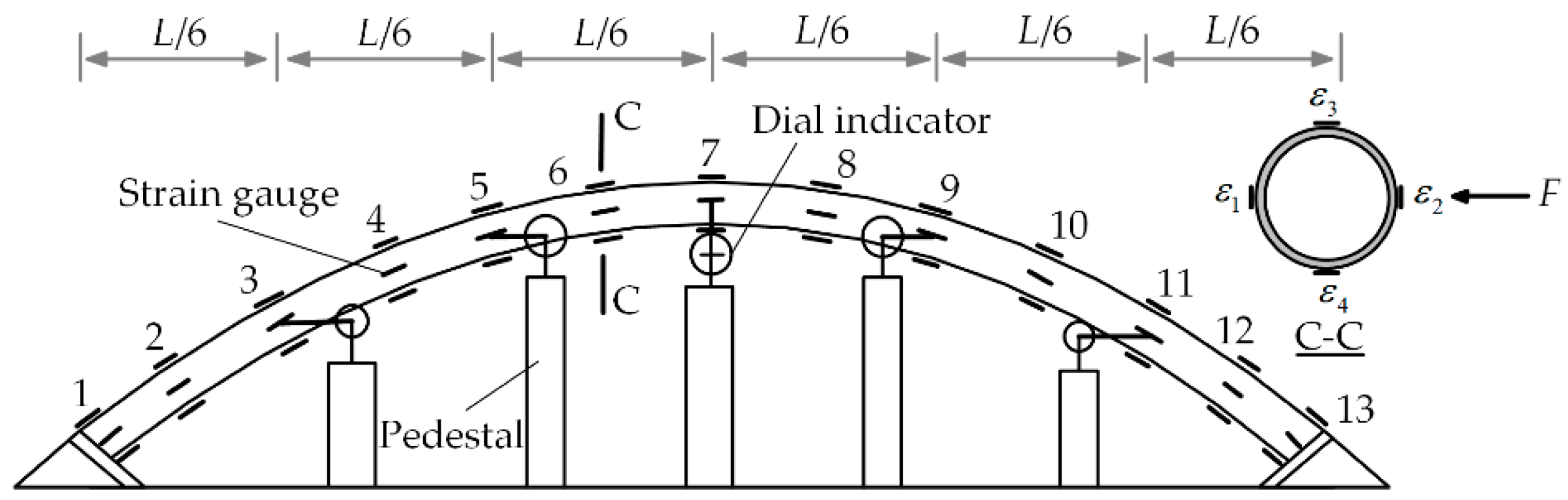
3.2. Experiment on the CFST Arch under Spatial Loads

Chen [32] experimented on a parabolic single tube CFST arch under spatial loads. To distinguish this arch model from arch-A, it is described as arch-B below. Arch-B was 7.5 m in span, 1:5 in rise-span ratio, 121 mm in diameter, and the steel tube was 4.5-mm thick. The yield stress, elastic modulus of steel and cubic compressive strength, and elastic modulus of concrete were 322 MPa, 206 GPa and 66.7 MPa, and 35.6 GPa, respectively. To simulate the process of spatial loads, five sets of loading apparatus were set at equal intervals along the arch span, respectively, to apply in-plane point loads, and a set of horizontal loading device was arranged at the arch vault to apply the out-plane point load. The measuring scheme is depicted in Figure 3. The displacement meters and strain gauges were installed at 12 equal interval sections along the span and numbered from 1–13. During the loading process, the value of horizontal load was applied to 10% of vertical loads correspondingly each time under step loading. In order to differentiate between tensile strain and compressive strain, all tensile strains are shown positive. Correspondingly, compressive strains are negative.

4. Interpolation of Experimental Data by NSF Method

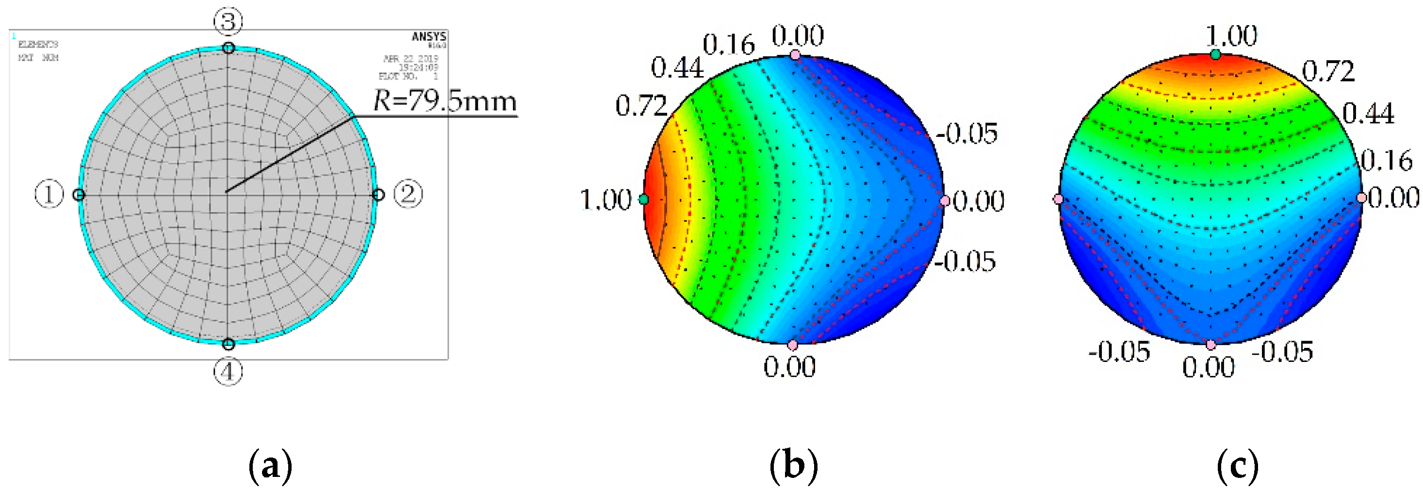
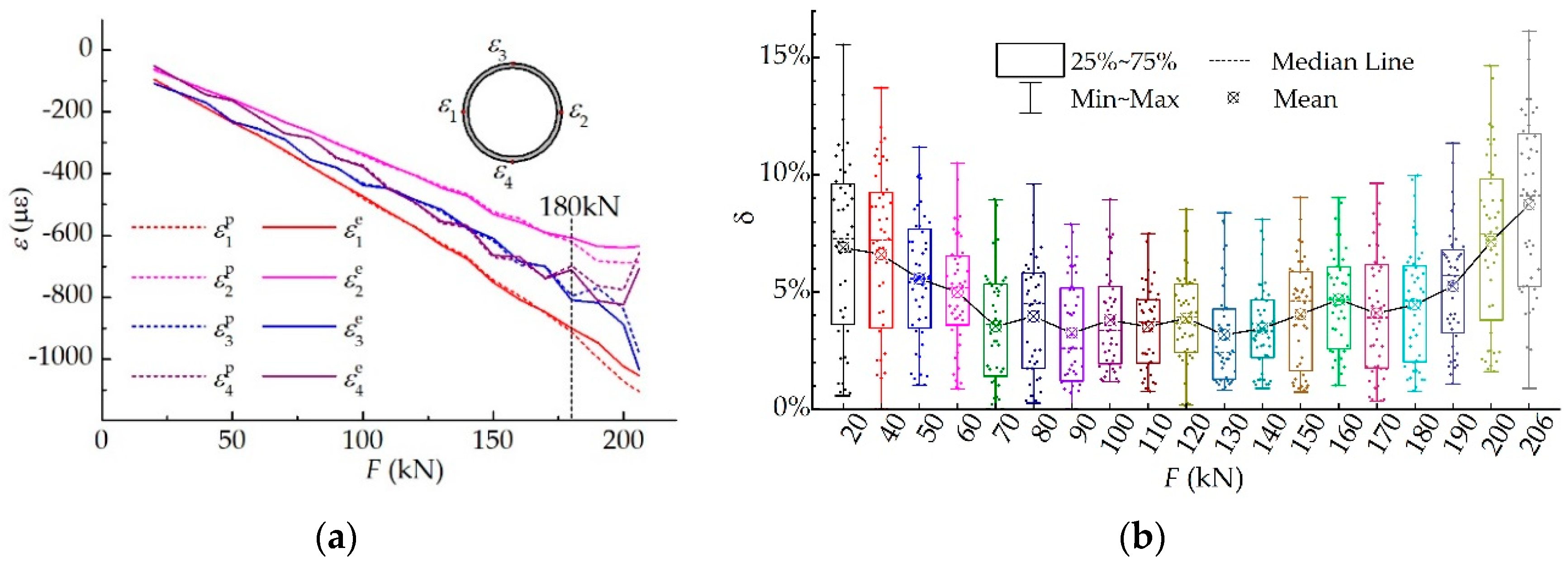
4.1. Accuracy Evaluation of NSF Method

Before applying NSF method to interpolate the strain data, the interpolation accuracy of this method should be evaluated. Here, the leave-one-out (LOO) cross-validation method was used [33]. Each of the four measured strains at the cross-section under a certain load level can be considered as a dataset of four samples. LOO-based validation was performed with four iterations, such that in each iteration, the NSF method was trained with three samples to obtain the predictive value and tested on the remaining one sample. The error δ between the predictive value ${\epsilon }_i^{\mathrm{p}}$ (i = 1, 2, 3, 4) with the real experimental sample ${\epsilon }_i^{\mathrm{e}}$ was calculated by Equation (5):

$$\delta =\left|\frac{{\epsilon }_i^{\mathrm{p}}-{\epsilon }_i^{\mathrm{e}}}{{\epsilon }_i^{\mathrm{e}}}\right|\times 100\%$$

(5)

Therefore, smaller δ equated to the better fitting degree, indicating the practicality of the method.

As an illustration, the contrast curves of strains on cross-section 4 in arch-A are given in Figure 4a. It shows that the two curves of one specific section had very high fitting degrees and even overlapped with each other before 180 kN. Thereafter, the intervals between the two curves were also very small. Figure 4b lists the validation errors of all 11 sections with different load levels. Because of the small values of strains, the little difference value between ${\epsilon }_i^{\mathrm{p}}$ and ${\epsilon }_i^{\mathrm{e}}$ would have caused great error, so the errors were relatively large in the earlier loading stage. Closer to the later part of load application, the error presented an increasing trend. This was mainly caused by random factors which started to gradually affect the structural working behavior, as well as damages in the interior of the arch, which seriously affected the interpolation accuracy of NSF method.

For all the measured strains validated by LOO, an average error of 4.79% was obtained. The error results were relatively small and greatly met the application requirement. Consequently, the NSF method can be applied with sufficient accuracy to interpolate experimental data for further investigation of the structural stressing state.

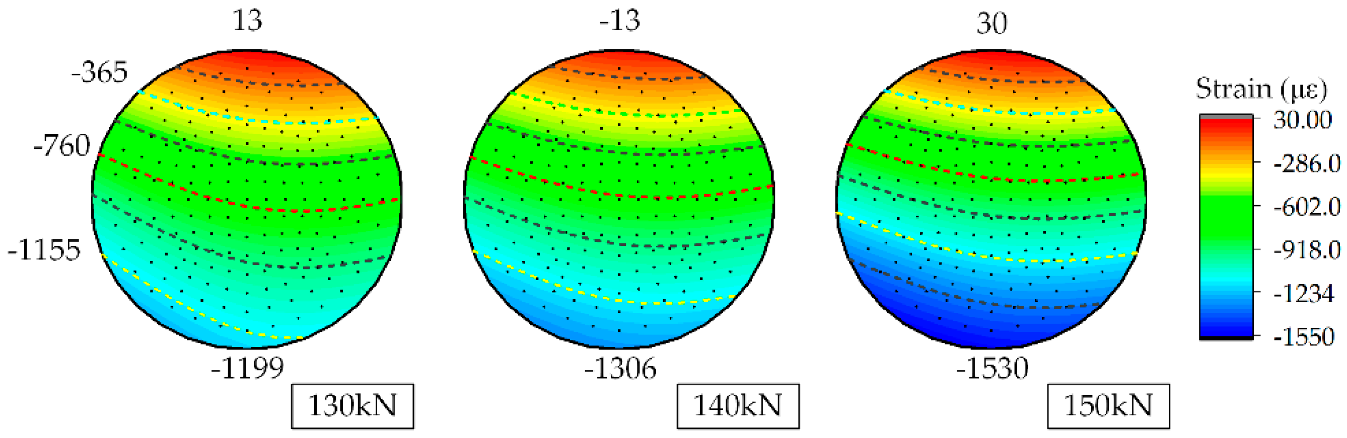
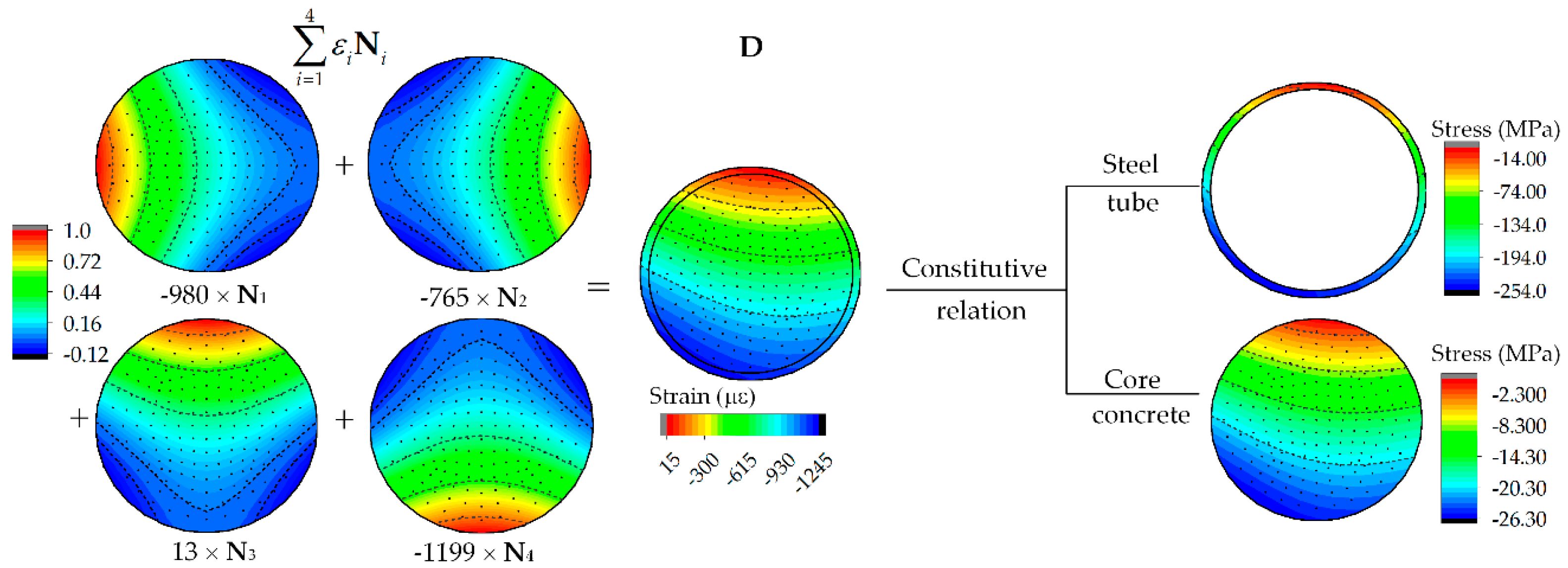
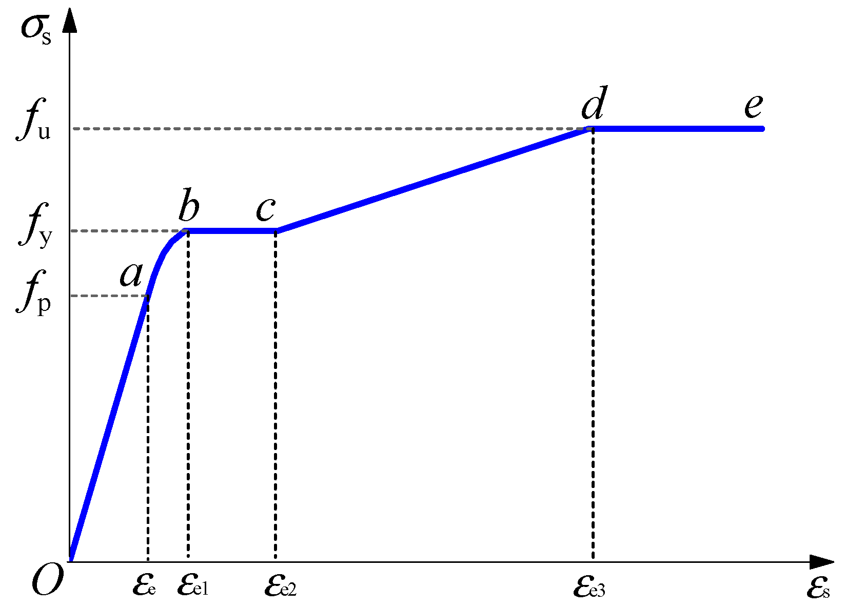
4.2. Interpolation on Strains and Stress

Before modeling the structural stressing state, the limited strains were interpolated to obtain the strain fields of each cross-section, as well as the stress fields based on the constitutive relation. Here, the software ANSYS was used to construct FE models of cross-sections, and shell element Shell 181 was chosen as the element type in consideration of its high precision. After dividing mesh, the strains of element nodes were interpolated based on the numerical shape functions N₁~N₄ with four measured strains ε₁~ε₄. Under a certain load, the interpolation strain filed D of one section was calculated by Equation (6):

$$D={\displaystyle \sum _{i=1}^4{\epsilon }_i{N}_i}$$

(6)

As shown in Figure 5, the interpolation strain field of section 11 in arch-A under 130 kN is listed as an example. The four measured strains were ε₁ = −980 με, ε₂ = −765 με, ε₃ = 13 με, and ε₄ = −1199 με, respectively. According to Equation (6), the strain field D can be obtained.

Based on strain fields interpolated by the NSF method, the corresponding stress fields could be also achieved through the constitutive relation of materials. The stress field of section 11 in arch A under 130 kN is also shown in Figure 5. When considering in the construction of constitutive relations, Equation (7), which reflects the uniaxial stress-strain relation based on numerous results [34,35], was adopted for the constitutive relationship model of core concrete in compression:

$$y=\{\begin{array}{ll}2x-x^2,& (x\le 1)\\ \frac{x}{{\beta }_0{(x-1)}^2},& (x>1)\end{array}$$

(7)

where $x=\epsilon /{\epsilon }_0$; $y=\sigma /{\sigma }_0$; ${\sigma }_0=f_c^{\prime }$; ${\epsilon }_0={\epsilon }^{\prime }+800{\xi }^2\times {10}^{-6}$; $\xi =f_y{A}_s/f_{ck}{A}_c$; ${\epsilon }_c^{\prime }=\left(1300+12.5f_c^{\prime }\right)\times {10}^{-6}$; ${\beta }_0={\left(2.36\times {10}^{-5}\right)}^{\left[0.25+{(\xi -0.5)}^7\right]}\times f_c^{\prime 0.5}\times 0.5\ge 0.12$; $f_c^{\prime }$ is the cylinder concrete compressive strength; f_y and f_ck are the yield strength of steel and the axial compressive strength of concrete; A_s and A_c are the section areas of steel and concrete; f_cu is the axial compressive strength of normative cube concrete; and f_ck = 0.67f_cu; ${\epsilon }_c^{\prime }$ is the peak strain of concrete. Equation (8) shows the tensile constitutive relation of concrete [36]:

$$y=\{\begin{array}{ll}1.2x-0.2x^6,& x<1\\ \frac{x}{{\alpha }_t{(x-1)}^{1.7}+x},& x>1\end{array}$$

(8)

where $y=\sigma /f_t$; $x=\epsilon /{\epsilon }_t$, ${\alpha }_t=0.312f_t^2$, σ is the tensile stress of concrete, f_t is the axial tensile strength of concrete and $f_t=0.26f_{cu}^{2/3}$ ε is the strain of concrete, and ε_t is the peak strain of concrete and ${\epsilon }_t=31.4f_{cu}^{0.36}\times {10}^{-6}$.

A five-stage stress-strain curve for steel tube [2] was adopted in calculation, as shown in Figure 6. At point a, there was

$${\epsilon }_{\mathrm{e}}=f_{\mathrm{p}}/E_s$$

(9)

where f_p is the proportional limit of steel, f_p = 0.8 f_y; f_y is the yield strength of steel, and E_s is the elastic modulus of steel. At point b, ε_e1 = 1.5ε_e. At point c, ε_e2 = 10ε_e1. At point d, ε_e3 = 100ε_e2. Finally, the strain/stress fields of all these cross-sections can be established for structural stressing state analysis.

Additional illustration for the method is noted. Because the experimental data itself is the reflection of structural elastic-plastic deformation, the elastoplastic behavior of the structure could be well-embodied in the interpolated strain field. Therefore, this method was used to analyze structures under the linear/non-linear state of materials. The more experimental data are measured, the more accurate interpolation results will be obtained.

5. Stressing State Analysis of CFST Arch Models

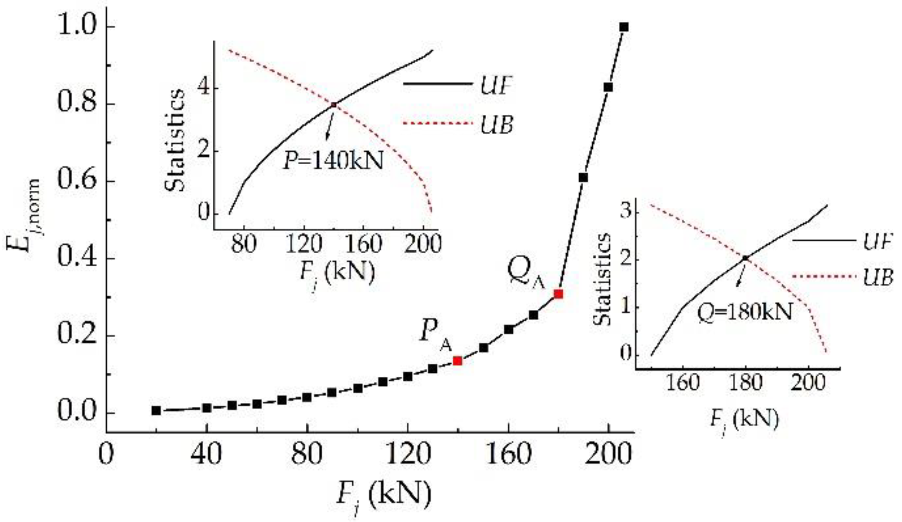
5.1. Investigation into Parameter SED for Modeling Structural Stressing State

Pursuant to the method of modeling the structural stressing state, the stressing state modes of experimental arch models were expressed by the normalized SED values to characterize their working behavior. Based on the strain/stress data interpolated by NSF method, SED values of arch-A or arch-B were calculated by Equations (3) and (4) for the expression of stressing state mode. The corresponding characteristic parameter E_j,norm under load F_j was used to plot the E-F curve in order to investigate the developing tendency and sensitivity of the arch’s stressing state mode. Using the M-K criterion, characteristic loads in the curves were detected, namely P_A (140 kN), Q_A (180 kN) for arch-A and loads P_B (66 kN), Q_B (85 kN) for arch-B, successively.

As depicted in Figure 7, the E-F curve of arch-A is plotted for example. It is shown that the curve grew rather slowly as long as the acting load remained below 140 kN (P_A), indicating that the arch model was basically in the linear-elastic working state. From 140 kN to 180 kN (loads P_A to Q_A), there was a slight growth trend of the curve, implying that the CFST arch was in the elastic-plastic working state and local plastic development existed. As the load exceeded 180 kN (Q_A), the curve thoroughly deviated from this loading path and began to undergo a fast development with rapid growth/mutation. At this stage, the arch model entered the unstable stressing state until the ultimate load (206 kN). The E-F curve of arch-B had similar developing features, so it was not discussed here.

Two common stressing state characteristics could be summarized from the above: (1) Characteristic load P is the load where the arch’s stressing state transitioned from elasticity to elastoplasticity. Although some parts in the arch model may have interred plastic states during the stages, the whole arch structure maintained a stable stressing state until characteristic load Q. In other words, the arch’s stressing state maintained quantitative change instead of qualitative change during the stages. (2) Characteristic load Q is the load where the arch’s stressing state qualitatively changed/leapt to the other state, which was different from the previous state. The arch model maintained the stable stressing state modes before load Q and then entered the gradually developing failure states until the ultimate load. It is an essential and general working behavior feature, which structures certainly present during their loading process. Hence, the load corresponding to characteristic load Q can be defined as the failure load of the structure.

The present failure at the ultimate load is a state in which structures have already been destroyed and have lost stability. To ensure sufficient safety and the normal applicability of structures, safety factors were used to multiply the ultimate load so as to be the design value for structural design. This traditional uncertain value is commonly conservative, and material is often wasted. Meanwhile, the updated failure load was revealed by the inherent mutation of the structural stressing state characteristics instead of any assumption and was in accordance with the natural law regarding the quantitative change to qualitative change of a system. That is to say, the load to structural stressing state mutation is determinate while the structural ultimate load is indeterminate. After the ultimate load was reached, the structure created a great potential safety hazard and was unsuitable for load bearing. A relatively rational safety reserve existed from the failure load to the ultimate load. Significantly, the qualitative mutation of the structural stressing state could be the common characteristic for structures and structural failure. In essence, the design load for a structure is natural law-based and definite, rather than empirical and random. Therefore, it could be a better reference to adopt the definite failure load as structural design value.

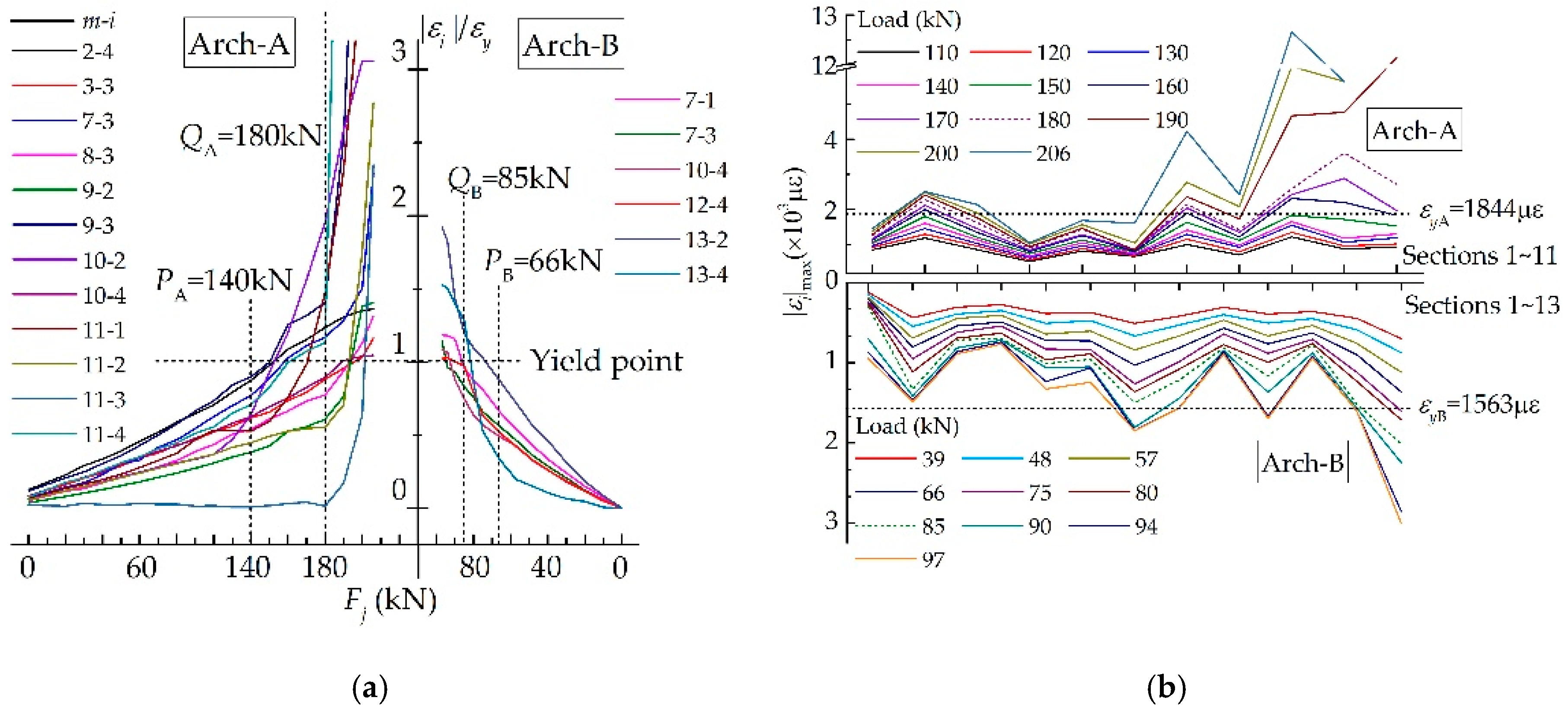
5.2. Investigation into Measured Strains of Two Arch Models

Based on the NSF method, the hidden value of structural response can be exploited by SEDs, and deep mining and analysis can be made on structural stressing state modes. However, for arches under different loading conditions, their working behaviors will have distinct performance features around the failure load (characteristic load Q). Since the measured strains of arches are the most direct reflection of their mechanical behaviors, these strains were initially selected to concretely observe their different features.

As shown in Figure 8a, the measured strain’s absolute value (|ε_i|), which reached the yield point (ε_y), was chosen. The ratio of the strain to the yield strain (|ε_i|/ε_y) was taken as a parameter to reflect the development/magnitude level of strains. The yield strains of arch-A (ε_yA) and arch-B (ε_yB) were 1844με and 1563με, respectively. It should be noted that the load F_j for arch-B here represented vertical load values, and the horizontal load was 10% of corresponding vertical loads. As seen in the figure, no yield deformations appeared before load P, and relatively small yield deformations appeared from loads P to Q. Compared with small ratios of |ε_i|/ε_y for arch-B, the strains of arch-A developed with much greater extent, especially after the failure load. Obviously, materials of arch-A were utilized to a higher degree. This is because that materials of arch-B, the failure of arch model was mainly controlled by great horizontal displacements with the action of out-plane loads, rather than material damage. To observe the distribution of strains on each cross-section, the distribution mode of the sectional maximum strain (|ε_i|_max, i = 1, 2, 3, 4) was plotted. As shown in Figure 8b, the |ε_i|_max of arch-A or arch-B maintained a slight and stable increase before the failure loads. From then on, strains of some sections showed great mutation/increment. Although the arches were loaded symmetrically, the distribution modes of |ε_i|_max were asymmetric, especially under high-level loading. The primary cause of this phenomenon was the initial geometrical imperfections of arch models.

Generally, from the perspective of experimental strain data, the arch will have a higher supporting capacity under in-plane loads than that under spatial loads and strains will have more obvious mutation characteristics around the failure load. Since the out-plane stiffness of the arch is smaller than the in-plane one, the arch model will have larger displacement under small horizontal loads, even if the materials still have subsequent bearing capacity. So, it is important to strengthen the out-plane stiffness of arch bridges, for example, by adding enough transverse supporting in practical engineering. Because the area around the arch feet is vulnerable to damage due to the impact of initial imperfection, it also should be given attention during structural design.

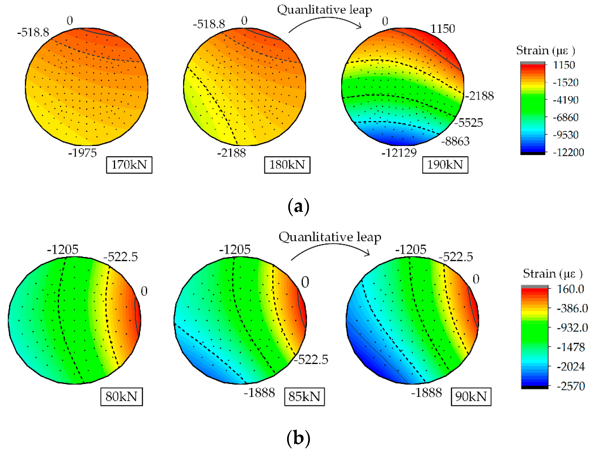
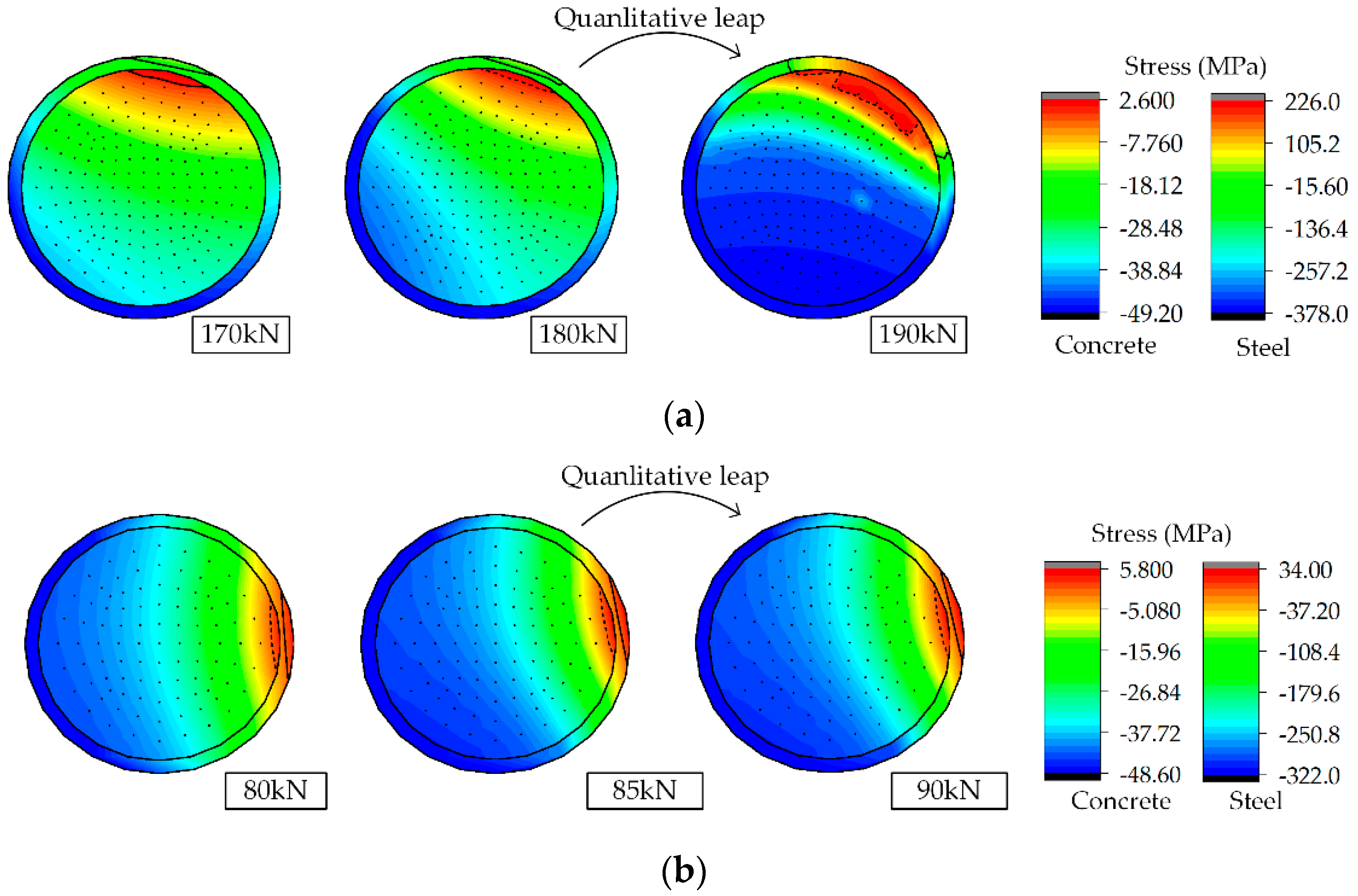
5.3. Change Characteristics Reflected by Strain/Stress Fields of Arch Models

In the light of experimental strain data, performance features of two arch models around the updated failure loads and their respective working behavior characteristics under loading can be embodied in some extent. Unfortunately, these limited data could only reflect the distribution and the development of strains of each measured point. The NSF method was applied for the strains at unmeasured points on the surface or the inside of cross-sections. Constructing strain/stress fields of cross-sections can provide an intuitive description of the structural stressing state during the loading process, as well as a clear observation of change characteristics of arch models around the failure loads. It can be seen from Figure 8 that some cross-sections of arch models had small strain values throughout the loaded process, while some others had large variation ranges and had a well-controlled effect on the arch models. Thus, the change characteristics of these key sections were the focus of attention, namely sections 7, 9–11 of arch-A, and sections 2, 7, 10, 12, and 13 of arch-B.

To observe the changes around characteristic load P, section 11 of arch-A was taken as an example. As shown in Figure 9, the strain fields were basically symmetrically distributed along the vertical. Only the densities and values of isopleth curves had slight changes before and after characteristic load P (140 kN). The strains of the whole cross-section were almost compressive, indicating that the section was mainly subjected to compression. Similar features were observed on other sections of arch-A and arch-B, and quantitative changes existed instead of qualitative changes on the shapes of isopleth and the magnitude of strain values around loads P.

To delineate the variations around characteristic point Q, section 11 of arch-A was selected. As depicted in Figure 10a, from 170 kN to 180 kN, the whole cross-section was fundamentally in the compressive state with very little tensile strains. Neither the shapes nor the values of isopleth curves had a notable distinction. From 180 kN to 190 kN, the strains of the section were still mainly compressive, even though tensile strains had obvious increments and occupied more area of the section. Especially, the compressive strain values had a dramatic growth, with a range changing from −2930~0 με at 180 kN to −12,200~0 με at 190 kN. During this stage, the oversized strain values around the lower part of the section demonstrated that the section/structure underwent an unstable stressing state with potential risk after 180 kN. Therefore, the failure load 180 kN was a watershed for the arch, implying that the arch model was considered unsuitable for resisting load from then on. Differing from arch-A, the strain values of section 13 of arch-B had a relatively small developing range due to the effect of great horizontal displacements, as shown in Figure 10b. It is seen that the area of compressive region occupied almost the whole section. With the action of spatial loads, the distribution shape of isopleth curves was asymmetric. From 80 kN to 85 kN, strains at the lower-left corner of the section had visible changes in values. When the load reached 90 kN, the changes of strains were more obvious in values and isopleth curve shapes. Potential mechanical instability caused by outer displacements limited the development of strains. Hence, the maximum compressive strain was −2570 με at 90 kN, remaining subsequent bearing capacity if the development of outer displacements can be restricted.

The stress fields of the arch models can be gained to receive a more specific stress description of steel tubes and core concrete on cross-sections. As shown in Figure 11, stress fields of typical sections are plotted. In order to clearly demonstrate stress changes of steel tube, its thickness was approximately increased without following the actual proportion of steel tube and concrete. The solid lines in steel tubes and dashed lines in core concrete signify that the stress was approaching zero. Because of the variation of section size, these lines did not overlap, but were parallel with each other. In this regard, the rationality of NSF method is shown. Considering diverse stress levels of steel and concrete, their stress color legends are listed separately in figures.

For section 11 of arch-A in Figure 11a, both concrete and steel tube underwent compressing stress before 180 kN with very small tensile stress. Obvious tensile area existed at 190 kN. The steel tube, especially, showed great tensile stress values considering that the concrete material was hardly capable of tension. The maximum tensile value, 226 MPa, was at the upper-right corner of the steel tube. Meanwhile, compressive stress born by core concrete also increased rapidly compared with the previous stable stress state. At this stage after the failure load, the mechanical behavior of both concrete and steel tube had a qualitative development. Section 13 of arch-B in Figure 11b depicts the different stressing features. Like the strain fields, the stress of the lower-left corner of the section showed obvious changes in values from 85 kN to 90 kN, while the tensile stress of the right side maintained small values.

By delineating strain/stress fields of typical sections of the two arch models, their change characteristics around failure loads can be found. Generally, owing to their different instability modes, the strain/stress fields of arch-A represent a more recognizable variation after the failure load, which can be easily distinguished from the changes of isopleth curve shapes or values in strain/stress fields.

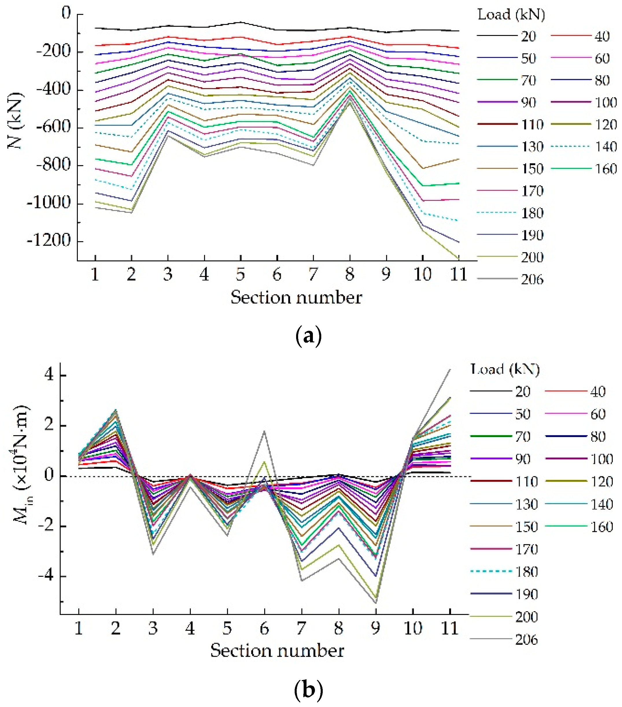
5.4. Investigation into Structural Stressing State Submodes on Internal Forces

The CFST arch models mainly underwent axial compression and bending moment. After constructing the strain/stress fields based on the NSF method, the distribution modes of sectional internal forces can also be obtained. Thus, the stressing state submodes of sectional axial forces and bending moments were built respectively to reflect their various working characteristics and evaluate their roles on arch models. Equations (10) and (11) were proposed to calculate sectional internal forces of axial force (N) and bending moment (M_y), respectively:

$$N={\displaystyle {\int }_A\sigma \mathrm{d}A}={\displaystyle \sum _A{\sigma }_i{A}_i}$$

(10)

$$M_y={\displaystyle {\int }_A\sigma y\mathrm{d}A}={\displaystyle \sum _A{\sigma }_i{y}_i{A}_i}$$

(11)

For arch-A, the out-plane bending moment was not analyzed, owing to the lateral restraint. Therefore, Figure 12 only shows the stressing state submodes of axial forces (N) and in-plane bending moments (M_in). In Figure 12a, N at section 8 was smaller than other sections. Closer to the later part of load, this phenomenon became more pronounced. Combining the great displacements and M_in at sections 7 and 9 indicates that the bending moment played a control role in the section. Before the load exceeded 140 kN, the distribution mode of N was stable with light undulation. Then, the distribution mode began to show obvious fluctuations at some sections, such as sections 2, 7, and 11. However, the mutation features around the failure load could not be clearly distinguished from the curve. In Figure 12b, it is seen that the curves were in asymmetrical distribution, especially under high-level loading. Excluding sections 7 and 9, which were mentioned previously, section 11 also had large bending moments, indicating that the area near the arch feet was subjected to heavy force. The developing trend of M_in after 180 kN changed with great increments, especially at sections 7–9, which reflected the qualitative change of stressing submodes at the failure load.

For arch-B, Figure 13 shows the stressing state submodes of axial forces (N), in-plane bending moments (M_in), and out-plane bending moments (M_out). Under normal circumstances, axial forces in arch appeared as compression, but N presented positive at section 1 while others were all negative. This may have been caused by an inaccurate measurement or geometric and material nonlinearity of the arch, and local buckling of steel tube may have also been produced. The same phenomenon occurred in the curve of M_out. Nevertheless, this did not have a large effect on the trend features of the arch’s stressing state. As shown in Figure 13a,b, the curves developed steadily with no obvious mutation changes, reflecting that the arch maintained excellent in-plane stability in all loading processes. As depicted in Figure 13c, except the M_out near the arch feet, the curves from sections 3–11 were symmetrically distributed around section 7 (the arch vault), demonstrating that the development of M_out was not sensitive to initial imperfections. Out-plane point load was applied at the arch vault, so the maximum M_out occurred at section 7. The distribution mode of M_out clearly showed great increments after 85 kN, which verifies that the updated failure load was reasonable.

From the description of stressing state submodes of internal forces, their distribution modes and developing trends were reflected. For arch-A, both the axial compression and in-plane bending moment had great effects on the structural working behavior, ultimately leading to the instability failure of the arch model. The stressing state submode curve of the in-plane bending moment clearly embodied the mutation characteristic at failure load 180 kN. For arch-B, the out-plane bending moment played the dominant role in the structural development process under spatial loads. From its distribution mode curve, it also demonstrated a leap feature at failure load 85 kN.

6. Conclusions

In this research, two single tube CFST arch models, arch-A and arch-B, with different configurations, material properties, and loading conditions, were introduced to investigate CFST arches from a unique perspective. Due to the limited strain data which could not have a clear reflection of structural working behavior, the NSF method was proposed to rationally interpolate the strains at non-sampled points. Based on the interpolation data, the strain energy density (SED) was used to model structural stressing state. With application of the M-K criterion, characteristic loads were well-distinguished and divided the stressing state into different loading stages. The revealed characteristic load Q was defined as the updated failure load, which represented the starting point of the failure process of the arch and revealed the qualitative change of structural stressing state from the stable one to the unstable one.

From the perspective of measured strains, the development degrees of strains were investigated, and it was found that the structural materials had a low exploitation and utilization under the action of out-plane loads. Based on the strain data interpolated by NSF method, the strain/stress fields of cross-sections were investigated to reflect the internal stressing features of steel tubes and core concrete, and the mutation characteristics around failure load were proved. In addition, through the stressing state submodes of internal forces, the developing tendencies of axial compression and bending moments were well-presented.

In total, the effectiveness and practicability of NSF method and the method of modeling structural stressing state were verified for revealing the stressing state characteristics of arches under different load types. The verification of these methods may provide guidance to promote engineering practice and improvement in design codes, which could considerably promote the benefits in saving material, structural safety, and structural working rationality.

References

1. Chen, B.C. Recent development and future trends of arch bridges. In Proceedings of the 7th International Conference on Arch Bridges, Trogir-Split, Croatia, 4–6 October 2013. [Google Scholar]
2. Zhong, S.T. The Concrete-Filled Steel Tubular Structures; Tsinghua University Press Publishers: Beijing, China, 2003. [Google Scholar]
3. Han, L.H. The influence of concrete compaction on the strength of concrete filled steel tubes. Adv. Struct. Eng. 2000, 3, 131–137. [Google Scholar] [CrossRef]
4. Chen, B.C. An overview of concrete and CFST arch bridges in China. In Proceedings of the 5th International Conference on Arch Bridges, Madeira, Portugal, 12–14 September 2007. [Google Scholar]
5. Zheng, J.; Wang, J. Concrete-filled steel tube arch bridges in China. Engineering 2018, 4, 143–155. [Google Scholar] [CrossRef]
6. Pi, Y.L.; Trahair, N.S. In-plane buckling and design of steel arches. J. Struct. Eng. 1999, 125, 1291–1298. [Google Scholar] [CrossRef]
7. Pi, Y.L.; Liu, C.; Bradford, M.A.; Zhang, S. In-plane strength of concrete-filled steel tubular circular arches. J. Constr. Steel. Res. 2012, 69, 77–94. [Google Scholar] [CrossRef]
8. Cheng, X.L. In-plane Stability Parabolic Concrete-Filled Steel Tubular Arches with Low Rise-Span Ratios. Master’s Thesis, Harbin Institute of Technology, Harbin, China, 2014. (In Chinese). [Google Scholar]
9. Li, Z.L.; Zhou, P.Y. Research on overall stability of concrete-filled steel tubular bowstring arch bridge. Adv. Struct. Eng. 2011, 243–249, 1988–1994. [Google Scholar] [CrossRef]
10. Yu, H.G.; Zhou, S.X.; Chen, Q.; Hu, X.L. Influence of initial stress on concrete-filled steel tubular arch bridge stability and bearing capacity. J. Changsha Univ. Sci. Technol. Nat. Sci. 2005, 2, 18–22. (In Chinese) [Google Scholar]
11. Pi, Y.L.; Trahair, N.S. Non-linear buckling and postbuckling of elastic arches. Eng. Struct. 1998, 20, 571–579. [Google Scholar] [CrossRef]
12. Geng, Y.; Wang, Y.; Ranzi, G.; Wu, X. Time-dependent analysis of long-span, concrete-filled steel tubular arch bridges. J. Bridge Eng. 2014, 19, 04013019. [Google Scholar] [CrossRef]
13. Luo, K.; Pi, Y.L.; Gao, W.; Bradford, M.A.; Hui, D. Investigation into long-term behaviour and stability of concrete-filled steel tubular arches. J. Constr. Steel Res. 2015, 104, 127–136. [Google Scholar] [CrossRef]
14. Chen, B.C.; Chen, Y.J. Experimental study on mechanic behaviors of concrete-filled steel tubular rib arch under in-plane loads. Eng. Mech. 2000, 17, 44–50. [Google Scholar] [CrossRef]
15. Liu, Y.; Wang, D.; Zhu, Y.Z. Analysis of ultimate load-bearing capacity of long-span CFST arch bridges. Appl. Mech. Mater. 2011, 90–93, 1149–1156. [Google Scholar] [CrossRef]
16. Han, X.; Zhu, B.; Liu, G.M.; Wang, J.P.; Xiang, B.S. The analysis of double-nonlinearity stability of concrete filled steel-tube arch bridge. Adv. Mater. Res. 2013, 724–725, 1709–1713. [Google Scholar] [CrossRef]
17. Deng, J.; Zhou, F.; Tan, P. Study on method for calculating spatial ultimate load of circular CFST arch. J. Build. Struct. 2014, 35, 28–35. [Google Scholar] [CrossRef]
18. Liu, C.Y.; Wang, W.Y.; Wu, X.R.; Zhang, S.M. In-plane stability of fixed concrete-filled steel tubular parabolic arches under combined bending and compression. J. Bridge Eng. 2017, 22, 04016116. [Google Scholar] [CrossRef]
19. Wang, Y.; Ye, Z.W.; Wu, Q.X. Out-of-plane buckling strength analysis for typical single tube CFST arch bridge by finite element method. In Proceedings of the 5th International Conference on Civil Engineering and Urban Planning (CEUP2016), Xi’an, China, 23–26 August 2016. [Google Scholar]
20. Wu, X.; Liu, C.; Wang, W.; Wang, Y. In-plane strength and design of fixed concrete-filled steel tubular parabolic arches. J. Bridge Eng. 2015, 20, 04015016. [Google Scholar] [CrossRef]
21. Shi, J.; Zheng, K.K.; Tan, Y.Q.; Yang, K.K.; Zhou, G.C. Response simulating interpolation methods for expanding experimental data based on numerical shape functions. Comput. Struct. 2019, 218, 1–8. [Google Scholar] [CrossRef]
22. Ayers, P.W. Information theory, the shape function, and the hirshfeld atom. Theor. Chem. Acc. 2006, 115, 370–378. [Google Scholar] [CrossRef]
23. Padhi, G.S.; Shenoi, R.A.; Moy, S.S.J.; Mccarthy, M.A. Analytic integration of kernel shape function product integrals in the boundary element method. Comput. Struct. 2001, 79, 1325–1333. [Google Scholar] [CrossRef]
24. ANSYS Help Documents; SAS IP, Inc.: Cary, NC, USA, 2015.
25. Huang, Y.; Zhang, Y.; Zhang, M.; Zhou, G. Method for predicting the failure load of masonry wall panels based on generalized strain-energy density. J. Eng. Mech. 2014, 140, 04014061. [Google Scholar] [CrossRef]
26. Shi, J.; Li, W.T.; Zheng, K.K.; Yang, K.K.; Zhou, G.C. Experimental investigation into stressing state characteristics of large-curvature continuous steel box-girder bridge model. Constr. Build. Mater. 2018, 178, 574–583. [Google Scholar] [CrossRef]
27. Kendall, M.G. Rank Correlation Methods. Br. J. Psychol. 1948, 25, 86–91. [Google Scholar] [CrossRef]
28. Mann, H.B. Nonparametric tests against trend. Econometrica 1945, 13, 245–259. [Google Scholar] [CrossRef]
29. Hirsch, R.M.; Slack, J.R.; Smith, R.A. Techniques of trend analysis for monthly water quality data. Water Resour. Res. 1982, 18, 107–121. [Google Scholar] [CrossRef]
30. Shi, J.; Yang, K.K.; Zheng, K.K.; Shen, J.Y.; Zhou, G.C.; Huang, Y.X. An investigation into working behavior characteristics of parabolic CFST arches applying structural stressing state theory. J. Civ. Eng. Manag. 2019, 25, 215–227. [Google Scholar] [CrossRef]
31. Wu, X.R. Wind Resistance during Construction and In-plane Stability after Construction of CFST Arches. Ph.D. Thesis, Harbin Institute of Technology, Harbin, China, 2015. (In Chinese). [Google Scholar]
32. Chen, B.C.; Wei, J.G.; Lin, J.Y. Experimental study on concrete filled steel tubular (single tube) arch with one rib under spatial loads. Eng. Mech. 2006, 23, 99–106. [Google Scholar] [CrossRef]
33. Geisser, S. A predictive approach to the random effect model. Biometrika 1974, 61, 101–107. [Google Scholar] [CrossRef]
34. Han, L.H.; Zheng, L.Q.; He, S.H.; Tao, Z. Tests on curved concrete filled steel tubular members subjected to axial compression. J. Constr. Steel Res. 2011, 67, 965–976. [Google Scholar] [CrossRef]
35. Han, L.H.; An, Y.F. Performance of concrete-encased CFST stub columns under axial compression. J. Constr. Steel Res. 2014, 93, 62–76. [Google Scholar] [CrossRef]
36. Gilbert, R.L.; Warner, R.F. Tension stiffening in reinforced concrete slabs. J. Struct. Div. 1978, 104, 1885–1900. [Google Scholar] [CrossRef]
Figure 1. Finite element (FE) model and numerical shape functions: (a) The FE model of the cross-section; (b) numerical shape function N1; (c) numerical shape function N3.
Applsci 09 05006 g001
Figure 2. The measuring scheme of arch-A.
Applsci 09 05006 g002
Figure 3. The measuring scheme of arch-B.
Applsci 09 05006 g003
Figure 4. The error results of strain data in arch-A: (a) Contrast curves on cross-section 4; (b) the validation errors of all sections.
Applsci 09 05006 g004
Figure 5. The strain/stress fields of section 11 in arch-A under 130 kN.
Applsci 09 05006 g005
Figure 6. The stress-strain curve of steel.
Applsci 09 05006 g006
Figure 7. The E-F curve of arch-A and characteristic loads distinguished by Mann-Kendall (M-K) criterion.
Applsci 09 05006 g007
Figure 8. The distribution curves of experimental strains: (a) |εi|/εy-Fj curve of two arch models; (b) the distribution mode curve of |εi|max. (Note: m-i denotes εi of m-th cross-section, i = 1, 2, 3, 4).
Applsci 09 05006 g008
Figure 9. Strain fields of section 11 of arch-A around characteristic point PA.
Applsci 09 05006 g009
Figure 10. Strain fields of two arch models around characteristic loads Q: (a) Section 11 of arch-A; (b) Section 13 of arch-B.
Applsci 09 05006 g010
Figure 11. Stress fields of arch models around characteristic loads Q: (a) Section 11 of arch-A; (b) Section 13 of arch-B.
Applsci 09 05006 g011
Figure 12. The stressing state submodes for internal forces of arch-A: (a) The distribution mode of N; (b) the distribution mode of Min.
Applsci 09 05006 g012
Figure 13. The stressing state submodes for internal forces of arch-B: (a) The distribution mode of N; (b) the distribution mode of Min; (c) the distribution mode of Mout.
Applsci 09 05006 g013