1. Introduction
Indoor positioning is important for location-based service, internet of things and health care [
1,
2]. Many wireless systems, such as Ultra-Wideband, Bluetooth and cellular communication systems, have been used for indoor positioning. As one of the most widely used wireless systems, the cellular communication system supports mobile phone positioning from 2G to 5G [
3]. In recent years, with the development of the location service market, the cellular communication system based positioning can be used in many new fields such as vehicle positioning [
4,
5], location-aware communications [
6] and location-based applications [
7]. The 3rd Generation Partnership Project (3GPP) also puts higher requirements on the positioning accuracy of the 5G system [
8,
9].
The TDOA-only positioning technology based on cellular communication system is relatively mature. For a long time, the cellular communication system mainly realizes the user equipment (UE) positioning through the TDOA positioning method. Long Term Evolution (LTE) system provides a TDOA estimation technology called Observed Time Difference of Arrival (OTDOA) [
10,
11]. In general, UE can only receive downlink signals from the nearest base station. Using OTDOA technology, base stations broadcast positioning reference signal (PRS) to UE. PRS has a unique mechanism named power boosting to make sure that the UE could receive PRSs from multiple sources so that multiple time-difference-of-arrival (TDOA) measurements can be obtained [
12]. UE estimates the TDOA measurements by finding the peak of correlation of the received PRS with a shifted and conjugated version of PRS [
13]. When the signal sources’ locations are known, a nonlinear equation can be constructed using sources’ locations and TDOA measurements to calculate UE’s position. There are many existing localization algorithms for the solution of the TDOA measurement equations [
14]. These algorithms can be divided into iterative methods and closed-form solutions [
15]. The iterative methods usually use the Taylor-series to linearize the nonlinear equations and use Gauss-Newton method to iterate location estimation errors. Those methods can provide accurate position estimation when the initial position is appropriate, otherwise, it cannot guarantee convergence [
16]. Closed-form solutions could avoid the convergence problem. The most used closed-form algorithm is a two-step Weighted Least squares (WLS) estimators developed by Chan and Ho [
17]. This solution can reach the Cramer-Rao lower bound (CRLB) when TDOA error is small enough. However, as the error increases, its performance would degrade. Ho also developed an improved version of the algorithm [
18]. The improved algorithm has a better performance when the variance of the TDOA measurement errors is known. The constraint equation could improve the accuracy of the closed-form algorithm. An algorithm using earth constraint can improve accuracy [
19], but this constraint is not suitable for indoor positioning. The above algorithms are often used for UE position estimation after obtaining TDOA measurements through OTDOA technology.
There are still many problems in the exiting system that make the positioning accuracy not high enough. Since the outdoor base station cannot meet the indoor signal coverage requirements, cellular communication system uses the indoor distribution system for indoor communication services [
20]. For the indoor distribution system, all TDOA-only positioning methods have the same shortcoming. In the indoor environment, deployment of communication indoor distribution system leads to a higher geometric dilution of precision (GDOP), which is not suitable for TDOA-only based positioning. The GDOP is defined as the ratio of the accuracy limitation of a position fix to the accuracy of measurements and the concept is widely used in positioning performance analysis [
21]. By calculating the GDOP, it can be found that the TDOA-only based positioning has a higher GDOP value when the receiver is not surrounded by signal sources [
21,
22]. However, in order to achieve better signal coverage and lower deployment costs, the indoor distribution antenna (ANT) of the mobile communication system is typically placed beneath the ceiling of the central area of the room. ANTs are never deployed in the indoor areas, which are near the outer wall. In those areas, UE can only receive signals from one side, resulting in a high GDOP value and low positioning accuracy.
The 5G system has the potential to solve this problem. The 5G system would also provide TDOA measurement based on OTDOA technology [
23,
24], same as the LTE system. Different from the LTE system, the 5G system could provide high-precision TOA measurement over a large bandwidth and continuous uplink and downlink signals [
25,
26,
27]. In both LTE and 5G, due to network optimization, the UE can only transmit and receive signals with the nearest signal source. This means that UE could only estimate one signal’s TOA measurement from the nearest source. TOA-only localization algorithms require at least three TOAs to perform two-dimensional position estimation. Therefore, the 5G system cannot support TOA-only based positioning. However, the 5G system could support new hybrid positioning based on multiple TDOA measurements and single TOA.
The GDOP of the TOA-only positioning is smaller than the TDOA-only positioning when the receiver is not surrounded by signal sources [
28]. Therefore, the hybrid positioning based on multiple TDOAs and single TOA will probably achieve better positioning performance than the TDOA-only positioning. TDOA-only closed-form solutions, such as Chan-Ho, are based on the assumption that measurement errors match Gauss-Markov theory. However, the random errors of TDOA and TOA measurements are not homoscedastic. It means those algorithms cannot be used for the hybrid TDOA and TOA positioning directly.
This paper aims to improve the positioning accuracy of the indoor distribution system by using multiple TDOAs and single TOA based hybrid positioning. In this paper, we establish a three-step WLS closed-form localization algorithm for heteroscedastic TDOA and TOA measurements. The first WLS provides an initial position for the last two steps. Then the algorithm uses two-step weighted least square (WLS) to estimate the final position result. We also derived the GDOP of the proposed hybrid positioning. We performed simulations in a typical indoor hall using an indoor distribution system. As shown in the simulation result, the GDOP of the hybrid positioning is lower than the GDOP of TDOA-only positioning. The simulations also show that the proposed method could approximate the CRLB when TDOA measurements errors are small enough and have the potential to achieve a better performance than two widely used closed-form TDOA-only positioning methods.
This paper is organized as follows:
Section 2 describes the system model of hybrid TDOA and TOA positioning. In
Section 3, a new closed-form localization algorithm is developed for the nonlinear and heteroscedastic hybrid TDOA and TOA positioning equations.
Section 4 analyzes the GDOP of the hybrid positioning based on multiple TDOAs and single TOA. Simulation results and analysis are presented in
Section 5. Finally, we draw our conclusions in
Section 6.
2. System Model
The ANTs are deployed at the ceiling with same height, high vertical dilution of precision makes the system cannot provide reliable vertical positioning results [
29], which is usually obtained by other sensors [
30].
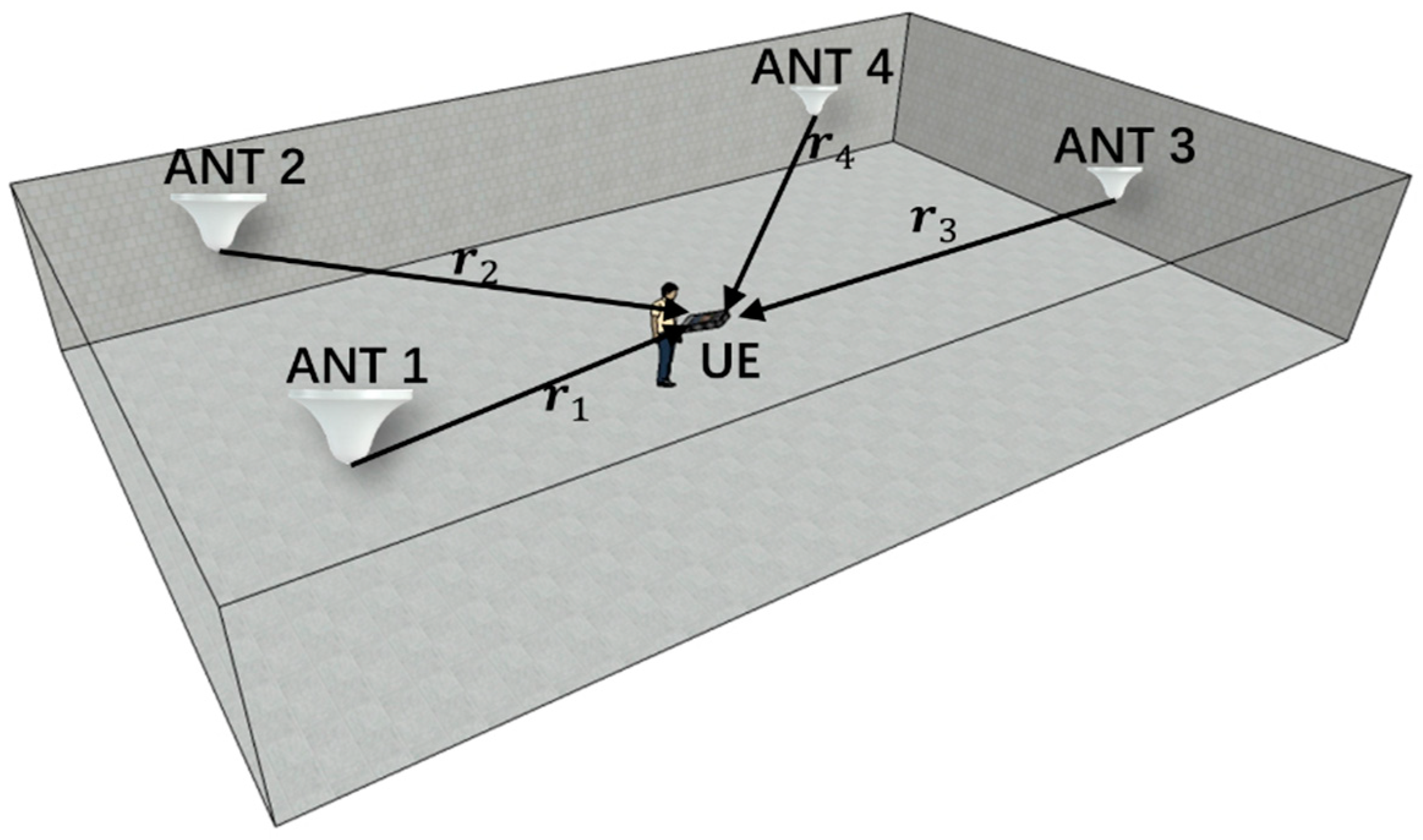
Therefore, for the system model, we assumed that ANTs are deployed at the ceiling and the height of UE is already known by other sensors, and only two-dimensional horizontal positioning is considered. The system model of the indoor distribution system based UE positioning is shown in
Figure 1. We consider a UE position estimation problem using an indoor distribution system containing
ANTs. For the system shown in
Figure 1,
is equal to 4. For each positioning process, in order to simplify mathematical representations, ANTs are sorted by the distance to the UE. The nearest ANT is numbered 1, and the farthest ANT is numbered
. UE could obtain
TDOA measurements and one TOA measurement from the nearest ANT. In
Figure 1, the nearest ANT to UE is the ANT 1 and the farthest is the ANT 4.
In the following description, the position of UE is denoted by . The system contains ANTs locating at .
The distance from ANT
to UE is expressed as
The distance difference from ANT 1 to UE and ANT
to UE is expressed as:
Considering the TDOA ranging error
, TDOA measurement from ANT 1 and ANT
is represented as:
where
is TDOA measurement and
is the speed of light,
is the distance difference calculated by TDOA measurement,
is the real distance difference and
is the ranging error caused by TDOA measurement error.
TOA measurement of ANT 1 to UE is expressed as:
where
is TOA measurement,
is the distance calculated by TOA measurement,
is the real distance from ANT 1 to UE and
is the ranging error caused by TOA measurement error.
For brevity, we denote as the TDOA ranging error and for as TDOA ranging errors between the signal from ANT and signal from ANT 1, which is denoted as in the above formula.
In a system with
ANTs, an equation system containing TDOA and TOA measurements is obtained as:
3. Three-step WLS Localization Algorithm for Hybrid Positioning
In this section, a three steps WLS localization algorithm is proposed for positioning based on TDOA and TOA measurements shown in
Section 2. The algorithm is an improvement of the two-step WLS TDOA-only localization algorithm, called the Chan-Ho algorithm, in Reference [
17]. Those two algorithms use the same linearization method, and the third step WLS of the proposed algorithm is the same as the second step WLS of the Chan-Ho algorithm.
Using the following method, a linear equation about TDOA measurement and
x, y coordination could be obtained. Moving the
from the right side of Equation (2) to the left side and then squaring both sides, we obtain:
Expanding (6) we obtain:
where:
Different to the Chan-Ho algorithm, the proposed algorithm needs to consider the TOA measurement and uses a new solution as follows. Using Equation (8), write Equation (5) in matrix form as:
where:
The vector
is the error between
and
. It can be obtained by:
In accordance with Equations (3) and (4), the items in vector
can be written as the following expressions:
where the assumption
has been used. To minimize
, the hybrid positioning problem is cast as the following quadratic optimization
Ranging errors of TDOAs can be assumed as an independent, identical and zero-mean Gaussian distribution [
31]. The ranging error of TOA can also be assumed to be a zero-mean Gaussian distribution [
32]. Because TDOA and TOA measurements are estimated using different techniques, TOA and TDOA ranging errors can be assumed to be independent and have different variances. The parameter
is used to represent the ratio of TOA ranging error’s standard deviation to TDOA ranging error’s standard deviation. The ranging errors have the following statistical properties:
The errors in
do not meet the Gauss-Markov assumption, ordinary least squares estimator is not the best linear unbiased estimator (BLUE) for this optimization problem. WLS could make it BLUE when each weight is equal to the reciprocal of the variance of the error [
33]. The WLS solution of
that minimizes
is:
where
is the weighting matrix which could be given by the covariance matrix of
.
The covariance matrix of
is:
where
is the inverse of the covariance matrix of
,
is obtained by prior probability statistics of the ranging errors after the system deployed.
Scaling of
does not affect the result of WLS [
17]. Therefore, the weighting matrix
can be written as:
However, the distances from ANTs and UE is unknown, to approximated the matrix , an initial guess of UE position is need to be obtained in first-step WLS.
3.1. First-Step WLS
To calculate the initial position, we assume that the distances from ANTs to UE are equal to the ratio
k. Rewriting the weighting matrix
as
:
We could obtain
using Equation (16) as
It is an ordinary least squares. When the UE positions are different, the deviation of the weighting matrix and the initial positioning error would change. The second-step WLS could mitigate this error and can be repeated again to give an even better estimate.
3.2. Second-Step WLS
After achieving the initial position
, the distance
from ANT
to
can be calculated. Inserting
and
into Equation (18), the weighting matrix
could be rewritten as
:
Inserting matrix into Equation (16) in the same way as Equation (20), the solution can be obtained.
3.3. Third-Step WLS
The former two steps assume no relationship between the UE location
and
, but in fact they are related. Chan-Ho algorithm has the same problem in its first stage minimization and use a WLS to refine the result [
17]. In the third-step WLS of this proposed algorithm, the same method as the Chan-Ho algorithm is used to refine the result of former two steps.
The former two steps’ results location
and distance
have a relationship shown in Equation (22). Therefore, the third-step WLS is to minimize the sum of the squared errors
in:
Equation (22) could be rewritten in matrix form as:
where:
Because elements in vector
have different variances, we need to use WLS to estimate the solution
as:
where weighting matrix
could be obtained by calculating the covariance matrix of
. Assuming that the error of the solution
in second-step WLS are
, vector
could be obtained as:
where the second-order error terms are ignored.
The matrix
could be approximated by using
as
and
could be approximated as
[
17].
Therefore, result
could be calculated by
The is the square of the difference between final positioning result and ANT 1 on the x-axis and the y-axis. As with the Chan-Ho algorithm, is given by the square root of and ANT 1’s location .
4. GDOP of the Proposed Hybrid Positioning
GDOP is the ratio of the accuracy limitation of a position fix to the accuracy of measurements [
21]. A positioning system has a small GDOP means that the positioning is accurate. In order to compare with GDOP of TDOA-only positioning, the GDOP of the proposed hybrid positioning is defined as the ratio of the positioning accuracy to the TDOA ranging accuracy.
In this section, the GDOP of the hybrid positioning based on multiple TDOAs and single TOA is derived.
To achieve the GDOP of the hybrid TDOA and TOA positioning of the system described in
Section 2, the difference between TDOA measurements and real distances difference when UE is at the location
can be expressed as:
Difference between TOA measurements and real distances when UE is at the location
is expressed as
Using a first order Taylor series to approximate Equations (6) and (7), the approximation of
at location
can be obtained as
When there are no ranging errors, (9) can be obtained from (8).
where
is UE’s real location.
To simplify the mathematical derivations, we use
to represent the TOA ranging error. Moreover,
,
, is used to represent TDOA ranging errors between the signal from ANT
and signal from ANT 0, which is represented as
in
Section 2. As the measurements have ranging errors
, Equation (33) can be obtained from (31):
where
is the position estimation result.
Let position estimation error vector
,
,
. Subtracting Equation (33) from Equation (32), the equation of
and
can be obtained as:
For TOA ranging error
, it is easy to obtain partial differential equations:
For TDOA ranging error
, partial differential equations is:
Therefore, Equation (34) can be formulated as the following matrix form:
where:
Different from the GDOP calculation process in [
21], TOA and TDOA measurements ranging errors have different variances. Therefore, in order to make an unbiased and efficient estimator, the vector
cannot be calculated based on the ordinary least square (OLS) but weighted least square (WLS) as the following expression:
where the weighting matrix W could be given by covariance matrix of error vector
.
Therefore, we could get a covariance matrix of error vector
E as:
Therefore, the weighting matrix
W in Equation (39) could be given as
Expressing matrix
as
From Equation (39),
can be calculated by:
where
The mean of
could be calculated by:
The variance of
could be calculated by:
It is easy to obtain the mean and variance of
using the above equations:
where:
GDOP was been definite as the ratio of the accuracy of a position fix to the accuracy of measurements [
34]. In order to directly compare the GDOP of the proposed hybrid positioning and the GDOP of TDOA-only positioning, we redefine the GDOP of the hybrid positioning using multiple TDOAs and single TOA as the ratio of the accuracy of a position fix to the accuracy of TDOA measurements. The GDOP could be calculated as:
5. Simulation Results and Analysis
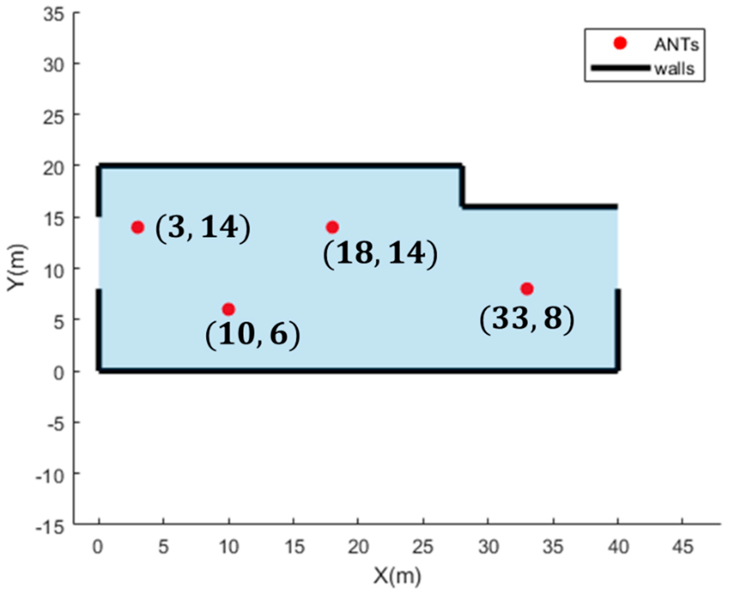
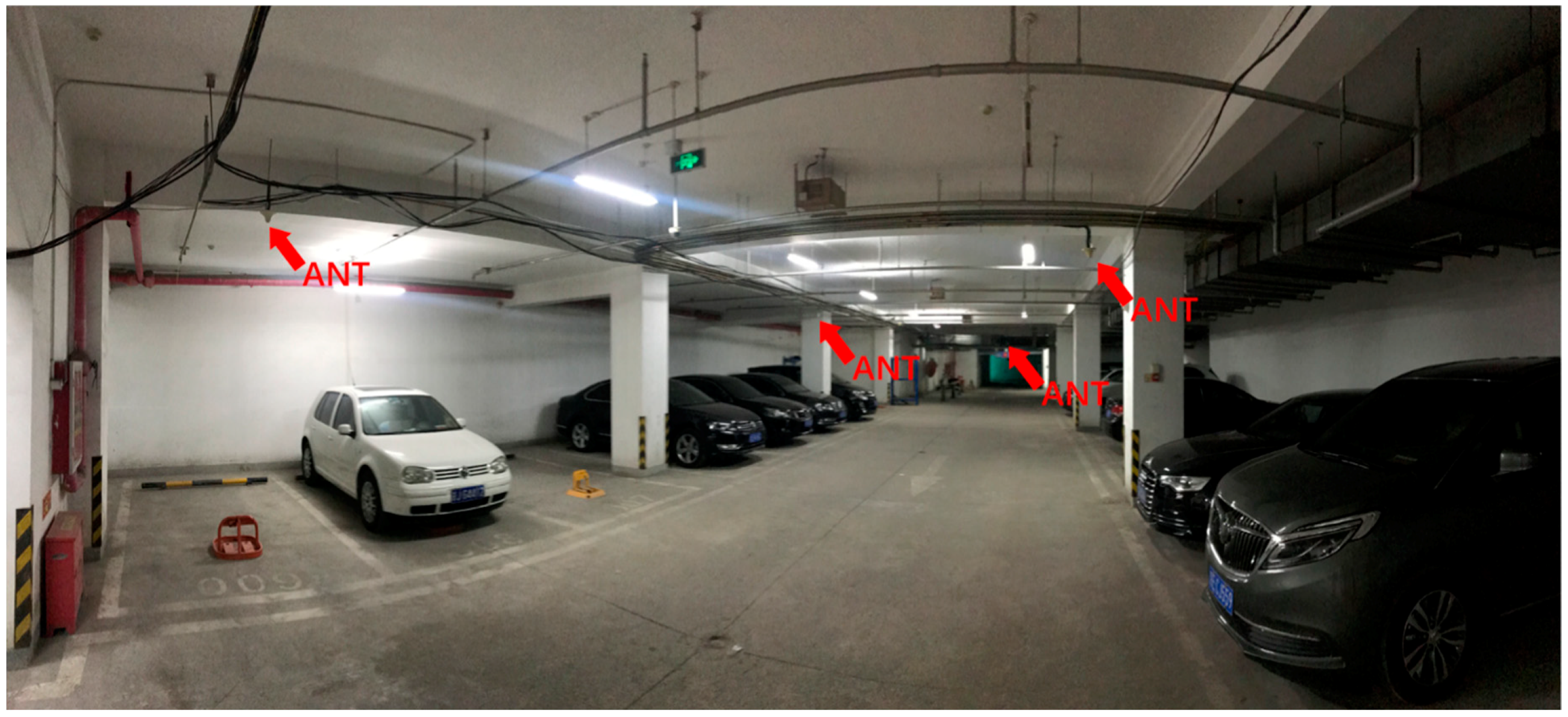
To analyze the GDOP of multiple TDOAs and single TOA based hybrid positioning and the positioning accuracy of the proposed closed-form localization algorithm, we have built a simulation scenario according to the real scene of the zone 1, underground parking lot, Beijing University of Posts and Telecommunications. The real scene is shown in
Figure 2 and the top view of the developed simulation scenario is shown in
Figure 3.
In
Figure 3, a Cartesian coordinate system is constructed in meters. The ANTs of the indoor distribution system are referred to the real antennas’ location in the underground parking lot.
In the following parts of this section, we compared the GDOP of the proposed hybrid positioning and the GDOP of TDOA-only positioning. Then, we analyzed the positioning accuracy of the proposed localization algorithm.
5.1. Analysis and Comparison of GDOP
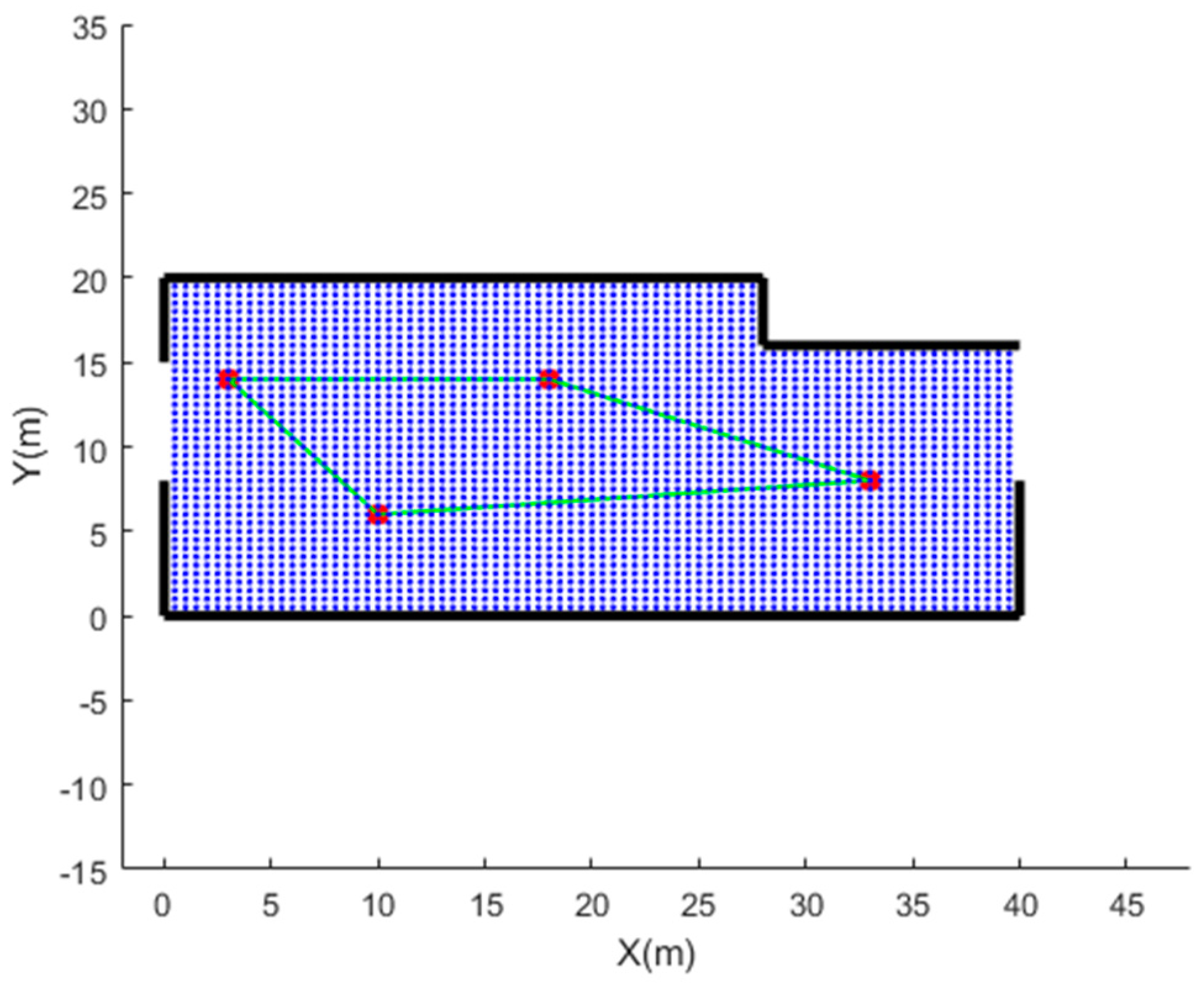
To compare the GDOP of the TDOA-only positioning and the GDOP of the hybrid positioning using multiple TDOAs and single TOA in the same indoor scenario. 2889 points is selected every 0.5 m, as shown in
Figure 4. We divide the selected points into two groups. One group contains the points within the quadrilateral surrounded by connections between ANTs, which is the green quadrilateral in
Figure 4. The other group contains the points outside the quadrilateral. 2292 points are outside the green quadrilateral and 597 points are inside the green quadrilateral.
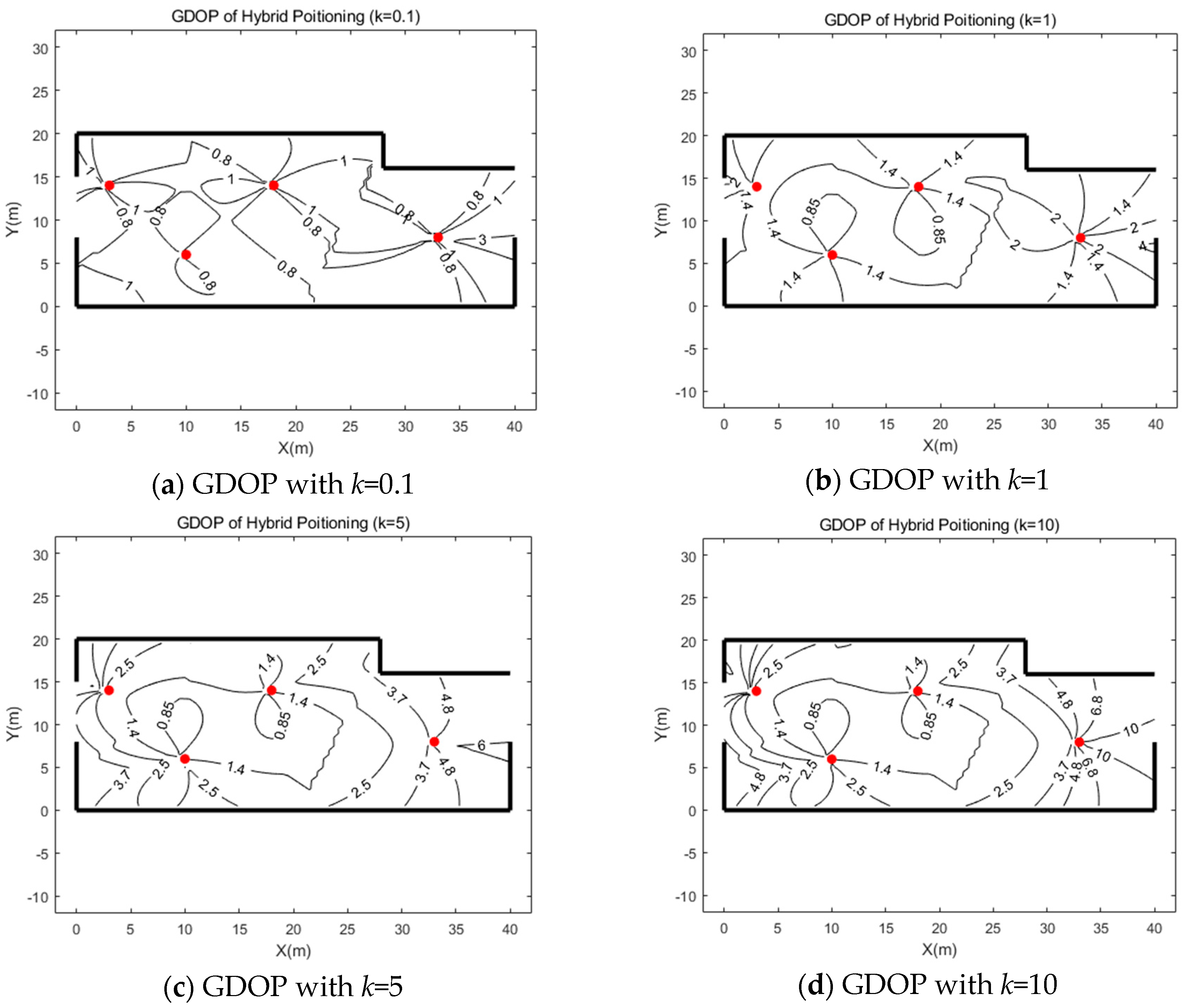
The GDOPs of the hybrid positioning method based on three TDOAs and one TOA with different ratio
values are calculated at each points. The
is the ratio of TOA ranging error standard deviation to TDOA ranging error standard deviation definite in
Section 4. We use four different
k values and the result is shown in
Figure 5.
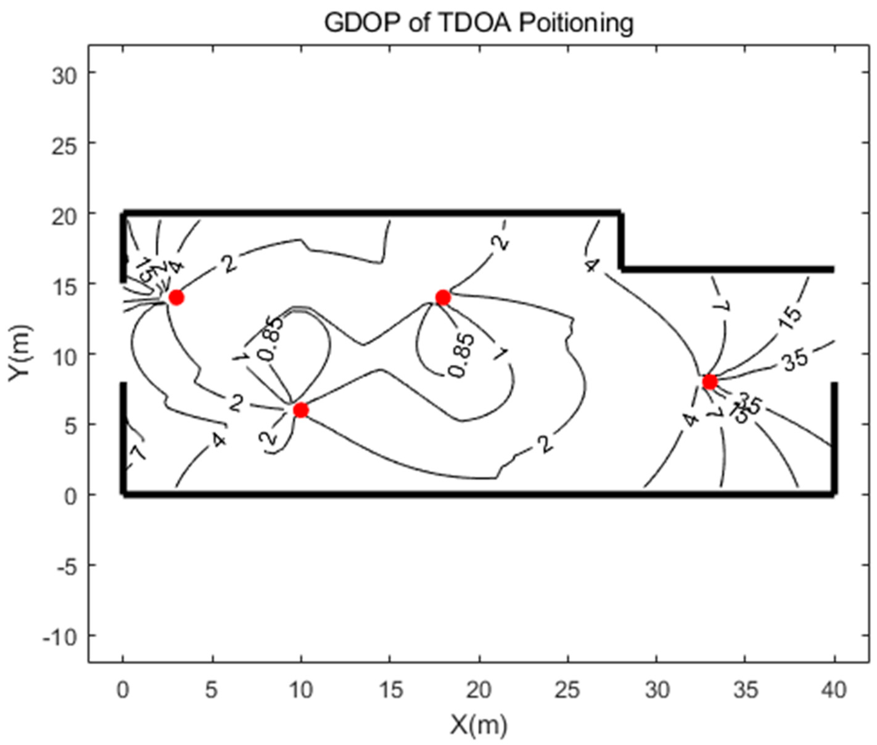
Figure 6 shows the GDOP of TDOA-only positioning in the same scenario. The TDOA-only positioning is based on three TDOA measurements which are the same as the proposed hybrid positioning method used above. The GDOP calculation method for TDOA-only positioning is similar to that GDOP calculation method for hybrid positioning described in
Section 5 but does not contain the TOA measurement terms. The calculation method is the same as the method described in the definition of GDOP [
21].
It can be easily seen from the comparison between
Figure 5 and
Figure 6 that the GDOP of the TDOA-only positioning is not much different from the hybrid positioning in the center region (the quadrilateral area surrounded by the four ANTs). In other regions, the GDOP of hybrid positioning is significantly smaller than the TDOA-only positioning. However, the area of the center region only accounts for one-fifth of the total area. Assuming that the distribution of UEs is uniform, in most cases, using the hybrid positioning method will increase the positioning accuracy limitation.
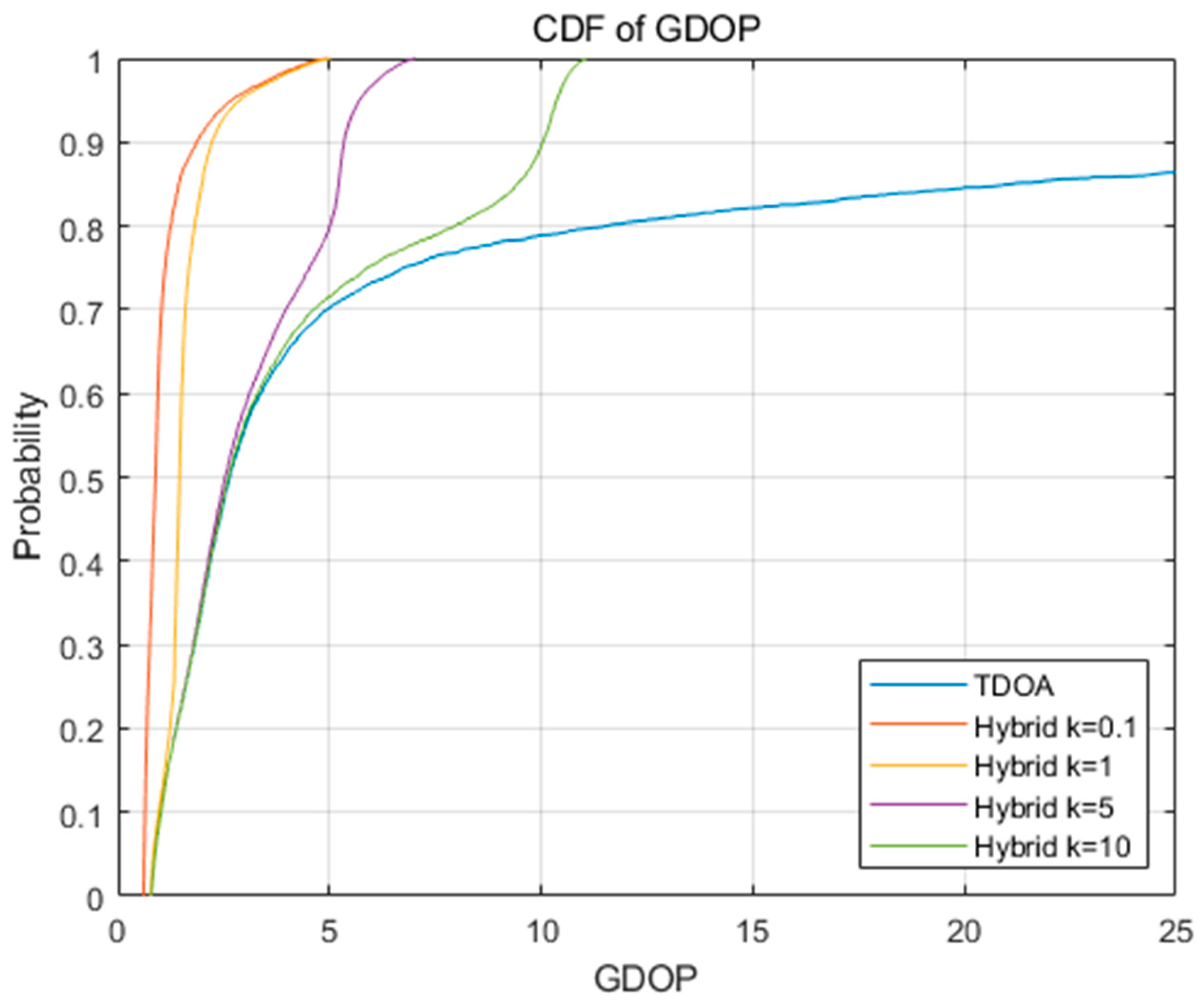
The cumulative distribution functions (CDFs) of GDOPs is obtained and shown in
Figure 7.
From
Figure 7, it is obvious that the GDOP values of the proposed hybrid positioning are significantly lower than the TDOA-only positioning. It can be seen in (16) that the greater the ratio
k is, the smaller the weight of the TOA ranging error item in the weighting matrix (18) is, and the closer the GDOP calculated is to the GDOP of TDOA-only positioning. The result shows that it is possible to effectively improve the positioning performance by adding a TOA measurement.
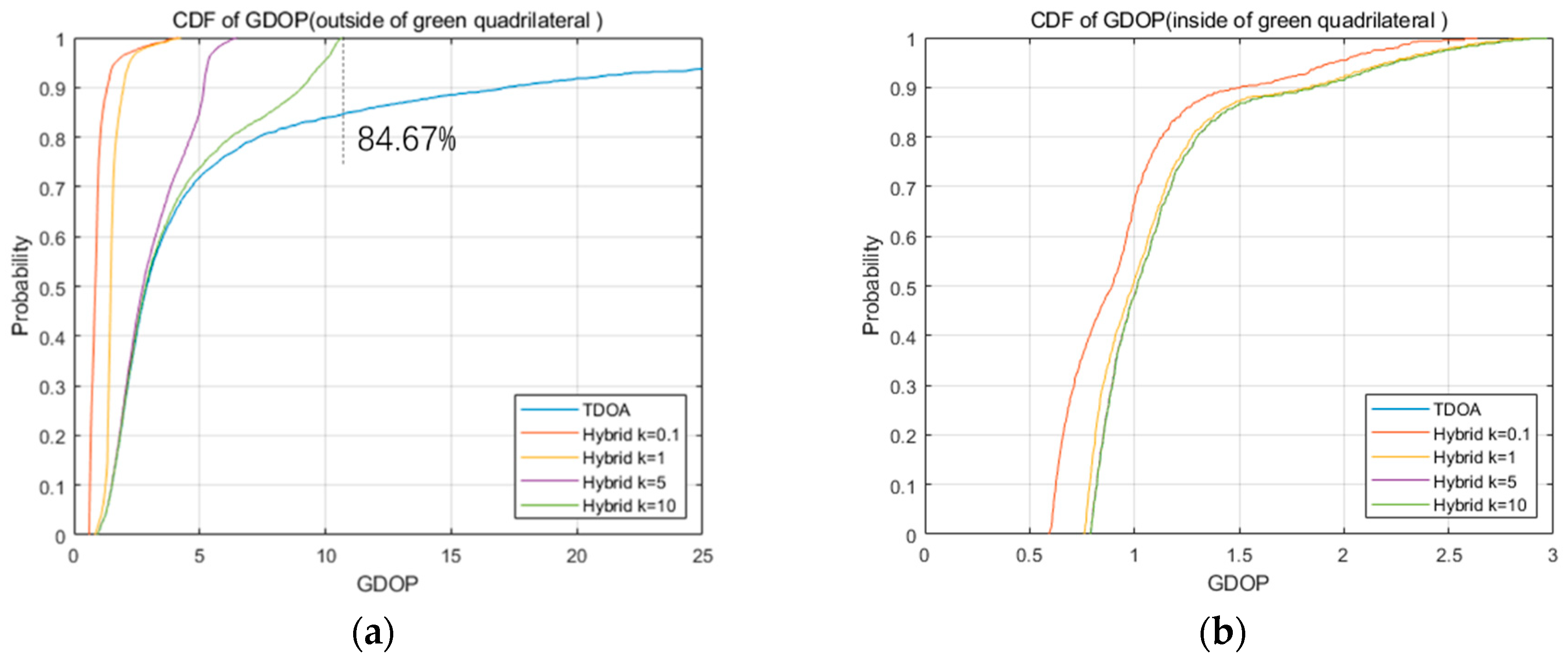
To compare the GDOPs of the two kinds of positioning in the two different regions as shown in
Figure 4, we separately counted the GDOPs of two kinds of positioning at points in the two groups. The CDFs of the GDOPs are shown in
Figure 8.
As shown in
Figure 8a, at the points outside the green quadrilateral, GDOPs of the proposed hybrid positioning are significantly lower than the TDOA-only positioning. Even when the standard deviation of TOA ranging error is 10 times the TDOA ranging error, the 24.85% points still have a higher GDOP of the TDOA-only positioning than the highest GDOP of the proposed hybrid positioning. However, as shown in
Figure 8b, at the points inside the green quadrilateral, GDOPs of the proposed hybrid positioning are not much different than GDOP of the TDOA-only positioning. Even when the ratio
k is equal to 0.1, the minimum GDOP of the proposed hybrid positioning is 0.59. And the minimum GDOP of the TDOA-only positioning is just 0.79, which is only 0.20 higher. When the ratio
k is equal to 1, 5 and 10, the GDOPs of the proposed hybrid positioning are approximate to the GDOP of the TDOA-only positioning.
Analysis result shows that adding a TOA measurement to the TDOA measurements to achieve hybrid positioning have potential to greatly improve the positioning ability of the system in the edge area of the network. At the same time, in the core area of network coverage, although hybrid positioning has only a limited improvement in positioning ability, it is also superior to the TDOA-only positioning.
5.2. Analysis and Comparison of the Proposed Localization Algorithm
CRLB is the theoretical lower bound on the variance of unbiased estimator [
35]. In order to analyze the performance of the proposed three-step WLS closed-form localization algorithm, we compare the algorithm with CRLB of the proposed hybrid positioning, CRLB of TDOA-only positioning and two widely used TDOA-only closed-form localization algorithms, Chan-Ho [
17] and BiasRed [
18]. CRLB is the trace of the inverse matrix of the Fisher information matrix [
19].
where matrix
and
are defined in
Section 3.1,
is a
matrix as
5.2.1. Simulations at Selected Point
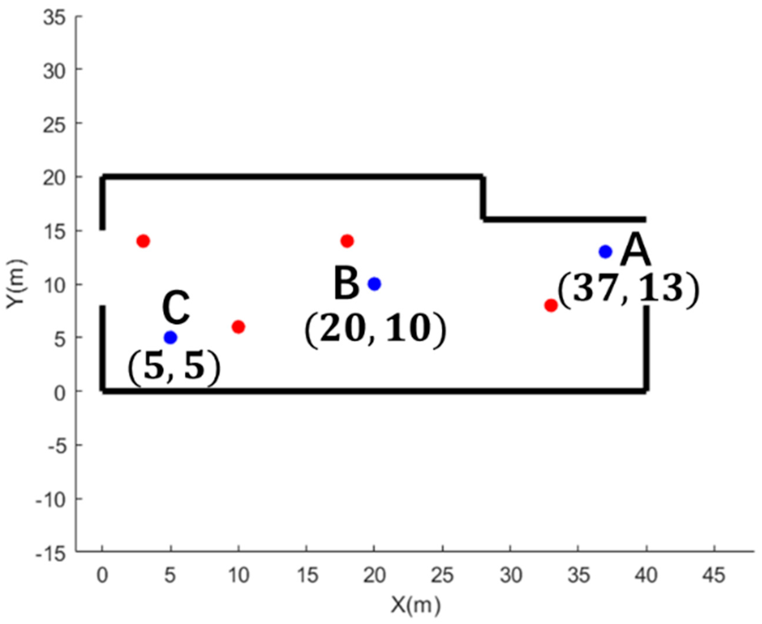
According to the GDOP analysis in
Section 5.1, we selected three test points at the right edge, the center, and the left edge of the scenario. Scenario shown in
Figure 3 is used, and three test points are selected for the simulation, which is shown in
Figure 9.
The simulation was performed 10,000 times at each test point. TDOA and TOA ranging errors were the zero-mean Gaussian distribution but with different standard deviations.
5G system could provide a TOA ranging accuracy with standard deviation
or
[
25] and provide a TDOA ranging accuracy with a best
[
13].
In each simulation, we calculated the Mean Square Error (MSE) of the positioning errors for each test points as
where
and
are the coordinate of the test point,
and
are the positioning result of the ith calculation.
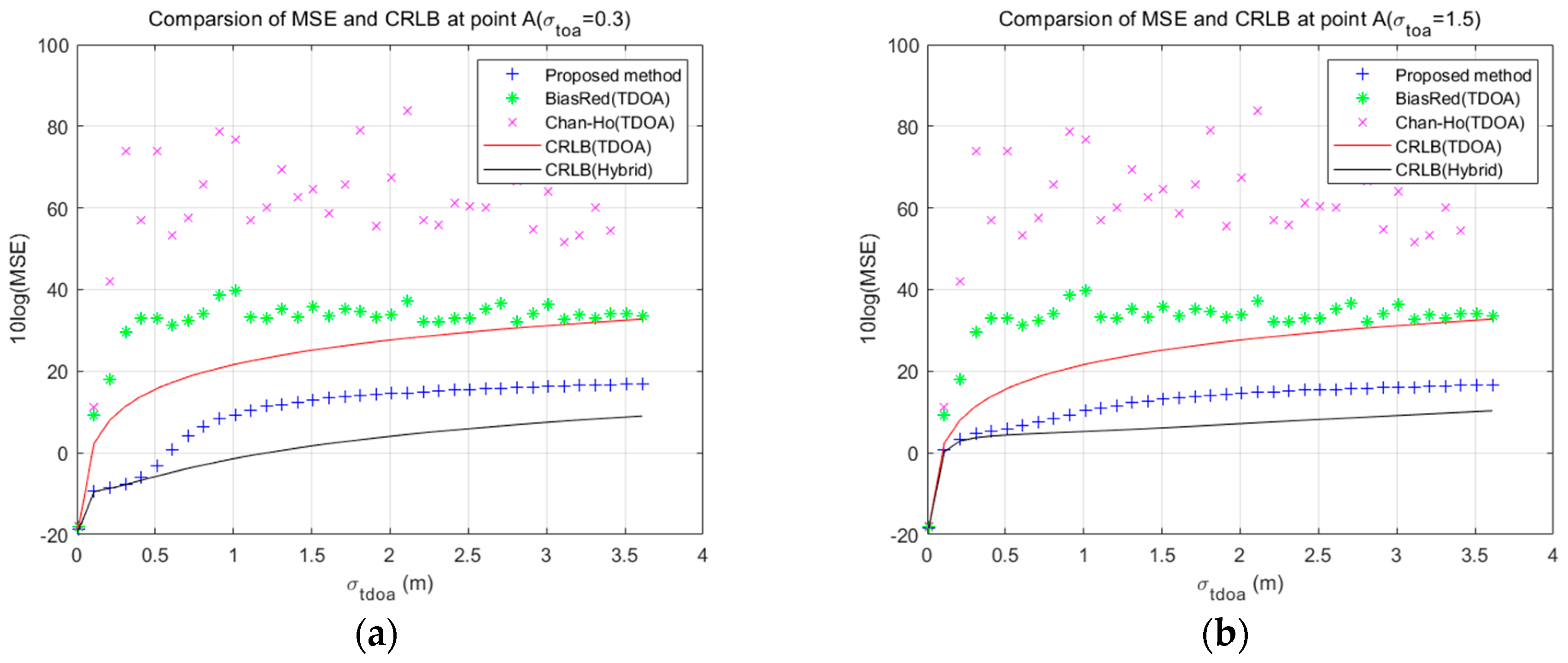
Figure 10 shows the MSE of the positioning results and the calculated CRLBs at test point A. The result shows that the positioning using multiple TDOAs and single TOA has a lower CRLB than TDOA-only positioning. Regardless of whether
or
m, the MSE of proposed algorithm approaches CRLB when TDOA ranging error is small. When the TDOA ranging error is high, the positioning error of the proposed localization algorithm is higher than the CRLB but is still significantly lower than the other two TDOA-only closed-form algorithms. For the proposed algorithm, the positioning results with
m are slightly better than the positioning results with
m when the standard deviation of TDOA ranging error is around 0.5 m.
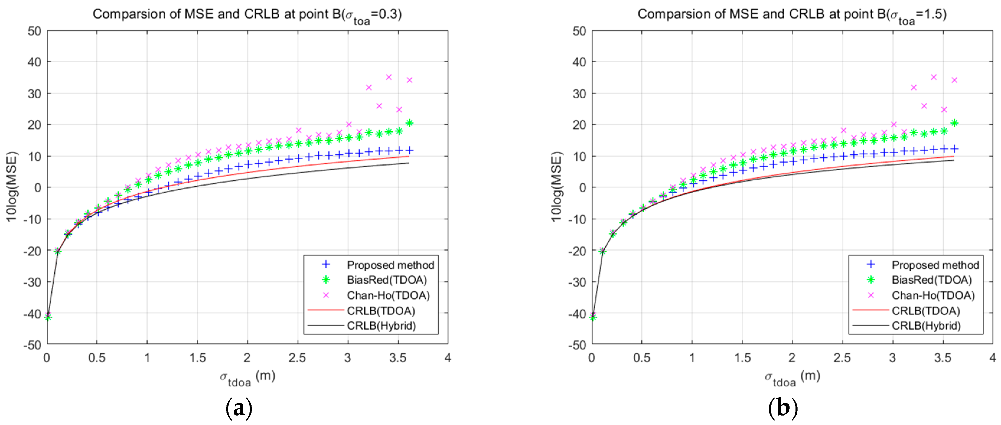
Figure 11 shows the MSE of positioning results and CRLBs at test point B. The result shows that the CRLB of the proposed hybrid positioning is close to the CRLB of TDOA-only positioning at test point B. Regardless of whether
or
m, the MSE of proposed algorithm approaches CRLB when TDOA ranging error is small. Even when the TDOA ranging error is higher, the positioning error of the proposed algorithm is only slightly higher than the CRLB. For the proposed algorithm, the positioning results with
m are slightly better than the positioning results with
m. However, regardless of the different performance caused by TOA ranging error, the positioning error of the proposed algorithm is lower than the other two TDOA-only positioning methods.
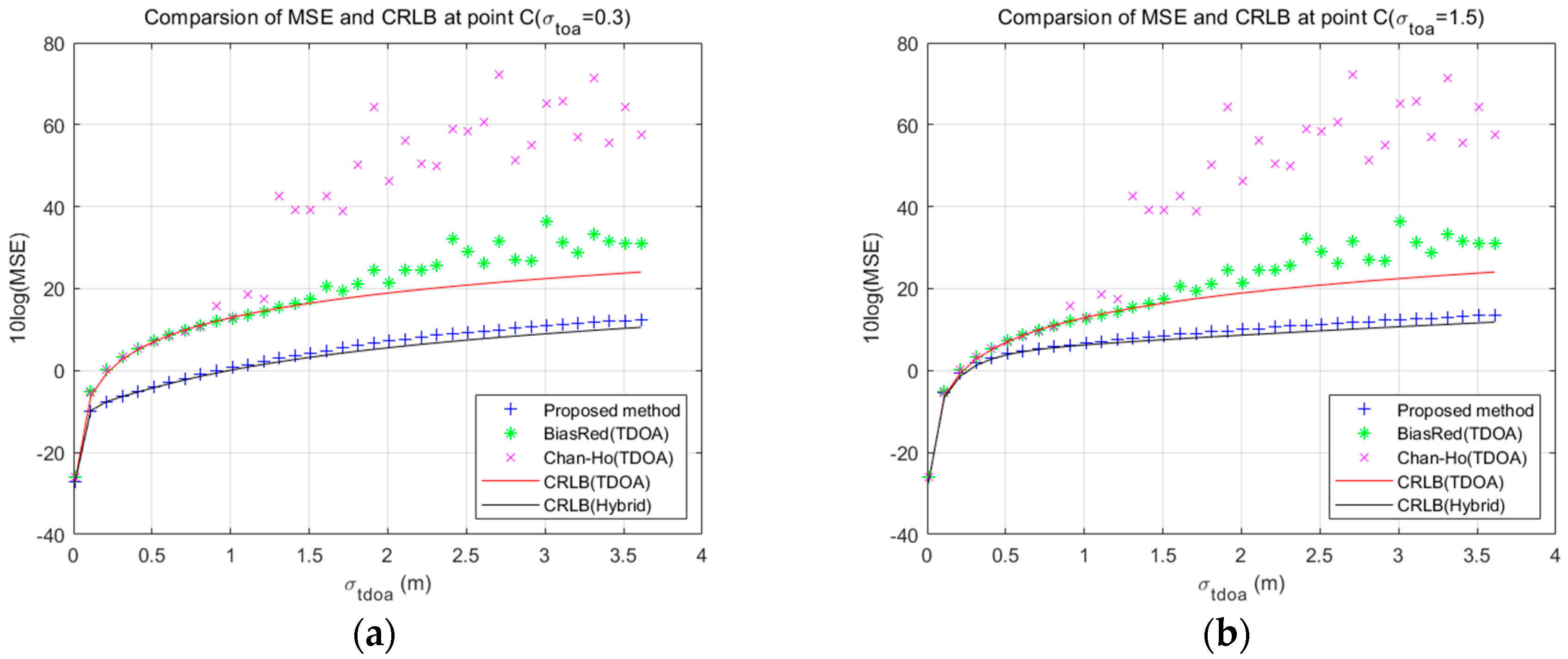
Figure 12 shows the MSE of positioning results and CRLBs at test point C. The result shows that the proposed hybrid positioning has a lower CRLB than TDOA-only positioning at test point C. Regardless of whether
or
m, the MSE of proposed algorithm approaches CRLB when TDOA ranging error is small. Even when the TDOA ranging error is higher, the positioning error of the proposed algorithm is very slightly higher than the CRLB. For the different results in (a) and (b), the proposed algorithm is more accurate while
m than
m, when the standard deviation of TDOA ranging error is around 0.5 m. However, regardless of the different performance caused by TOA ranging error, the positioning error of the proposed algorithm is significantly lower than the other two TDOA-only positioning methods.
It can be seen from those three figures that the positioning error of Chan-Ho and BiasRed would increases irregularly with the increase of the error after the error becomes larger. This may be caused by the error of the weighting matrix of those algorithms. Those two algorithms use WLS in the calculation process and ignore some items about TDOA ranging errors to build the weighting matrix. When TDOA ranging errors are small, the weighting matrix is closed to be right. However, when the ranging errors are large, the error of the weighting matrix would increase. The positioning error, caused by weighted matrix, is irregular. The proposed algorithm also has this problem, but the item about TOA measurement in weighting matrix is not related with ranging error. This may inhibit the irregularity of the positioning error when TOA ranging error is low. The positioning error of the proposed algorithm would also increases irregularly when TOA ranging error is high.
5.2.2. Simulation Results in Different Regions
To compare the positioning accuracy of the three localization algorithms in different regions, the two groups of selected points in
Figure 4 were used for simulation.
The positioning simulation is performed 10,000 times at each test point. For each test point group, the MSE of the positioning errors for each group test points was calculated and denoted as
where
and
are coordination of the
pth test point in the group,
and
are the positioning result of the
ith calculation at the
pth test point. The
of the two groups’ positioning results is counted separately. The MSEs and CRLBs of positioning results with different TDOA ranging error of the two groups are shown in
Figure 13 and
Figure 14.
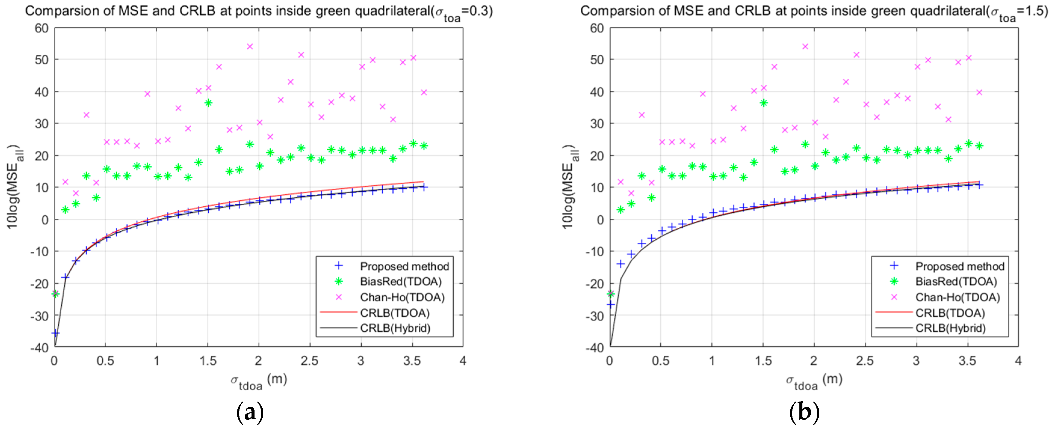
Figure 13 shows the
of the positioning results and CRLBs at test points inside the green square. The result shows that the CRLB of the proposed hybrid positioning is close to the CRLB of TDOA-only positioning. When
m, the
of proposed algorithm approach CRLB. When
m, the accuracy of the proposed algorithm is slightly higher than the CRLB while the standard deviation of TDOA ranging error is relatively small but has not yet approached zero. For the proposed algorithm with different TOA ranging error, the positioning results with
m are very slightly better than the positioning results with
m. However, regardless of the different performance caused by the TOA ranging error, the positioning error of the proposed hybrid positioning method is significantly lower than the other two TDOA-only positioning methods.
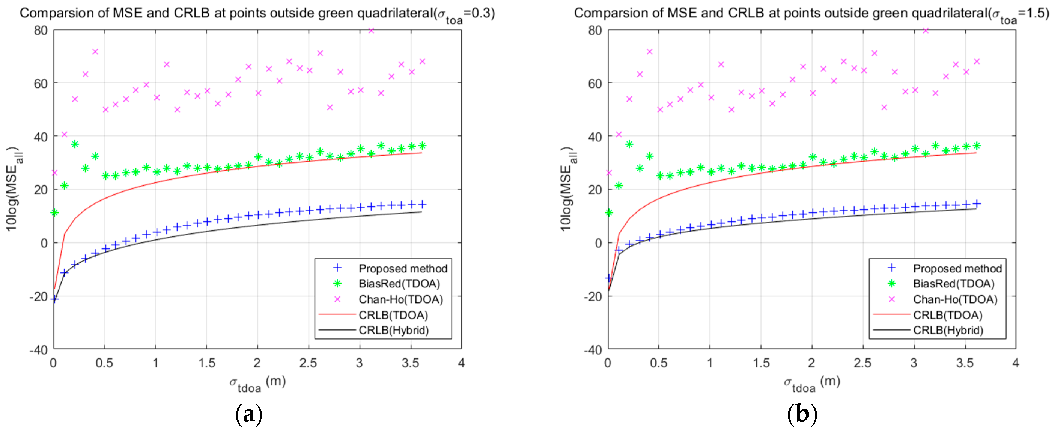
Figure 14 shows the
of positioning results and CRLBs at test points outside the green square. The result shows that the hybrid positioning has a lower CRLB than TDOA-only positioning. The
of the proposed algorithm approaches CRLB when TDOA ranging error is small. Even when the TDOA ranging error is higher, the positioning error of the proposed algorithm is also slightly higher than the CRLB and is significantly lower than the other two TDOA-only positioning methods. The positioning results of the proposed algorithm with
m are slightly better than it with
m when the standard deviation of TDOA ranging error is around 0.5 m.
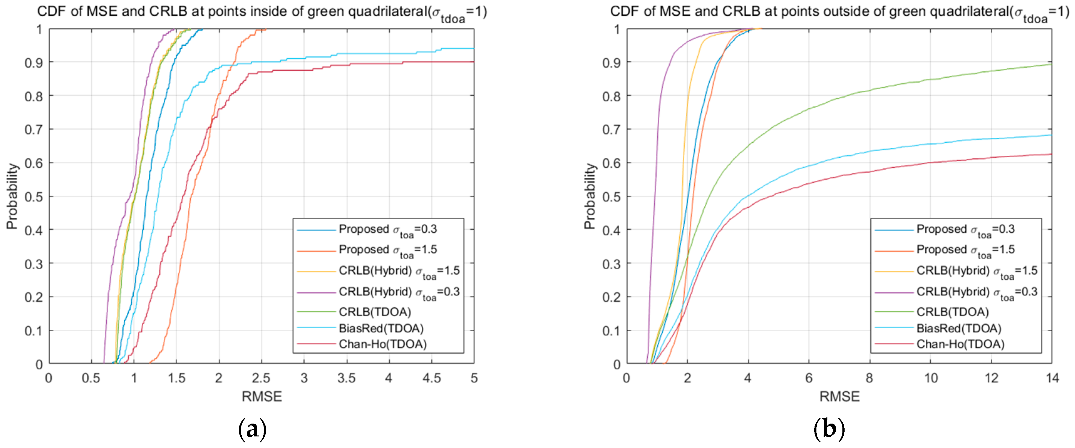
The algorithms performance at each selected points in
Figure 4 is also simulated as in
Section 5.2.1. Different from
Section 5.2.1, the square roots of MSE, called the root mean square error (RMSE), for different algorithms at every selected point are calculated. The CDF of the RMSE for the Chan-Ho, BiasRed, proposed algorithm with
m, proposed algorithm with
m and CRLBs are shown in
Figure 15, when
m.
As shown in
Figure 15b, it is obviously that, regardless of
or
m, performance of proposed algorithm is better than Chan-Ho and BiasRed algorithms. Only at 16% points, BiasRed algorithm is more accurate than the proposed algorithm when
m. Moreover, the Chan-Ho algorithm is only more accurate at 13% points compared to the proposed algorithm when
m. When
m, the proposed algorithm has a better performance than the two algorithms at all points outside the green quadrilateral. In
Figure 15a, the proposed algorithm still has a better performance than the two algorithms at all points inside the green quadrilateral when
m. In the comparison, the two algorithms and the proposed algorithm with
have their own advantages. BiasRed is more accurate than the proposed algorithm with
at 89% points and Chan-Ho is more accuracy than the proposed algorithm with
at 72% points. However, the proposed algorithm with
is more reliable than the two algorithm, since the maximum RMSE is only 2.613 and is much lower than the maximum RMSE of the two algorithms.
Based on the simulation results at the two groups’ points and the three selected test points, the proposed closed-form localization algorithm using multiple TDOAs and single TOA could provide a better positioning accuracy than the two closed-form TDOA-only positioning methods, Chan-Ho and BiasRed, in the indoor distribution system application scenario.
6. Conclusions
The 5G system could provide accurate multiple TDOA measurements and single TOA measurement, which could improve UE positioning accuracy. However, existing closed-form localization algorithms are designed for measurements having the same variance, and not suitable for heteroscedastic TDOA and TOA measurements.
In this paper, a three-step WLS closed-form localization algorithm is developed for the nonlinear equation set of those hybrid heteroscedastic measurements. The algorithm is an extension of Chan-Ho algorithm [
17]. The first WLS provides an initial position for the last two steps. Then the algorithm uses two WLSs to estimate position based on heteroscedastic TDOA and TOA measurements. Moreover, after the GDOP of this hybrid positioning is derived, it was proven that this hybrid positioning has a higher theoretical higher bound of accuracy than TDOA-only positioning.
The simulation scenario is built according to the real situation. By comparing with two TDOA-only closed-formed localization algorithm, Chan-Ho [
17] and BiasRed [
18], and CRLB [
35] of TDOA-only positioning and the proposed hybrid positioning in the same simulation scenario, the results show that the proposed localization algorithm has better performance than the two closed-form TDOA-only positioning methods, and the positioning accuracy approaches CRLB when the TDOA measurement errors are small. In different areas of the scenario, the proposed positioning algorithm has a different improvement in positioning accuracy. In the area surrounded by the ANTs, the proposed algorithm shows only a slight improvement effect. However, in the rest of the area, the accuracy of the proposed algorithm is even higher than the CRLB of TDOA-only positioning. The simulations indicates that using the hybrid TDOA and TOA measurements as well as the localization algorithm proposed in this paper have the potential to effectively improve the positioning accuracy of the indoor distribution system.
The proposed localization algorithm and the two compared algorithms, Chan-Ho and BiasRed, were constructed and simulated according to the ranging errors under the line-of-sight wireless propagation channel. In real scenes, non-line-of-sight channels are ubiquitous, which may cause the positioning accuracy of these algorithms to decrease. In future work, the analysis and improvement of the proposed algorithm in the non-line-of-sight environment can be studied. Meanwhile, the proposed algorithm is only confirmed by simulation for a specific environment. The actual algorithm performance should be investigated in future work.

