Photon Counting Statistics of a Microwave Cavity Coupled with Double Quantum Dots

Abstract

The statistical properties of photon emission counting, especially the waiting time distributions (WTDs) and large deviation statistics, of a cavity coupled with the system of double quantum dots (DQDs) driven by an external microwave field were investigated with the particle-number-resolved master equation. The results show that the decay rate of the WTDs of the cavity for short and long time limits can be effectively tuned by the driving external field Rabi frequency, the frequency of the cavity photon, and the detuning between the microwave driving frequency and the energy-splitting of the DQDs. The photon emission energy current will flow from the thermal reservoir to the system of the DQDs when the average photon number of the cavity in a steady state is larger than that of the thermal reservoir; otherwise, the photon emission energy current will flow in the opposite direction. This also demonstrates that the effect of the DQDs can be replaced a thermal reservoir when the rate difference of a photon absorbed and emitted by DQDs is larger than zero; otherwise, it is irreplaceable. The results deepen our understanding of the statistical properties of photon emission counting. It has a promising application in the construction of nanostructured devices of photon emission on demand and of optoelectronic devices.

1. Introduction

Counting statistics is now at the center of attention in the quantum statistical description of a given process, counting the random number of events up to a given point. For example, one can count up to a given time the number of photons emitted by a quantum optical system and the number of electrons transported through a nanoscopic structure. The distribution of waiting times between elementary physical events is an important tool to investigate temporal correlations and the counting statistics of stochastic processes [1]. Short-time physics and correlations can be described by waiting time distributions (WTDs), which give the distribution of the time interval between two successive events. Additionally, most counting statistical properties can be obtained from the WTDs alone in Markovian and renewal systems [2]. WTDs play a significant role in various branches of science and technology—for instance, in quantum optics [3,4] and nanososcopic electron transport [5,6]. Moreover, the theory of large deviations (LD) is concerned with the exponential decay of probabilities of large fluctuations in random systems. For a long time limit, the measurement of random systems will focus around the average value, and large deviations away from this value are exponentially suppressed [7]. The LD method provides a deep description of a stochastic counting process, and it can be applied to characterize photon counting processes in different quantum optical systems [8,9] and electron transport properties through mesoscopic conductors [10,11]. WTDs and the LD method are particularly useful and represent a fundamental theory and tools in investigating nanososcopic devices.

Experimentally, obtaining all cumulants of photon or electron counting distribution requires time-resolved single-particle detection techniques. By capacitively coupling a single-electron transistor to a quantum dot (QD), real-time counting statistics has been carried out experimentally by detecting single electron tunneling through a quantum dot [12,13]. The single-electron detection has also been used to measure electron–electron interference in the QD system [14], as well as the full counting statistics of superconducting junctions [15]. Furthermore, full counting statistics and spin dynamics in a quantum dot have been investigated using resonance fluorescence [16]. Usually, most experiments have been carried out at ultralow temperatures in the milliKelvin range; however, recently, single-electron detection has begun to be operated at room temperature by the optical blinking of a nearby semiconductor nanocrystal [17]. As for the single photon detector, a quantum nondemolition detector for propagating microwave photons was realized [18]. Such single-photon detectors have a wide range of applications within quantum thermodynamics [19] and quantum information processing [20]. Further progress in the measurements of photon counting statistics in quantum coherent optics is anticipated in the coming years, and with the rapid progress in single-photon detection, the measurement of single photon counting statistics could soon be within reach.

Theoretically, Brandes was the first one to study the WTDs of mesoscopic quantum transport by defining jump operators from a quantum master equation [21]. To date, WTDs have been investigated for double-quantum dots [22,23], quantum dot spin-valves [24], non-Markovian transport [25], superconducting devices [26,27], and coherent conductors [6,28,29]. Recently, the photon counting statistical characteristics of photon emission from a microwave cavity, such as WTDs and LD statistics, have been investigated [30]. Furthermore, photon counting statistics for a microwave cavity with multiple heat baths have also been studied. It is found that WTDs contain information about few-photon processes, which cannot easily be extracted from standard correlation measurements, and the large-deviation statistics of the photon current are helpful in understanding earlier results of heat-transport statistics and work distributions. These results can be generalized to a microwave cavity coupled with nanoscopic devices.

On the other hand, a system of double quantum dots (DQDs) interacting through microwave resonators has been proposed, and it is thought that this setup can be used to entangle macroscopically separated electron transport, which has applications in nanoscale quantum information processing [31]. This also provides a new way to study light–matter interactions [32] and implement a QD laser [33]. Because semiconductor DQDs’ energy level differences and electron–photon coupling strength are electrically tunable, the interaction of photons and electrons in DQDs has been studied extensively in the circuit QED architecture, where the charge dipole of DQDs is coupled to a microwave cavity.

In this paper, the photon counting statistics of a microwave cavity coupled with double quantum dots will be investigated. The influences of DQDs on the WTDs and LD statistics of a microwave cavity will be studied. The differences between a microwave cavity coupled with DQDs and coupled with a thermal bath are discussed. The photon emission counting statistical characteristics of the microwave cavity coupled with DQDs can be tunable because of the electrical tenability of the DQDs’ energy level differences and electron–photon coupling strength. The methods and results in this paper can also be applied to many similar quantum systems, such as opto-mechanics system and so on [34,35,36,37,38].

The paper is organized as follows. In Section 2, we present the model and theoretical formalism with a master equation, as well as WTDs and LD statistics. In Section 3, we study the effects of the driven microwave Rabi frequency, detuning between the microwave driving frequency and the DQDs energy-splitting and other parameters regarding the WTDs and LD statistics of photon emission. The conclusions will be given in Section 4.

2. Model and Theoretical Formalism

2.1. Hamiltonian Model

Figure 1 shows the system schematic of the DQDs with metal leads and the left quantum dot (QD) coupled to a one-mode microwave cavity, and each QD is modeled as a one-level system. An external driving microwave field has been applied between the two QDs; the vital advantage of this system is that one can adjust the gate voltage to tune both the energy-level splitting and the decay rate of the DQDs. The loss of the microwave cavity field is considered here by adding the interaction of the thermal bath and microwave cavity field.

In our DQD system, the distance between the two QDs is so small that only one electron can occupy the DQDs at a time. Thus, the states of DQDs can be presented as follows: $|0\rangle$ (vacuum state), $|1\rangle$ (the left dot occupied by one electron), $|2\rangle$ (the right dot occupied by one electron). The energy level difference of the two dots is $\hslash ℇ$ when the electron jumps from the left dot to the right induced by an external ac microwave field of frequency ${\omega }_d$ between the QDs. Adjusting the level difference $\hslash ℇ$ by the bias voltage to satisfy the condition ${\omega }_m=\epsilon -{\omega }_d$ (${\omega }_m$ is the frequency of microwave cavity field), the DQDs would absorb a photon of energy $\hslash \left(\epsilon -{\omega }_d\right)$ when an electron is excited from state $|1\rangle$ to state $|2\rangle$.

As shown in Figure 1b, the left chemical potential of lead is higher than that of the lead on the right. The total Hamiltonian of the whole system can be written as ($\hslash =1$) [39]

$$H=H_l+H_m+H_D+H_T+H_I.$$

(1)

The first term, $H_l$, describes the left and the right leads with a bias potential,

$$H_l={\displaystyle \sum _{\alpha k}{E}_{\alpha k}{c}_{\alpha k}^{†}}{c}_{\alpha k},$$

(2)

where the operator $c_{\alpha k}^{†}$ ($c_{\alpha k}$) creates (destroys) an electrode electron with momentum k in lead $\alpha =l$ or r (l = left, r = right), and $E_{\alpha k}$ describes the dispersion energy.

The second term, $H_m$, describes the energy of the microwave cavity field, which can be written as

$$H_m={\omega }_m{a}^{†}a,$$

(3)

where $a^{†}\left(a\right)$ is the microwave photon creation (annihilation) operator with frequency ${\omega }_m$.

The third term, $H_D$, describes the DQDs driven by the microwave photon field; i.e.,

$$H_D=\frac{\epsilon }{2}{\sigma }_z+\Omega {\sigma }_x+{\Omega }_0\cos \left({\omega }_{d}t\right){\sigma }_x,$$

(4)

where the operator ${\sigma }_z=d_2^{†}{d}_2-d_1^{†}{d}_1$ and ${\sigma }_x=d_2^{†}{d}_1+d_1^{†}{d}_2$ mean the Pauli matrices of the left or the right dot. The operator $d_1(d_2)$ stands for destroying an electron in the left (right) dot, $\epsilon$ is the energy-level difference of DQDs, $\mathsf{\Omega }$ is the tunneling strength between the two QDs [40], and ${\mathsf{\Omega }}_0$ is the Rabi frequency of the driving microwave field with driving frequency ${\omega }_d$ [40].

The fourth term, $H_T$, describes the tunneling coupling between the DQDs and electrode leads, so

$$H_T={\displaystyle \sum _k\left({\Omega }_{lk}{d}_1^{†}{c}_{lk}+{\Omega }_{rk}{d}_2^{†}{c}_{rk}+H.C\right)},$$

(5)

where ${\mathsf{\Omega }}_{lk }\left({\mathsf{\Omega }}_{rk}\right)$ denotes the coupling strength between the left (right) lead and the left (right) QD.

The interaction Hamiltonian $H_I$ between the left QD and the microwave cavity field is

$$H_I=-\lambda d_1^{†}{d}_1\left(a^{†}+a\right),$$

(6)

where $\lambda$ is the coupling between the cavity field and the electron in the left dot. $\lambda =\eta {\omega }_m$, $\eta$ is the scale of QD-cavity coupling strength. By performing a standard canonical transformation, $\tilde{H}=e^{s}H{e}^{-s}$ with $\mathrm{S}=-\eta \left(a^{†}-a\right)d_1^{†}{d}_1$, we obtain the transformed total Hamiltonian as

$$\begin{array}{l}\tilde{H}=e^{s}H{e}^{-s}\\ ={\displaystyle \sum _{\alpha k}{E}_{\alpha k}{c}_{\alpha k}^{†}}{c}_{\alpha k}+\frac{\epsilon }{2}{\sigma }_z+\left[\Omega +{\Omega }_0\cos \left({\omega }_{d}t\right)\right]\left({\sigma }_{+}{X}^{†}+H.C\right)\\ +{\omega }_{\mathrm{m}}{a}^{†}a+{\displaystyle \sum _k\left({\Omega }_{lk}{d}_1^{†}{c}_{lk}X+{\Omega }_{rk}{d}_2^{†}{c}_{rk}+H.C\right)}\end{array}$$

(7)

where $\mathrm{X}=\exp \left[-\eta \left(a^{†}-a\right)\right]$, ${\sigma }_{+}=d_2^{†}{d}_1, {\sigma }_{-}=d_1^{†}{d}_2$. Here, we introduce a unitary transform $\mathrm{U}=\exp \left\{-i\frac{{\omega }_d}{2}{\sigma }_{z}t\right\}$ to eliminate the driving term, and, under the rotating-wave approximation (${\omega }_d\gg \mathsf{\Omega }$), the final total Hamiltonian becomes

$$H_f=H_{sys}+{\displaystyle \sum _{\alpha k}{E}_{\alpha k}{c}_{\alpha k}^{†}}{c}_{\alpha k}+{\displaystyle \sum _k\left({\Omega }_{lk}{d}_1^{†}{c}_{lk}X{\mathrm{e}}^{-i\frac{{\omega }_d}{2}t}+{\Omega }_{rk}{d}_2^{†}{c}_{rk}{\mathrm{e}}^{i\frac{{\omega }_d}{2}t}+H.C\right)}$$

(8)

with

$$H_{sys}=-\frac{\Delta }{2}{\sigma }_z+{\omega }_{\mathrm{m}}{a}^{†}a+\frac{{\Omega }_0}{2}\left({\sigma }_{+}{X}^{†}+H.C^{}\right),$$

(9)

where $\mathsf{\Delta }={\omega }_d-\epsilon$ is the detuning between the microwave driving frequency and the energy-splitting of the DQDs.

2.2. Master Equation

Considering the Born–Markov approximation and tracing out the electrode lead reservoirs, one can obtain the system equation of the DQDs and the microwave cavity as follows [39]:

$$\frac{d}{dt}{\rho }_S=-i\left[H_{sys},{\rho }_S\right]+{ℒ}_T\rho +{ℒ}_D\rho ,$$

(10)

where the middle-term ${ℒ}_T\rho$ stands for the tunneling effect between DQDs and leads, and the last term ${ℒ}_D\rho$ expresses the dissipation term of the microwave cavity induced by the thermal reservoir; i.e.,

$$\begin{gathered} {ℒ}_T\rho ={\mathsf{\Gamma }}_r\mathcal{D}\left[d_2\right]{\rho }_s+{\Gamma }_l\left(1-{\eta }^2\right)\mathcal{D}\left[d_1^{†}\right]{\rho }_s+{\Gamma }_l{\eta }^2\left\{a^{†}a\left[d_1,d_1^{†}{\rho }_s\right]+\left[{\rho }_s{d}_1,d_1^{†}\right]a^{†}a\right\} \\ +{\Gamma }_l{\eta }^2\left\{\mathcal{D}\left[a^{†}{d}_1^{†}\right]{\rho }_s+\mathcal{D}\left[a{d}_1^{†}\right]{\rho }_s\right\}, \end{gathered}$$

(11)

$$\begin{array}{l}{ℒ}_D\rho =\frac{\gamma }{2}\left[1+\overline{n}\right]\left[2a{\rho }_S{a}^{†}-a^{†}a{\rho }_S-{\rho }_S{a}^{†}a\right]\\ +\frac{\gamma }{2}\overline{n}\left[2a^{†}{\rho }_{S}a-a{a}^{†}{\rho }_S-{\rho }_{S}a{a}^{†}\right]\end{array}$$

(12)

Here, we take operator X referred to above to expand up to the second order in η and assume that the energy levels with one microwave cavity photon mediating tunneling every time are in the bias window. Additionally, ${\Gamma }_{\alpha }={\displaystyle \sum }_{k}2\pi {\rho }_{\alpha k}{\Omega }_{\alpha k}^2$, ${\Gamma }_{\alpha }$. describes the tunneling rate of the electron from the lead α, while ${\rho }_{\alpha k}$ describes the density of the electron state with momentum k at lead α. The latter γ is the dissipation of the microwave cavity field, where $\overline{n}$ is the boson number in the thermal reservoir. Super-operator D has the following form: $D\left[A\right]\rho =A\rho A^{†}-\frac{1}{2}\left[A^{†}A\rho +\rho A^{†}A\right]$, A is the arbitrary operator.

Assuming the dissipation of the cavity field is smaller than the decay of the DQDs, the freedom of the DQDs could be eliminated as it is considered as an environment. Since we are interested in the behavior of the system in the limit $\mathrm{t}\to \infty$, applying the projecting operator method to calculate the density of the cavity, we can obtain the final master equation of the cavity field after taking the same approximation as used in [39]:

$$\begin{array}{ll}\frac{d}{dt}\mu =& i{\delta }_m\left[a^{†}a,\mu \right]+\frac{1}{2}\left[\gamma \left[1+\overline{n}\right]+A_{-}\left({\omega }_m\right)\right]\left[2a\mu a^{†}-a^{†}a\mu -\mu a^{†}a\right]\\ & +\frac{1}{2}\left[\gamma \overline{n}+A_{+}\left({\omega }_m\right)\right]\left[2a^{†}\mu a-a{a}^{†}\mu -\mu a{a}^{†}\right]\end{array}$$

(13)

where

$$\begin{array}{l}{\delta }_m={\eta }^2\frac{{\Omega }_0}{2}\langle {\sigma }_x\rangle -\mathrm{Im}\left[S\left({\omega }_m\right)+\left[S\left(-{\omega }_m\right)\right]\right]\\ A_{-}\left({\omega }_m\right)=2\mathrm{Re}\left[S\left({\omega }_m\right)\right]+2D\\ A_{+}\left({\omega }_m\right)=A_{-}\left(-{\omega }_m\right)\\ D=\frac{1}{2}{\eta }^2\langle {\rho }_d^0\rangle {\displaystyle \sum _{\sigma }{\Gamma }_{l\sigma }}\end{array}$$

(14)

The operator $\langle {\rho }_d^0\rangle$ describes the stationary probability of the DQDs in the empty state, μ stands for density matrix of microwave cavity field, ${\delta }_m$ is the driving-induced frequency shift, and $A_{\pm }$ shows the rates induced by the interaction between DQDs and cavity; moreover,

$$\mathrm{S}\left({\omega }_m\right)=\frac{{\eta }^2{\Omega }_0^2}{4}{\displaystyle {\int }_0^{\infty }dt}{e}^{i{\omega }_{m}t}\langle {\sigma }_y\left(t\right){\sigma }_y\left(0\right)\rangle ,$$

(15)

where $\langle {\sigma }_y\left(t\right){\sigma }_y\left(0\right)\rangle$ can be obtained via the quantum regression theorem. $\langle \cdots \rangle$ represents the quantum average of the DQDs degrees.

Under the condition of the steady state, the density motion equation of the DQDs can be written as

$$\frac{d{\rho }_d}{dt}=-i\left[-\frac{\Delta }{2}{\sigma }_{\mathrm{z}}+\frac{{\Omega }_0}{2}{\sigma }_x,{\rho }_d\right]+{\Gamma }_l\mathcal{D}\left[d_1^{†}\right]{\rho }_d+{\Gamma }_r\mathcal{D}\left[d_2\right]{\rho }_d.$$

(16)

2.3. Photon Emission Counting Statistics

To keep track of the number m of photons emitted into the thermal reservoir from the microwave cavity, the m-resolved state density matrices $\mu \left(m,t\right)$ can be written as [30]

$$\begin{array}{l}\frac{d}{dt}\mu (m,t)=\frac{1}{2}\gamma \left[1+\overline{n}\right]\left[2a\mu (m-1,t)a^{†}-\left\{a^{†}a,\mu (m,t)\right\}\right]+\frac{1}{2}\gamma \overline{n}\left[2a^{†}\mu (m,t)a-\left\{a^{†}a,\mu (m,t)\right\}\right]+\\ \hspace{1em}\hspace{1em}i{\delta }_m\left[{\mathrm{a}}^{†}a,\mu (m,t)\right]+\frac{1}{2}{A}_{+}\left[2a^{†}\mu (m,t)a-\left\{a^{†}a,\mu (m,t)\right\}\right]+\frac{1}{2}{A}_{-}\left[2a\mu (m,t)a^{†}-\left\{a^{†}a,\mu (m,t)\right\}\right]\end{array}$$

(17)

The probability of m photons being emitted from the cavity to the thermal reservoir can be obtained through $P\left(m,t\right)=\mathrm{Tr}\mu \left(m,t\right)$. If we perform the following Laplace transformation $\mu \left(\mathrm{s},\mathrm{t}\right)\equiv {\sum }_{m=0}^{\infty }\mu \left(m,t\right)e^{ms}$, Equation (17) can be transformed into

$$\begin{array}{l}\frac{d}{dt}\mu (s,t)=\frac{1}{2}\gamma \left[1+\overline{n}\right]\left[2e^{s}a\mu (s,t)a^{†}-\left\{a^{†}a,\mu (s,t)\right\}\right]+\frac{1}{2}\gamma \overline{n}\left[2a^{†}\mu (s,t)a-\left\{a^{†}a,\mu (s,t)\right\}\right]+\\ \hspace{1em}\hspace{1em}i{\delta }_m\left[{\mathrm{a}}^{†}a,\mu (s,t)\right]+\frac{1}{2}{A}_{+}\left[2a^{†}\mu (s,t)a-\left\{a^{†}a,\mu (s,t)\right\}\right]+\frac{1}{2}{A}_{-}\left[2a\mu (s,t)a^{†}-\left\{a^{†}a,\mu (s,t)\right\}\right]\end{array}$$

(18)

where s is called a counting field. In order to obtain the matrix elements $\langle n\left|\mu \left(s,t\right)\right|n\rangle$, we introduce another Laplace transformation as follows:

$$\mathcal{G}\left(\mathrm{s},\mathrm{q},\mathrm{t}\right)\equiv {\sum }_{n=0}^{\infty }\langle n\left|\mu \left(s,t\right)\right|n\rangle e^{nq}.$$

(19)

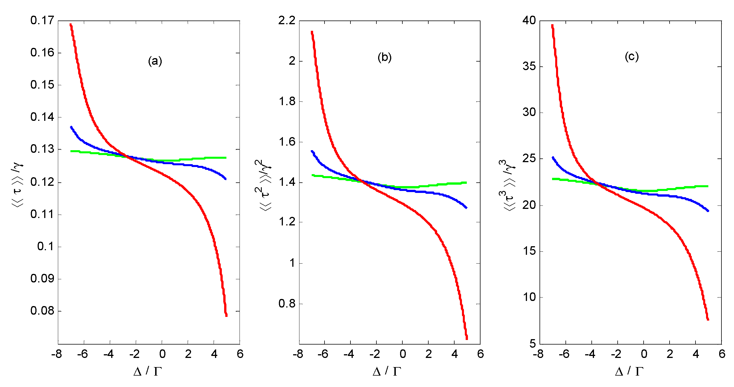
2.3.1. Waiting Time Distributions and Large-Deviation Statistics for Photon Emission

Using the method of characteristics [41], one can find the moment generating function (MGF) $ℳ\left(\mathrm{s},\mathrm{t}\right)=\mathrm{Tr}\mu \left(\mathrm{s},\mathrm{t}\right)$ as follows:

$$ℳ\left(\mathrm{s},\mathrm{t}\right)=\frac{2\xi e^{\left(\gamma +W\right)t/2}}{2\xi \cosh \left[\frac{\xi \left(\gamma +W\right)t}{2}\right]+\left(1+{\xi }^2\right)\sinh \left[\frac{\xi \left(\gamma +W\right)t}{2}\right]},$$

(20)

where $\xi =\sqrt{1-4{\overline{n}}_c\left(1+\overline{n}\right)\left(e^s-1\right)/\left(1+W/\gamma \right)}$, $W=A_{-}-A_{+}$. ${\overline{n}}_c=\left(\gamma \overline{n}+A_{+}\right)/\left(\gamma +W\right)$ is the average photon number of the cavity in a steady state. The waiting time distributions for waiting time τ between each two photon emissions can be calculated with [42]:

$$\mathcal{W}\left(\mathsf{\tau }\right)={\partial }_{\mathsf{\tau }}^2\mathsf{\Pi }\left(\mathsf{\tau }\right)/p,$$

(21)

where $\mathsf{\Pi }\left(\mathsf{\tau }\right)=ℳ\left(-\infty ,\mathsf{\tau }\right)$, $p=-{\partial }_{\mathsf{\tau }}\mathsf{\Pi }\left(\mathsf{\tau }\right){|}_{\mathsf{\tau }=0}$.

Thus, we can obtain

$$\mathcal{W}\left(\mathsf{\tau }\right)=\overline{\mathsf{\Gamma }}\left(\gamma +W\right)\overline{\gamma }\frac{\gamma +W+6\overline{\mathsf{\Gamma }}+\left(\gamma +W+2\overline{\mathsf{\Gamma }}\right)\cosh \left[\overline{\gamma }t\right]+\overline{\gamma }\sinh \left[\overline{\gamma }t\right]}{\overline{\gamma }\cosh \left[\frac{\overline{\gamma }t}{2}\right]+\left(\gamma +W+2\overline{\mathsf{\Gamma }}\right)\sinh \left[\frac{\overline{\gamma }t}{2}\right]}{e}^{\left(\gamma +W\right)t/2},$$

(22)

where $\overline{\gamma }=\left(\gamma +\mathrm{W}\right)\sqrt{1+4{\overline{n}}_c\left(1+\overline{n}\right)/\left(1+W/\gamma \right)}$, $\overline{\mathsf{\Gamma }}=\gamma \left(1+\overline{\mathrm{n}}\right){\overline{n}}_c$.

For the long time limit, the cumulant generating function $\mathsf{\Theta }\left(\mathrm{s}\right)$ for the photon emission current is

$$\mathsf{\Theta }\left(\mathrm{s}\right)=\underset{\mathrm{t}\to \infty }{\lim }\frac{\ln ℳ\left(s,t\right)}{t}=\frac{\gamma +W}{2}\left\{1-\sqrt{1-4\frac{\gamma }{{\left(\gamma +W\right)}^2}k\left(s\right)}\right\},$$

(23)

where $k\left(\mathrm{s}\right)=(A_{+}+\gamma \overline{n})\left(1+\overline{n}\right)\left(e^s-1\right)$.

The probability $P\left(J,t\right)$ can be extracted as a Fourier coefficient of the MGF [30]:

$$P\left(\mathrm{J},\mathrm{t}\right)=\frac{1}{2\pi i}{\int }_{-\pi }^{\pi }ℳ\left(s,\mathsf{\tau }\right)e^{-ms}ds=\frac{1}{2\pi i}{\int }_{-i\pi }^{i\pi }{e}^{t\left[\mathsf{\Theta }\left(s\right)-Js\right]}ds,$$

(24)

where J = m/t. For the long time limit, this integral can be solved using the saddle-point approximation. Let $s_0$ be the solution to the saddle-point equation ${\mathsf{\Theta }}^{\prime }\left(s_0\right)=J$. The integral in Equation (24) can be performed explicitly, meaning that we can get

$$\frac{\ln \left[P\left(J,t\right)\right]}{t}\approx \mathsf{\Theta }\left(s_0\right)-J{s}_0,$$

(25)

$$\begin{gathered} \frac{\ln \left[P\left(J,t\right)\right]}{t}\approx \frac{\gamma +W}{2}+J-\frac{\sqrt{4J^2+{\left(\gamma +W\right)}^2+4\gamma \left(\gamma +W\right){\overline{n}}_c\left(1+\overline{n}\right)}}{2} \\ +\mathrm{J}\ln \frac{\gamma \left(\gamma +W\right){\overline{n}}_c\left(1+\overline{n}\right)}{J\left[\sqrt{4J^2+{\left(\gamma +W\right)}^2+4\gamma \left(\gamma +W\right){\overline{n}}_c\left(1+\overline{n}\right)}-2J\right]}. \end{gathered}$$

(26)

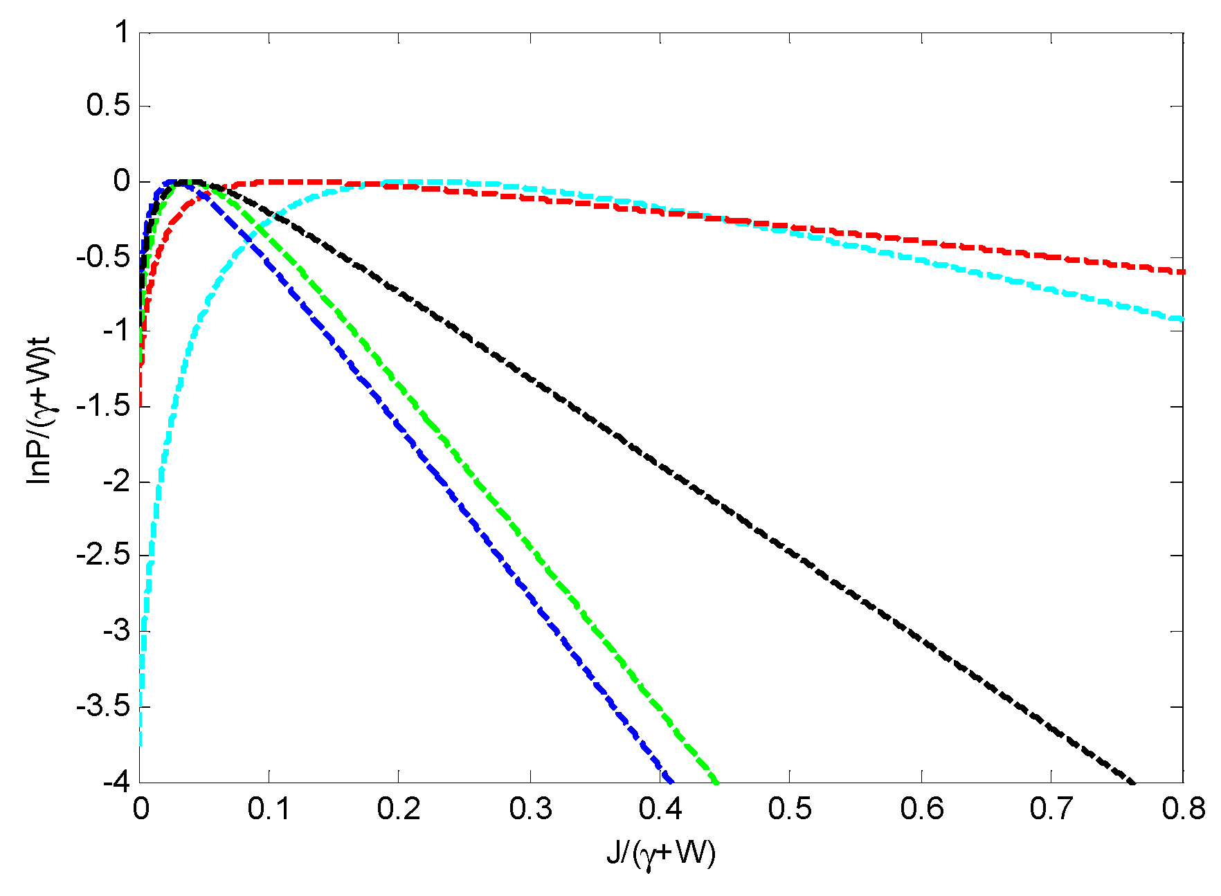
2.3.2. Large-Deviation Statistics for Net Photon Current

If we investigate the net photon current statistics between the cavity and the thermal reservoir, Equation (18) can be rewritten as

$$\begin{array}{l}\frac{d}{dt}\mu (s,t)=\frac{1}{2}\gamma \left[1+\overline{n}\right]\left[2e^{s}a\mu (s,t)a^{†}-\left\{a^{†}a,\mu (s,t)\right\}\right]+\frac{1}{2}\gamma \overline{n}\left[2e^{-s}{a}^{†}\mu (s,t)a-\left\{a^{†}a,\mu (s,t)\right\}\right]+\\ \hspace{1em}\hspace{1em}i{\delta }_m\left[{\mathrm{a}}^{†}a,\mu (s,t)\right]+\frac{1}{2}{A}_{+}\left[2a^{†}\mu (s,t)a-\left\{a^{†}a,\mu (s,t)\right\}\right]+\frac{1}{2}{A}_{-}\left[2a\mu (s,t)a^{†}-\left\{a^{†}a,\mu (s,t)\right\}\right]\end{array}$$

(27)

Then, the moment generating function can be obtained as

$$ℳ\left(\mathrm{s},\mathrm{t}\right)=\frac{2\xi e^{\left(\gamma +W\right)t/2}}{2\xi \cosh \left[\frac{\xi \left(\gamma +W\right)t}{2}\right]+\left(1+{\chi }^2\right)\sinh \left[\frac{\xi \left(\gamma +W\right)t}{2}\right]},$$

(28)

where

$$\begin{gathered} \xi =\sqrt{1-4\left[A_{+}\left(1+\overline{n}\right)\left(e^s-1\right)+A_{-}\overline{n}\left(e^{-s}-1\right)\right]/{\left(1+W/\gamma \right)}^2} \\ \chi =\sqrt{1-4\left[\left(1+\overline{n}\right){\overline{n}}_c\left(e^s-1\right)+\left(1+{\overline{n}}_c\right)\overline{n}\left(e^{-s}-1\right)\right]/\left(1+W/\gamma \right)}. \end{gathered}$$

(29)

For the long time limit, the cumulant generating function $\mathsf{\Theta }\left(\mathrm{s}\right)$ for the net photon current is

$${\mathsf{\Theta }}_{net}\left(\mathrm{s}\right)=\underset{\mathrm{t}\to \infty }{\lim }\frac{\ln ℳ\left(s,t\right)}{t}=\frac{\gamma +W}{2}\left\{1-\sqrt{1-4\frac{\gamma }{{\left(\gamma +W\right)}^2}k\left(s\right)}\right\},$$

(30)

where $k\left(\mathrm{s}\right)=A_{+}\left(1+\overline{n}\right)\left(e^s-1\right)+A_{-}\overline{n}\left(e^{-s}-1\right)$. The probability $P\left(J,t\right)$ can be obtained as

$$\frac{\ln \left[P\left(J,t\right)\right]}{t}\approx {\mathsf{\Theta }}_{net}\left(s_0\right)-J{s}_0,$$

(31)

where ${\mathsf{\Theta }}_{net}^{\prime }\left(s_0\right)=J$.

3. Discussion

From Equation (17), one can find that the parameters $A_{+}$ and $A_{-}$ represent the influence of DQDs on the density matrix of the microwave cavity. $A_{+}$ is the rate of the photon emitted from DQDs to the cavity and $A_{-}$ is the rate of the photon absorbed by DQDs from the cavity. It can be found that, if $\gamma +\mathrm{W}<0$, the average phonon occupancy of the cavity can be increased to infinity and has no stationary solution. In contrast, for $\gamma +\mathrm{W}>0$, one can reach a steady state. The average photon number of the cavity in a steady state is ${\overline{n}}_c=\left(\gamma \overline{n}+A_{+}\right)/\left(\gamma +W\right)$.

Firstly, we investigate the variation range of the parameters $A_{+}$ and $A_{-}$, and the influence on the average photon number ${\overline{n}}_c$. The parameters in this paper are assumed with reference to the typical experimental parameters [43,44]. In Figure 2, the parameters $W=A_{-}-A_{+}$, $A_{+}$ and ${\overline{n}}_c$ are plotted as a function of the driving detuning $\mathsf{\Delta }={\omega }_d-\epsilon$ for different driving Rabi frequencies of the external microwave field. This shows that the sign of the W exhibits a dependence on the detuning. W is at maximum when $\mathsf{\Delta }<0$ and at minimum when $\mathsf{\Delta }>0$, while $A_{+}$ is at a maximum when $\mathsf{\Delta }>0$. One can also find that the average photon number of the microwave cavity in a steady state is at minimum when W is at maximum and it increases to infinity when $W<0$. Additionally, ${\overline{n}}_c$ could be less than the photon number $\overline{n}$ of the thermal reservoir when $W>0$, while it could be more than $\overline{n}$ when $W<0$. Figure 2 also shows that the parameters $W$, $A_{+}$ and ${\overline{n}}_c$ are dependent on the driving Rabi frequency.

Figure 3 demonstrates the WTDs for different parameters. The black line exhibits the WTD of the cavity without the DQD system. It can be found that all the WTDs start off at a finite value, $W\left(\mathsf{\tau }\right)\approx 2\overline{\mathsf{\Gamma }}{e}^{-\left[6\frac{\gamma {\overline{n}}_c\left(1+\overline{n}\right)}{\gamma +W}+1\right]\left(\gamma +W\right)\mathsf{\tau }/2}$ ($\overline{\mathsf{\Gamma }}\mathsf{\tau }\ll 1$), and then decay exponentially to zero over long times, $W\left(\mathsf{\tau }\right)\approx \frac{4\overline{\mathsf{\Gamma }}\overline{\gamma }\left(\gamma +W\right)}{{\left(\gamma +W+\overline{\gamma }+2\overline{\mathsf{\Gamma }}\right)}^2}{e}^{-\left(\sqrt{1+4{\overline{n}}_c\gamma \left(1+\overline{n}\right)/\left(\gamma +W\right)}-1\right) \left(\gamma +W\right)\mathsf{\tau }/2}$ ($\overline{\mathsf{\Gamma }}\mathsf{\tau }\gg 1$). Comparing the green line to the black line, one can find that, when detuning $\mathsf{\Delta }=-4\mathsf{\Gamma }$, the WTD of the cavity coupled with DQDs is very close to that of a cavity without DQDs because the average photon number of the cavity ${\overline{n}}_c=0.85$ is very close to that of the thermal reservoir. The cyan line and red line show that the decay rate of $\mathsf{\Delta }=5.5\mathsf{\Gamma }$ is very different from that of the DQDs replaced by a thermal bath, with ${\overline{n}}_h=10$ for the long time limit, although these two decay rates are very close to each other for a short time range.

Figure 4 shows the first-order, second-order, and third-order cumulants of waiting time as a function of detuning with different driving Rabi frequencies and microwave cavity frequencies. From Figure 2 and Figure 4, it can be found that the cumulants of waiting time vary abruptly in the vicinity of the maximum of W, and the cumulants vary much more steeply if W has a larger maximum as detuning varies. Overall, the waiting time statistical properties can be tuned by the parameters of the DQD system.

Figure 5 demonstrates the large-deviation statistics of the photon emission current from the cavity to the thermal reservoir as a function of the photon emission current J. From Figure 5, we can find that the distributions become strongly non-Poissonian and large emission currents are more likely as the average photon number of the cavity ${\overline{n}}_c$ increases when adjusting the parameters of the DQD system. If ${\overline{n}}_c$ > $\overline{n}$, a large emission current is more likely than that of a cavity without DQDs; otherwise, it is less likely. Comparing the cyan line and red line, we find that the probability of small and large emission currents of $\mathsf{\Delta }=5\mathsf{\Gamma }$ are higher than those of DQDs replaced with a thermal reservoir with ${\overline{n}}_h=10$, although ${\overline{n}}_c=3$ for $\mathsf{\Delta }=5\mathsf{\Gamma }$ while ${\overline{n}}_c=5.5$ for DQDs replaced with a thermal reservoir. This reflects the fact that large-deviation statistics are not only dependent on the parameter $A_{+}$, but also dependent on the parameters $A_{-}$ and W.

Figure 6 exhibits large-deviation statistics of the net photon emission current as a function of the net photon emission current J from the cavity to reservoir. From the black line, we see that the probability of the photon emission energy current moving from the cavity to the thermal reservoir is the same as that of the photon emission current from the thermal reservoir to the cavity because the system is in steady state. The blue line and green line show that, if average photon number of the cavity satisfies the condition ${\overline{n}}_c$ > $\overline{n}$, the photon emission energy current will flow from the thermal reservoir to the system of the DQDs; otherwise, the photon emission energy current will flow in the opposite direction. As for the red line ($\mathsf{\Delta }=5\mathsf{\Gamma }$, W < 0) and the magenta line ($\mathsf{\Delta }=0,W=0$), the photon emission current from the thermal reservoir to the cavity are suppressed, which is quite different from that of the other cases. In particular, the most probable photon emission current is shifted from zero to a positive photon emission current J for the red line ($\mathsf{\Delta }=5\mathsf{\Gamma }$, W < 0).

From all of the above discussion, we find that the statistical properties of the photon emission counting of a cavity coupled with DQDs are similar to those of a cavity coupled with another thermal reservoir instead of DQDs when W > 0; otherwise, these statistical properties are quite different. This is because the effect of the DQDs on the photon emission counting statistical properties is the same as that of a thermal reservoir with ${\gamma }_h=W,{\overline{n}}_h=A_{+}/W$ when W > 0. If the parameters satisfy the condition W $\le$ 0, the effect of the DQDs cannot be replaced by that of a thermal reservoir. This is the essential characteristic of the system presented in this paper.

4. Conclusions and Remarks

In summary, we firstly employed Born–Markov approximation and the projecting operator method to obtain the reduced master equation of a cavity coupled with a system of DQDs which was driven by an external microwave field. Then, we investigated the influences of the parameters of DQDs on the photon emission counting statistical properties, especially the WTDs and large deviation statistics, of the cavity. The results show that the interaction between the DQDs and cavity has an obvious effect on the statistical properties of photon emission counting.

Firstly, the decay rates of WTDs of the cavity for short and long time limits—the cumulants of waiting time—can be effectively tuned by the driving external field Rabi frequency, the frequency of the cavity photon, the detuning between the microwave driving frequency, and the energy-splitting of the DQDs. Conversely, the state and properties of the DQDs can be extracted from WTDs and the cumulants of waiting time.

Secondly, the first-order, second-order and third-order cumulants of waiting time vary much more steeply if the rate W, which is the rate difference between a photon absorbed and emitted by DQDs, has larger maximum as the detuning varies.

Thirdly, the photon emission energy current will flow from the thermal reservoir to the system of the DQDs when the average photon number of the cavity in a steady state is larger than that of the thermal reservoir; otherwise, the photon emission energy current will flow in the opposite direction.

Finally, the effect of the DQDs and the effect of a thermal reservoir with ${\gamma }_h=W,{\overline{n}}_h=A_{+}/W$ on the photon emission counting statistical properties is the same when the rate difference of a photon absorbed and emitted by DQDs is larger than zero. If the rate difference between a photon absorbed and emitted by DQDs is less than or equal to zero, the effect of the DQDs cannot be replaced by that of a thermal reservoir.

On the whole, WTDs and the large-deviation statistics properties of a cavity can be strictly regulated and controlled by the parameters of the DQD system online. The effects of the DQDs on the statistical properties of photon emission counting are irreplaceable in certain parameter regions. Thus, these results deepen our understanding of the statistical properties of photon emission counting, enrich the control techniques for the photon emission of a cavity, and open a new door for the construction of nanostructured devices of photon emission on demand and optoelectronic devices.

References

1. Van Kampen, N.G. Stochastic Processes in Physics and Chemistry; Elsevier: Amsterdam, The Netherlands, 2007. [Google Scholar]
2. Cox, D.R. Renewal Theory; Chapman and Hall: London, UK, 1962. [Google Scholar]
3. Cohen-Tannoudji, C.; Dalibard, J. Single-atom laser spectroscopy. Looking for dark periods in fluorescence light. Europhys. Lett. 1986, 1, 441. [Google Scholar] [CrossRef]
4. Zoller, P.; Marte, M.; Walls, D.F. Quantum jumps in atomic systems. Phys. Rev. A 1987, 35, 198. [Google Scholar] [CrossRef] [PubMed]
5. Albert, M.; Flindt, C.; Büttiker, M. Distributions of waiting times of dynamic single-electron emitters. Phys. Rev. Lett. 2011, 107, 086805. [Google Scholar] [CrossRef] [PubMed]
6. Albert, M.; Haack, G.; Flindt, C.; Büttiker, M. Electron waiting times in mesoscopic conductors. Phys. Rev. Lett. 2012, 108, 186806. [Google Scholar] [CrossRef] [PubMed]
7. Touchette, H. The large deviation approach to statistical mechanics. Phys. Rep. 2009, 478, 1–69. [Google Scholar] [CrossRef]
8. Garrahan, J.P.; Lesanovsky, I. Thermodynamics of quantum jump trajectories. Phys. Rev. Lett. 2010, 104, 160601. [Google Scholar] [CrossRef]
9. Xu, L.; Li, X.Q. Counting statistics of photon emissions detected in non-Markovian environment. Sci. Rep. 2018, 8, 531. [Google Scholar] [CrossRef]
10. Li, J.; Liu, Y.; Ping, J.; Li, S.S.; Li, X.Q.; Yan, Y. Large-deviation analysis for counting statistics in mesoscopic transport. Phys. Rev. B 2011, 84, 115319. [Google Scholar] [CrossRef]
11. Žnidarič, M. Large-deviation statistics of a diffusive quantum spin chain and the additivity principle. Phys. Rev. E 2014, 89, 042140. [Google Scholar] [CrossRef]
12. Lu, W.; Ji, Z.; Pfeiffer, L.; West, K.W.; Rimberg, A.J. Real-time detection of electron tunnelling in a quantum dot. Nature 2003, 423, 422. [Google Scholar] [CrossRef]
13. Fujisawa, T.; Hayashi, T.; Tomita, R.; Hirayama, Y. Bidirectional counting of single electrons. Science 2006, 312, 1634–1636. [Google Scholar] [CrossRef] [PubMed]
14. Gustavsson, S.; Leturcq, R.; Studer, M.; Ihn, T.; Ensslin, K.; Driscoll, D.C.; Gossard, A.C. Time-resolved detection of single-electron interference. Nano Lett. 2008, 8, 2547–2550. [Google Scholar] [CrossRef] [PubMed]
15. Maisi, V.F.; Kambly, D.; Flindt, C.; Pekola, J.P. Full counting statistics of Andreev tunneling. Phys. Rev. Lett. 2014, 112, 036801. [Google Scholar] [CrossRef] [PubMed]
16. Kurzmann, A.; Stegmann, P.; Kerski, J.; Schott, R.; Ludwig, A.; Wieck, A.D.; König, J.; Lorke, A.; Geller, M. Optical detection of single-electron tunneling into a semiconductor quantum dot. Phys. Rev. Lett. 2019, 122, 247403. [Google Scholar] [CrossRef]
17. Zbydniewska, E.; Duzynska, A.; Popoff, M.; Hourlier, D.; Lenfant, S.; Judek, J.; Zdrojek, M.; Mélin, T. Charge blinking statistics of semiconductor nanocrystals revealed by carbon nanotube single charge sensors. Nano Lett. 2015, 15, 6349–6356. [Google Scholar] [CrossRef]
18. Besse, J.C.; Gasparinetti, S.; Collodo, M.; Walter, T.; Kurpiers, P.; Eichler, C.; Wallraff, A. Single-shot quantum non-demolition detection of an itinerant microwave photons. Nat. Phys. 2018, 14, 546–549. [Google Scholar]
19. Vinjanampathy, S.; Anders, J. Quantum thermodynamics. Cont. Phys. 2016, 57, 545. [Google Scholar] [CrossRef]
20. Nielsen, M.A.; Chuang, I.L. Quantum Computation and Quantum Information; Cambridge University Press: Cambridge, UK, 2011. [Google Scholar]
21. Brandes, T. Waiting times and noise in single particle transport. Annalen der Physik 2008, 17, 477–496. [Google Scholar] [CrossRef]
22. Ptaszyński, K. Nonrenewal statistics in transport through quantum dots. Phys. Rev. B 2017, 95, 045306. [Google Scholar] [CrossRef]
23. Ptaszyński, K. Waiting time distribution revealing the internal spin dynamics in a double quantum dot. Phys. Rev. B 2017, 96, 035409. [Google Scholar] [CrossRef]
24. Sothmann, B. Electronic waiting-time distribution of a quantum-dot spin valve. Phys. Rev. B 2014, 90, 155315. [Google Scholar] [CrossRef]
25. Thomas, K.H.; Flindt, C. Electron waiting times in non-Markovian quantum transport. Phys. Rev. B 2013, 87, 121405. [Google Scholar] [CrossRef]
26. Rajabi, L.; Pöltl, C.; Governale, M. Waiting time distributions for the transport through a quantum-dot tunnel coupled to one normal and one superconducting lead. Phys. Rev. Lett. 2013, 111, 067002. [Google Scholar] [CrossRef] [PubMed]
27. Chevallier, D.; Albert, M.; Devillard, P. Probing Majorana and Andreev bound states with waiting times. Eurphys. Lett. 2016, 116, 27005. [Google Scholar] [CrossRef]
28. Dasenbrook, D.; Hofer, P.P.; Flindt, C. Electron waiting times in coherent conductors are correlated. Phys. Rev. B 2015, 91, 195420. [Google Scholar] [CrossRef]
29. Haack, G.; Albert, M.; Flindt, C. Distributions of electron waiting times in quantum-coherent conductors. Phys. Rev. B 2014, 90, 205429. [Google Scholar] [CrossRef]
30. Brange, F.; Menczel, P.; Flindt, C. Photon counting statistics of a microwave cavity. Phys. Rev. B 2019, 99, 085418. [Google Scholar] [CrossRef]
31. Deng, G.W.; Wei, D.; Li, S.X.; Johansson, J.R.; Kong, W.C.; Li, H.O.; Jiang, H.W. Coupling two distant double quantum dots with a microwave resonator. Nano Lett. 2015, 15, 6620–6625. [Google Scholar] [CrossRef]
32. Delbecq, M.R.; Schmitt, V.; Parmentier, F.D.; Roch, N.; Viennot, J.J.; Fève, G.; Huard, B.; Mora, C.; Cottet, A.; Kontos, T. Coupling a quantum dot, fermionic leads, and a microwave cavity on a chip. Phys. Rev. Lett. 2011, 107, 256804. [Google Scholar] [CrossRef]
33. Agarwalla, B.K.; Kulkarni, M.; Mukamel, S.; Segal, D. Giant photon gain in large-scale quantum dot-circuit QED systems. Phys. Rev. B 2016, 94, 121305. [Google Scholar] [CrossRef]
34. Liu, Y.L.; Wang, C.; Zhang, J.; Liu, Y.X. Cavity optomechanics: Manipulating photons and phonons towards the single-photon strong coupling. Chin. Phys. B 2018, 27, 024204. [Google Scholar] [CrossRef]
35. Zhang, J.Q.; Zhang, S.; Zou, J.H.; Chen, L.; Yang, W.; Li, Y.; Feng, M. Fast optical cooling of nanomechanical cantilever with the dynamical Zeeman effect. Opt. Express 2013, 21, 29695–29710. [Google Scholar] [CrossRef] [PubMed] [Green Version]
36. Li, Z.Z.; Ouyang, S.H.; Lam, C.H.; You, J.Q. Cooling a nanomechanical resonator by a triple quantum dot. Europhys. Lett. 2011, 95, 40003. [Google Scholar] [CrossRef] [Green Version]
37. Zhou, B.Y.; Li, G.X. Ground-state cooling of a nanomechanical resonator via single-polariton optomechanics in a coupled quantum-dot–cavity system. Phys. Rev. A 2016, 94, 033809. [Google Scholar] [CrossRef]
38. Xiong, W.; Jin, D.Y.; Qiu, Y.; Lam, C.H.; You, J.Q. Cross-Kerr effect on an optomechanical system. Phys. Rev. A 2016, 93, 023844. [Google Scholar] [CrossRef] [Green Version]
39. Ouyang, S.H.; You, J.Q.; Nori, F. Cooling a mechanical resonator via coupling to a tunable double quantum dot. Phys. Rev. B 2009, 79, 075304. [Google Scholar] [CrossRef] [Green Version]
40. Zhu, J.P.; Li, G.X. Ground-state cooling of a nanomechanical resonator with a triple quantum dot via quantum interference. Phys. Rev. A 2012, 86, 053828. [Google Scholar] [CrossRef]
41. Renardy, M.; Rogers, R.C. An Introduction to Partial Differential Equations, 2nd ed.; Springer: New York, NY, USA, 2004. [Google Scholar]
42. Rudge, S.L.; Kosov, D.S. Counting quantum jumps: A summary and comparison of fixed-time and fluctuating-time statistics in electron transport. J. Chem. Phys. 2019, 151, 034107. [Google Scholar] [CrossRef] [Green Version]
43. Stockklauser, A.; Scarlino, P.; Koski, J.V.; Gasparinetti, S.; Andersen, C.K.; Reichl, C.; Wegscheider, W.; Ihn, T.; Ensslin, K.; Wallraff, A. Strong coupling cavity QED with gate-defined double quantum dots enabled by a high impedance resonator. Phys. Rev. X 2017, 7, 011030. [Google Scholar] [CrossRef] [Green Version]
44. Gullans, M.J.; Taylor, J.M.; Petta, J.R. Probing electron-phonon interactions in the charge-photon dynamics of cavity-coupled double quantum dots. Phys. Rev. B 2018, 97, 035305. [Google Scholar] [CrossRef] [Green Version]
Figure 1. (a) The diagram shows the double quantum dots (DQDs) connected to symmetric leads: the left electrode is the electron source, and the right is the drain; between the two dots, a bias voltage is added. The left quantum dot is coupled with a microwave cavity by capacitive coupling. The level difference of the two dots is , and the electron jumping from the left dot to the right is driven by an external alternating current (AC) microwave field of frequency ω d between the two dots. (b) An electron tunnels from the source to the left quantum dot and is driven to the right dot by the microwave field, finally tunneling to the drain ( μ L > μ R ).
Applsci 09 04934 g001
Figure 2. (a) the rate W / γ as a function of the driving detuning Δ = ω d ε for different driving Rabi frequencies Ω 0 = 5 Γ (red line) and Ω 0 = 7 Γ (blue line); (b) A + / γ as a function of the driving detuning Δ for different driving Rabi frequencies Ω 0 = 5 Γ (red line) and Ω 0 = 7 Γ (blue line); (c) the average photon number of the cavity as a function of the driving detuning Δ for Ω 0 = 7 Γ ; (d) the average photon number of the cavity as a function of the driving detuning Δ for different driving Rabi frequencies, Ω 0 = 5 Γ (red line). γ = 0.02 , n ¯ = 1 , Γ l = Γ r = Γ = 1 , ω m = 10 Γ , η = 0.05 .
Applsci 09 04934 g002
Figure 3. (a) waiting time distribuitions (WTDs) as a function of waiting time τ for different parameters. Δ = 7 Γ (blue line); Δ = 4 Γ (green line); Δ = 5.5 Γ (red line); cavity without DQDs (black line); DQDs replaced by thermal bath γ h = 0.02 ,   n ¯ h = 10 (cyan), thermal bath γ h = 0.02 ,   n ¯ h = 0 (magenta); γ = 0.02 , n ¯ = 1 , Γ = 1 , ω m = 10 Γ , η = 0.05 , Ω 0 = 7 Γ ; (b) the same curves as (a) on a logarithmic scale.
Applsci 09 04934 g003
Figure 4. The first-order (a), second-order (b) and third-order (c) cumulants of waiting time as function of detuning. Ω 0 = 7 Γ , ω m = 10 Γ (red line); Ω 0 = 5 Γ , ω m = 10 Γ (blue line); Ω 0 = 5 Γ , ω m = 15 Γ (green line); γ = 0.02 , n ¯ = 1 , Γ = 1 , η = 0.05 .
Applsci 09 04934 g004
Figure 5. Large-deviation statistics of the photon emission current. Analytic results for the distribution of the photon emission current J from a cavity to reservoir with Δ = 5 Γ (blue line); Δ = 5 Γ (red line), cavity without DQDs (black line); DQDs replaced by thermal reservoir γ h = 0.02 , n ¯ h = 1 (green line), thermal bath γ h = 0.02 , n ¯ h = 10 (cyan); γ = 0.02 , n ¯ = 1 , Γ = 1 , ω m = 10 Γ , η = 0.05 , Ω 0 = 7 Γ .
Applsci 09 04934 g005
Figure 6. Large-deviation statistics of the net photon emission current. Numeric results for the distribution of the net photon emission current J from a cavity to reservoir with Δ = 5 Γ (blue line); Δ = 5 Γ (red line); Δ = 0 (magenta line); DQDs replaced by thermal reservoir γ h = 0.02 , n ¯ h = 1 (black line), thermal bath γ h = 0.02 , n ¯ h = 10 (green); γ = 0.02 , n ¯ = 1 , Γ = 1 , ω m = 10 Γ , η = 0.05 , Ω 0 = 7 Γ .
Applsci 09 04934 g006