Article

Scene Description for Visually Impaired People with Multi-Label Convolutional SVM Networks

1
Department of Computer Engineering, College of Computer and Information Sciences, King Saud University, Riyadh 11543, Saudi Arabia
2
Department of Information Engineering and Computer Science, University of Trento, via Sommarive 9, 38123 Trento, Italy
*
Author to whom correspondence should be addressed.
Appl. Sci. 2019, 9(23), 5062; https://doi.org/10.3390/app9235062
Submission received: 21 October 2019 / Revised: 19 November 2019 / Accepted: 21 November 2019 / Published: 23 November 2019
(This article belongs to the Special Issue Recent Advances in Indoor Localization Systems and Technologies)

Abstract

:
In this paper, we present a portable camera-based method for helping visually impaired (VI) people to recognize multiple objects in images. This method relies on a novel multi-label convolutional support vector machine (CSVM) network for coarse description of images. The core idea of CSVM is to use a set of linear SVMs as filter banks for feature map generation. During the training phase, the weights of the SVM filters are obtained using a forward-supervised learning strategy unlike the backpropagation algorithm used in standard convolutional neural networks (CNNs). To handle multi-label detection, we introduce a multi-branch CSVM architecture, where each branch will be used for detecting one object in the image. This architecture exploits the correlation between the objects present in the image by means of an opportune fusion mechanism of the intermediate outputs provided by the convolution layers of each branch. The high-level reasoning of the network is done through binary classification SVMs for predicting the presence/absence of objects in the image. The experiments obtained on two indoor datasets and one outdoor dataset acquired from a portable camera mounted on a lightweight shield worn by the user, and connected via a USB wire to a laptop processing unit are reported and discussed.

1. Introduction

Chronic blindness may occur as an eventual result of various causes, such as cataract, glaucoma, age-related macular degeneration, corneal opacities, diabetic retinopathy, trachoma, and eye conditions in children (e.g., caused by vitamin A deficiency) [1]. Recent factsheets from the World Health Organization, as per October 2018 [1], indicate that 1.3 billion people suffer from some form of vision impairment, including 36 million people who are considered blind. These facts highlight an urgent need to improve the quality of life for people with vision disability, or at least to lessen its consequences.
Towards achieving the earlier endeavor, assistive technology ought to exert an essential role. On this point, the latest advances gave rise to several designs and prototypes, which can be regarded from two distinct but complementary perspectives, namely (1) assistive mobility and obstacle avoidance, and (2) object perception and recognition. The first perspective enables the visually impaired (VI) persons to navigate more independently, while the latter emphasizes consolidating their comprehension of the nature of the nearby objects, if any.
Navigation-focused technology constitutes the bulk of the literature. Many works have been carried out making use of ultrasonic sensors to probe the existence of nearby obstacles via transmitting and subsequently receiving ultrasonic waves. The time consumed during this process is commonly termed time of flight (TOF). In [2] for instance, a prototype that consists of a guide cane, around a housing, a wheelbase, and a handle is presented. The housing is surrounded by ten ultrasonic sensors, eight of which are spaced by 15° and set up on the frontal part, and the other two sensors are placed on the edge to sense lateral objects. The user can use a mini joystick to control the preferred direction and maneuver the cane in order to inspect the area. If an obstacle is sensed, an obstacle avoidance algorithm (installed on a computer) estimates an alternative obstacle-free path and steers the cane through by applying a gentle force felt by the user on the handle. A similar concept was suggested in [3]. Another prototype, which consists of smart clothing equipped with a microcontroller, ultrasonic sensors, and alerting vibrators was proposed in [4]. The sensors are adopted to detect potential obstacles, whilst a neuro-fuzzy-based controller estimates the obstacle’s position (left, right, and front) and indicates navigation tips such as ‘turn left’ or ‘turn right’. A similar concept was presented in [5]. Another ultrasonic-based model was designed in [6].
The common downsides of the prototypes discussed earlier are their size and power consumption render them impractical for daily use by a VI individual. Alternative navigation models suggest the use of the Global Positioning System (GPS) to determine the location of the VI users to instruct them towards a predefined destination [7]. These latter models, however, can be accurate to determine the location of the user but are unable to tackle the issue of obstacle avoidance.
Regarding the recognition aspect, the literature reports some contributions, which are mostly based on computer vision. In [8], a banknote recognition system for the VI, which makes use of speeded-up robust features (SURF), was presented. Diego et al. [9] proposed a supported supermarket shopping design, which considers a camera-based product recognition by means of QR codes that are placed on the shelves. Another product barcode detection, as well as reading, was developed in [10]. In [11] another travel assistant was proposed. It considers the text zones displayed on public transportation buses (at bus stops) to extract information related to the bus line number. The proposed prototype elaborates a given image (acquired by a portable camera) and subsequently notifies by voice the outcome to the user. In another work [12], assisted indoor staircases detection (within 1–5 m ahead) was suggested. In [13] an algorithm meant to aid VI people was proposed to read texts encountered in natural scenes. Door detection in unfamiliar environments was also considered in [14]. Assisted indoor scene understanding for single object detection and recognition was also suggested in [15] by means of the scale invariant feature transform. In [16], the authors proposed a system called Blavigator to assist VI, which was composed of an interface, Geographic Information System (GIS), navigation, object recognition and a central decision module. In a known location, this system uses object recognition algorithms to provide contextual feedback to the user in order to validate the positioning module and the navigation system for the VI. In another work, [17] the authors proposed a vision-based wayfinding aid for blind people to access unfamiliar indoor environments to find different rooms such as office, and laboratory and building amenities such as exits and elevators. This system incorporates object detection with text recognition.
The recognition part of VI assistance technology is mostly approached from a single object perspective (i.e., single-label classification where the attention is focused on single objects). This approach, despite its usefulness in carrying out information to the VI person, remains rather limited since multiple objects may be encountered in daily life. Thereupon, broadening the emphasis to multiple objects by solving the problem from a multi-label classification perspective seems to offer a more significant alternative in terms of usefulness to the VI user. The concept of multi-label classification was adopted recently in some works based on handcrafted features, and was commonly termed ‘coarse’ scene multi-labeling/description [18,19]. It has demonstrated its effectiveness in detecting the presence of multiple objects of interest across an indoor environment in a very low processing time. Similar designs were envisioned in other areas such as remote sensing [20] to address the issue of object detection in high-resolution images.
Recently deep convolutional neural networks (CNNs) have achieved impressive results in applications such as image classification [21,22,23,24,25], object detection [26,27,28,29], and image segmentation [30,31]. These networks have the ability to learn richer representations in a hierarchical way compared to handcrafted-based methods. Modern CNNs are made up of several alternating convolution blocks with repeated structures. The whole architecture is trained end-to-end using the backpropagation algorithm [32].
Usually, CNNs perform well for datasets with large labeled data. However, they are prone to overfitting when dealing with datasets with very limited labeled data as in the context of our work. In this case, it is has been shown in many studies that it is more appealing to transfer knowledge from CNNs (such as AlexNet [25], VGG-VD [33], GoogLeNet [24], and ResNet [23]) pre-trained on an auxiliary recognition task with very large labeled data instead of training from scratch [34,35,36,37]. The possible knowledge transfer solutions include fine-tuning of the labeled data of the target dataset or to exploit the network feature representations with an external classifier. We refer the readers to [35] where the authors presents several factors affecting the transferability of these representations.
In this paper, we propose an alternative solution suitable for datasets with limited training samples mainly based on convolutional SVM networks (CSVMs). Actually, SVMs are among the most popular supervised classifiers available in the literature. They rely on the margin maximization principle, which makes them less sensitive to overfitting problems. They have been widely used for solving various recognition problems. Additionally, they are also commonly placed on the top of a CNN feature extractor for carrying out the classification task [35]. In a recent development, these classifiers have been extended to act as convolutional filters for the supervised generation of features maps for single object detection in remote sensing imagery [38]. Compared to standard CNNs, CSVM introduces a new convolution trick based on SVMs and does not rely on the backpropagation algorithm for training. Basically, this network is based on several alternating convolution and reduction layers followed by a classification layer. Each convolution layer uses a set of linear SVMs as filter banks, which are convolved with the feature maps produced by the precedent layer to generate a new set of feature maps. For the first convolution layer, the SVM filters are convolved with the original input images. Then the SVM weights of each convolution layer are computed in a supervised way by training on patches extracted from the previous layer. The feature maps produced by the convolution layers are then fed to a pooling layer. Finally, the high-level representations obtained by the network are fed again to a linear SVM classifier for carrying out the classification task. In this work, we extend them to the case of multi-label classification. In particular, we introduce a novel multi-branch CSVM architecture, where each branch will be used to detect one object in the image. We exploit the correlation between the objects present in the image by fusing the intermediate outputs provided by the convolution layers of each branch by means of an opportune fusion mechanism. In the experiments, we validate the method on images obtained from different indoor and outdoor spaces.
The rest of this paper is organized as follows. In Section 2, we provide a description of the proposed multi-label CSVM (M-CSVM) architecture. The experimental results and discussions are presented in Section 3 and Section 4, respectively. Finally, conclusions and future developments are reported in Section 5.

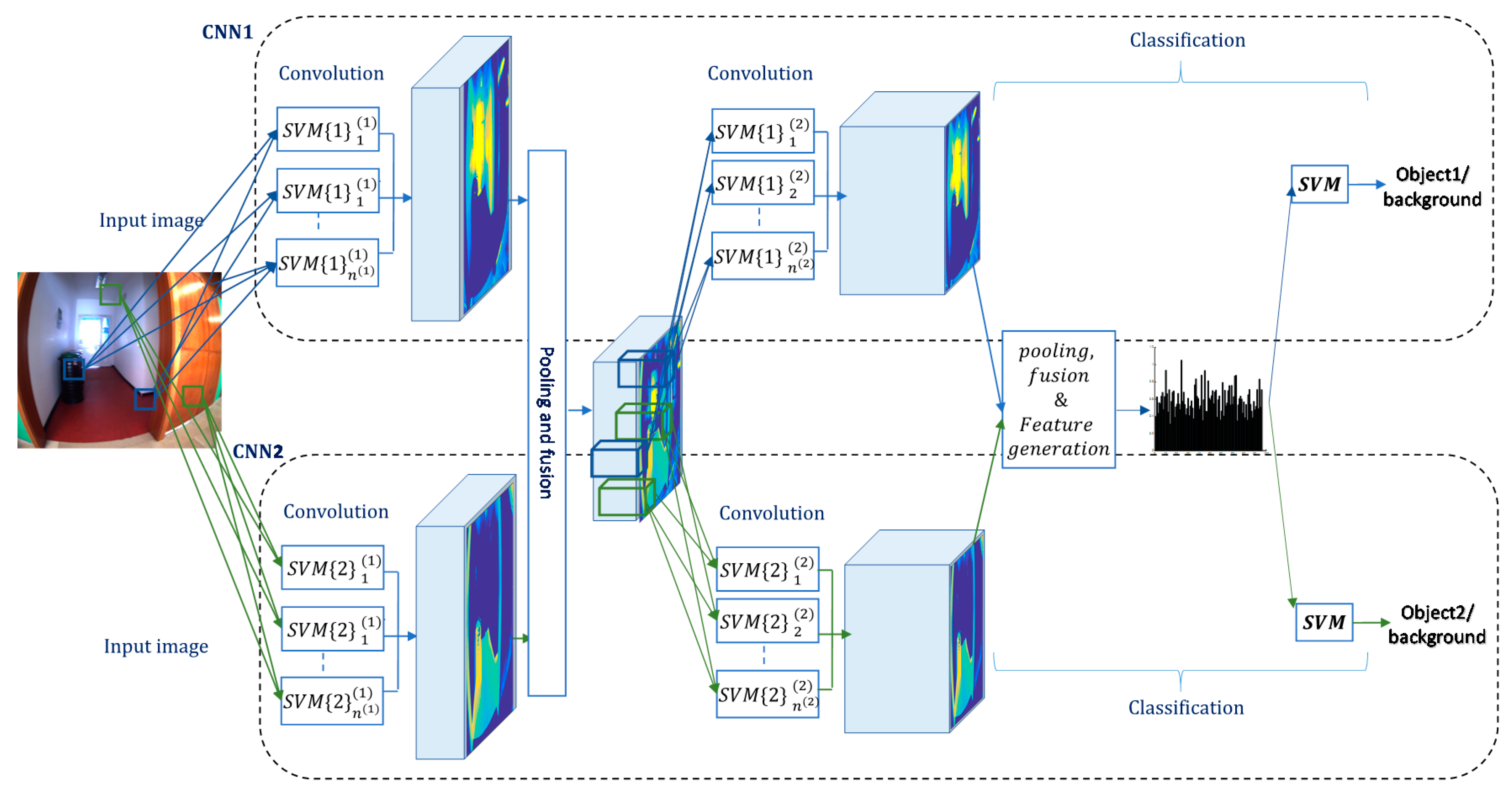
2. Proposed Methodology

Let us consider a set of M training RGB images { X i , y i } i = 1 M of size r × c acquired by a portable digital camera mounted on a lightweight shield worn by the user, and connected via a USB wire to a laptop processing unit, where X i r × c × 3 , and ( r , c) refer the number of rows and columns of the images. Let us assume also y i = [ y 1 , y 2 , , y K ] T is its corresponding label vector, where K represents the total number of targeted classes. In a multi-label setting, the label y i = 1 is set to 1 if the corresponding object is present; otherwise, it is set to 0. Figure 1 shows a general view of the proposed M-CSVM classification system, which is composed from K branches. In next sub-sections, we detail the convolution and fusion layers, which are the main ingredient of the proposed method.

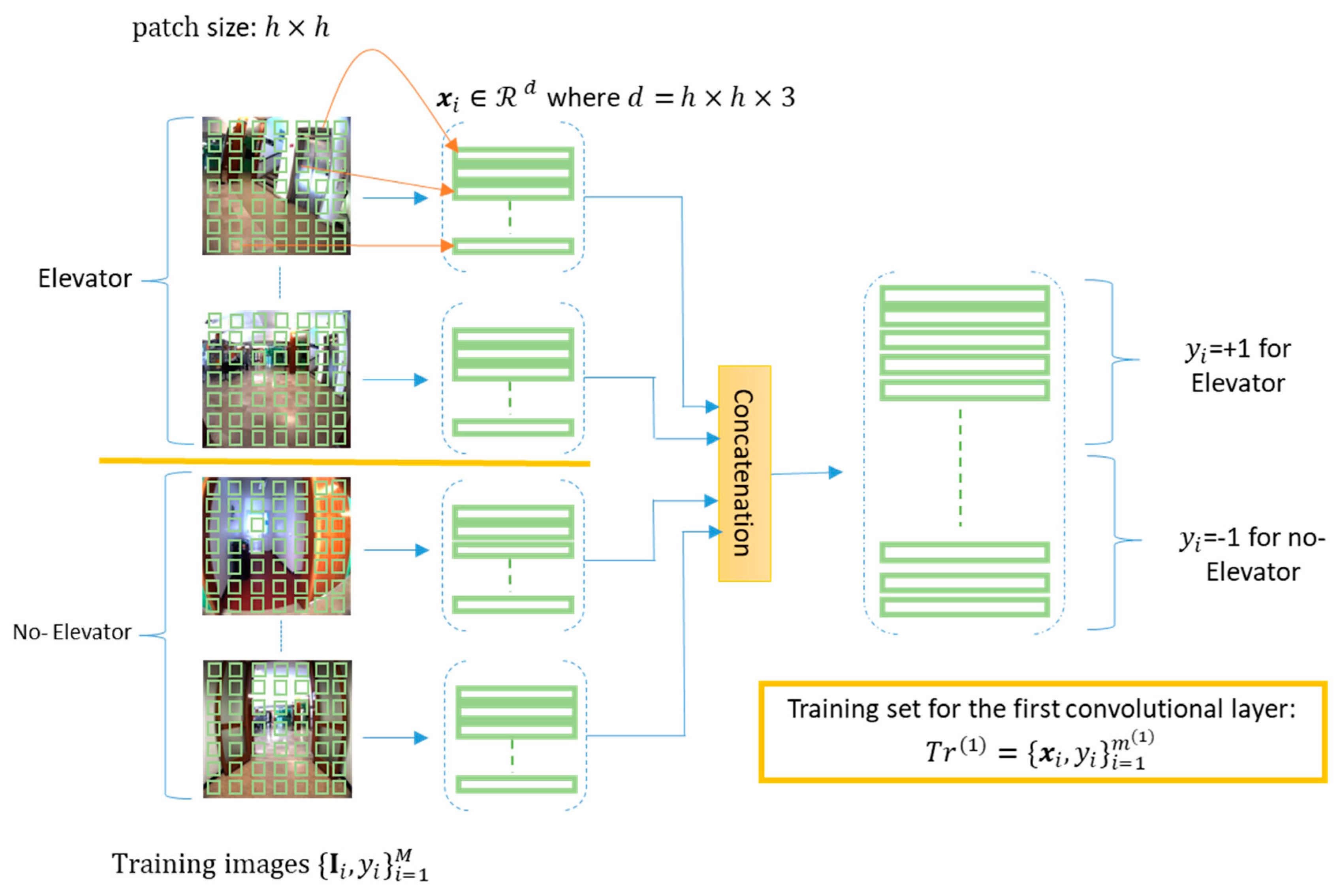
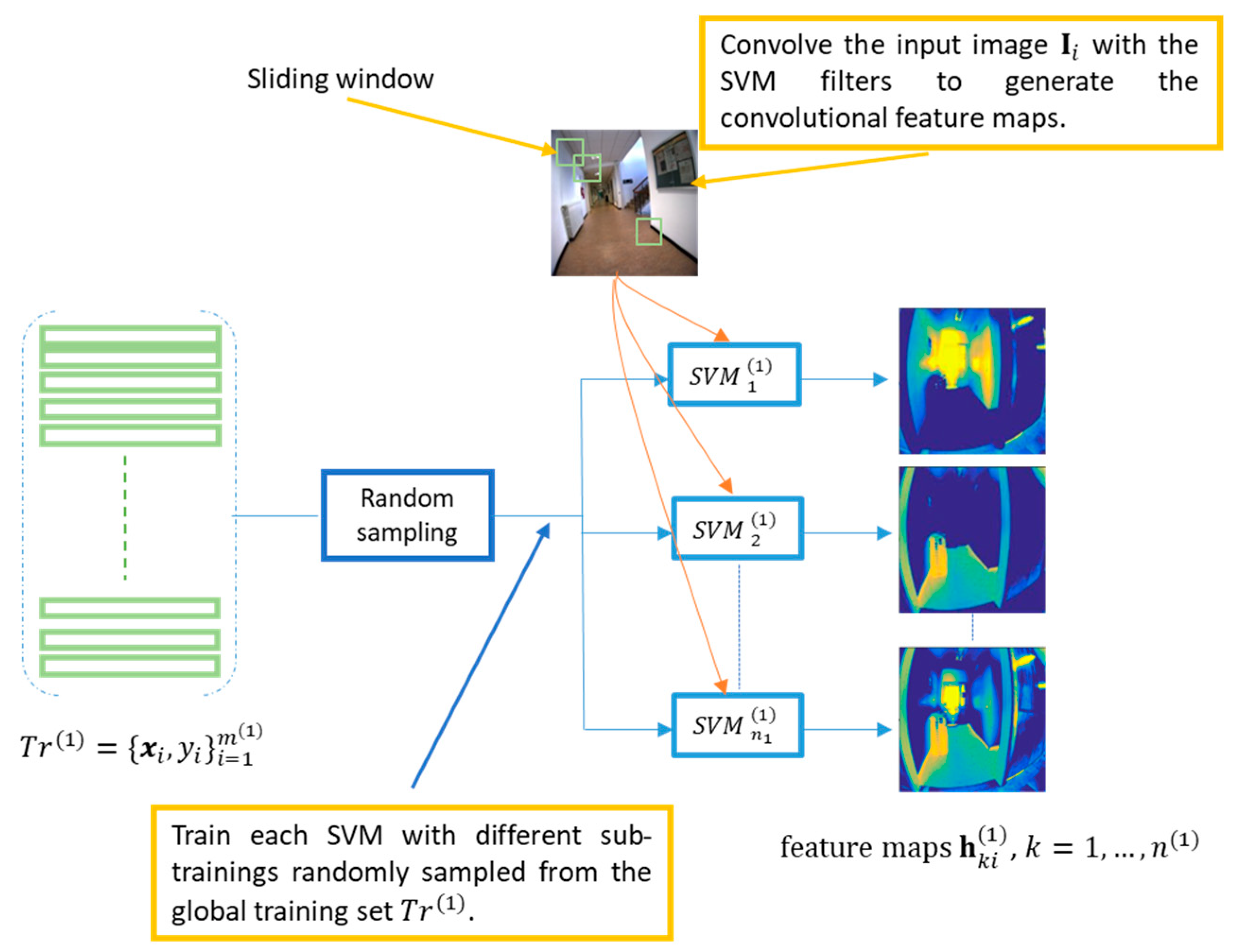
2.1. A. Convolution Layer

In this section, we present the SVM convolution technique for the first convolution layer. The generalization to subsequent layers is straightforward. In a binary classification setting, the training set { X i , y i } i = 1 M is supposed to be composed of M positive and negative RGB images and the corresponding class labels are set to y i { + 1 , 1 } . The positive images contain the object of interest, whereas the negatives ones represent background. From each image X i , we extract a set of patches of size h × h × 3 and represent them as feature vectors x i of dimension d , with d = h × h × 3 . After processing the M training images, we obtain a large training set T r ( 1 ) = { x i , y i } i = 1 m ( 1 ) of size m ( 1 ) as shown in Figure 2.
Next, we learn a set of SVM filters on different sub-training sets T r s u b ( 1 ) = { x i , y i } i = 1 l of size l randomly sampled from the training set T r ( 1 ) . The weight vector w d and bias b of each SVM filter are determined by optimizing the following problem [39,40]:
min w , b w T w + C i = 1 l ξ ( w , b ; x i , y i )
where C is a penalty parameter, which can be estimated through cross-validation. As loss function, we use ξ ( w , b ; x i , y i ) = max ( 1 y i ( w T x i + b ) , 0 ) referred as the hinge loss. After training, we represent the weights of the SVM filters as { w k ( 1 ) } k = 1 n ( 1 ) , where w k ( 1 ) h × h × 3 refers to kth-SVM filter weight matrix, while n ( 1 ) is the number of filters. Then, the complete weights of the first convolution layer are grouped into a filter bank of four dimensions W ( 1 ) h × h × 3 × n ( 1 ) .
In order to generate the feature maps, we simply convolve each training image { X i } i = 1 M , with the obtained filters as is usually done in standard CNN to generate a set of 3D hyper-feature maps { H i ( 1 ) } i = 1 M . Here H i ( 1 ) r ( 1 ) × c ( 1 ) × n ( 1 ) is the new feature representation of image X i composed of n ( 1 ) feature maps (Figure 3). To obtain the kth feature map h k i ( 1 ) , we convolve the kth filter with a set of sliding windows of size h × h × 3 (with a predefined stride) over the training image X i as shown in Figure 4:
h k i ( 1 ) = f ( X i w k ( 1 ) )   ,   k = 1 , ,   n ( 1 )
where is the convolution operator and f is the activation function.
In the following algorithm, we present the implementation of this convolutional layer. The generalization to subsequent convolution layer is simply made by considering the obtained feature maps as new input to the next convolution layer.
Algorithm 1 Convolution layer
Input: Training images { X i , y i } i = 1 M ; SVM filters: n ( 1 ) ; filter parameters (width h , and stride);
    l : size of sampled training set for generating a single feature map.
Output: Feature maps: H ( 1 ) r ( 1 ) × c ( 1 ) × n ( 1 ) × M
1: T r ( 1 ) = global _ training ( { I i , y i } i = 1 M ) ;
2:   W ( 1 ) = learn _ SVM _ filters ( T r ( 1 ) , n ( 1 ) , l )
3: H ( 1 ) = convolution ( { X i } i = 1 M ,   W ( 1 ) ) ;
4: H ( 1 ) = R e L U ( H ( 1 ) )

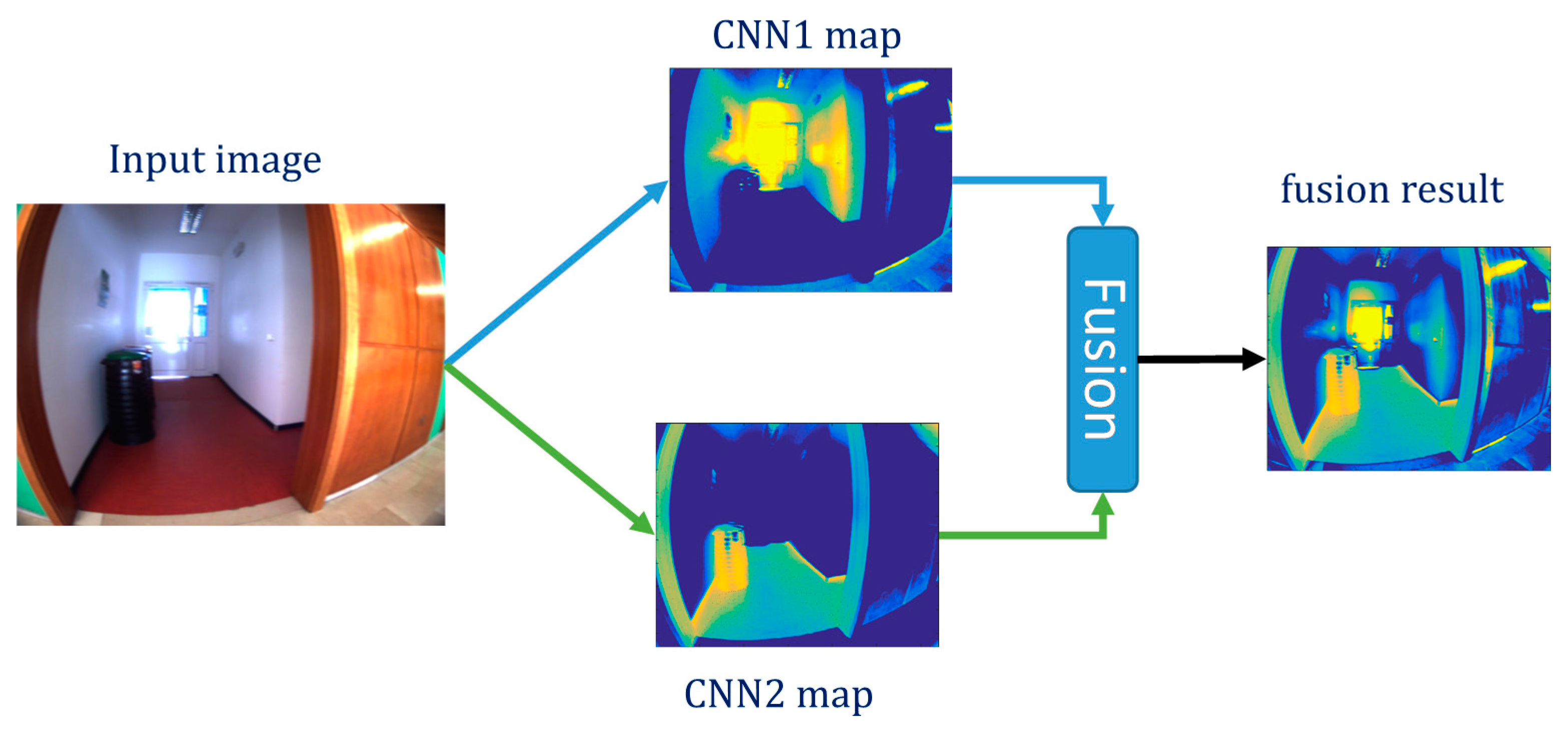
2.2. B. Fusion Layer

In a multi-label setting, we run multiple CSVMs depending on the number of objects. Each CSVM will apply a set of convolutions on the image under analysis as shown in Figure 1. Then each convolution layer is followed by a spatial reduction layer. This reduction layer is similar to the spatial pooling layer in standard CNNs. It is commonly used to reduce the spatial size of the feature maps by selecting the most useful features for the next layers. It takes small blocks from the resulting features maps and sub-samples them to produce a single output from each block. Here, we use the average pooling operator for carrying out reduction. Then, to exploit the correlation between objects present in the image, we propose to fuse the feature maps provided by each branch. In particular, we opt for the max-pooling strategy in order to highlight the different detected objects by each branch. Figure 4 shows an example of fusion process for two branches. The input image contains two objects, Laboratories (object1) and Bins (object2). The first CSVM tries to highlight the first object, while the second one is devoted for the second object. The output maps provided by the pooling operation are fused using the max-rule in order to get a new feature-map where the two concerned objects are highlighted as can be seen in Figure 4. We recall that the feature maps obtained by this operation will be used as input to the next convolution layer for each branch.
Algorithm 2 Pooling and fusion
Input: Feature maps: H ( i ) i = 1,…, K produced by the ith CSVM branch
Output: Fusion result: H ( f 1 )
1: Apply an average pooling to each H ( i ) to generate a set of activation maps of reduced spatial size.
2: Fuse the resulting activation using max rule to generate the feature map H ( f 1 ) . These maps will be used as a common input to the next convolution layers in each CSVM branch.

2.3. C. Feature Generation and Classification

After applying several convolutions, reduction, and fusion layers, the high-level reasoning of the network is done by training K binary SVM classifiers to detect the presence/absence of the objects in the image. If we let { H i ( L ) , y i } i = 1 M be the hyper-feature maps obtained by the last computing layer (convolution or reduction depending on the network architecture) and, if we suppose also that each hyper-feature map H i ( L ) is composed of n ( L ) feature maps, then a possible solution for extracting the high-level feature vector z i n ( L ) of dimension for the training image X i could be simply done by computing the mean or max value for each feature map.

3. Experimental Results

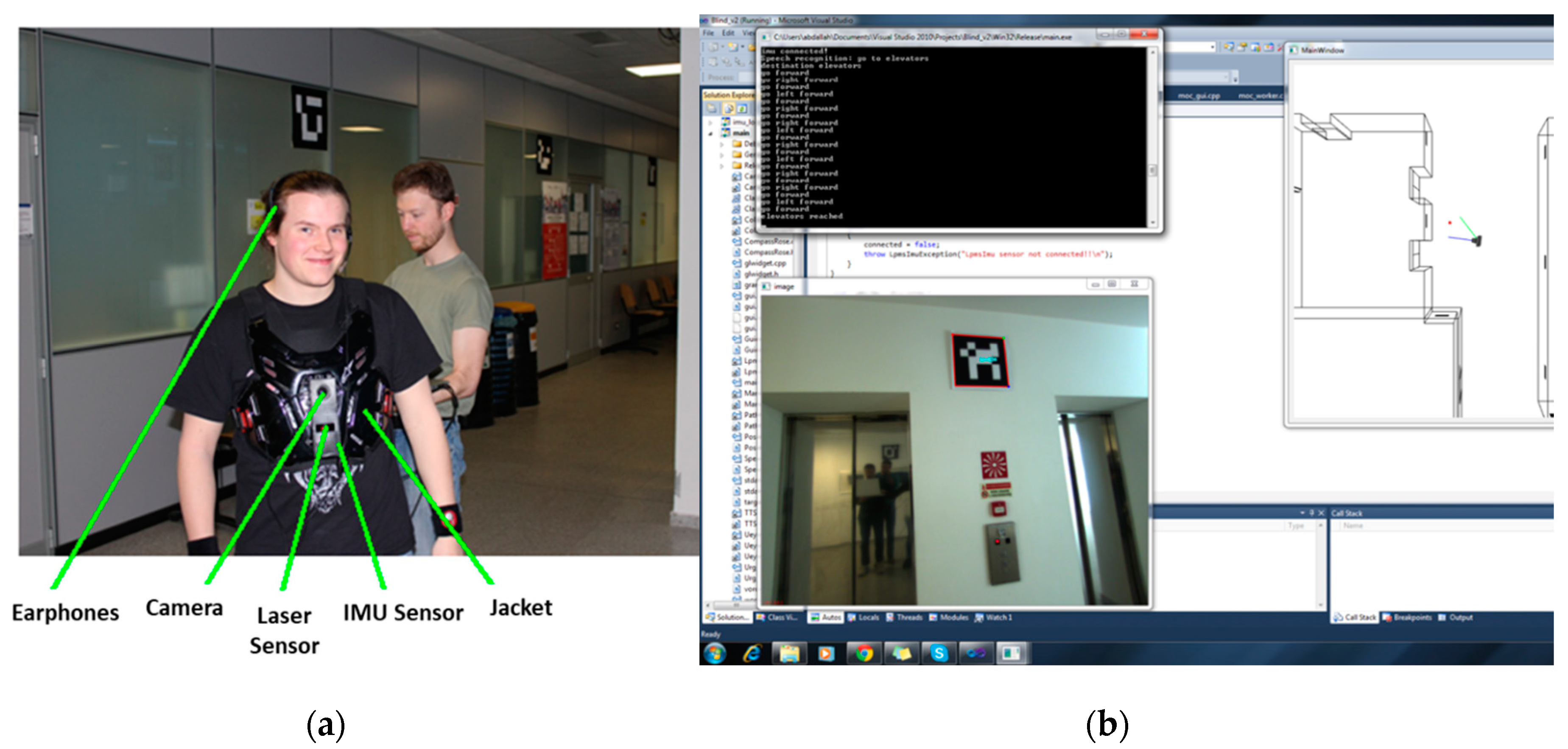
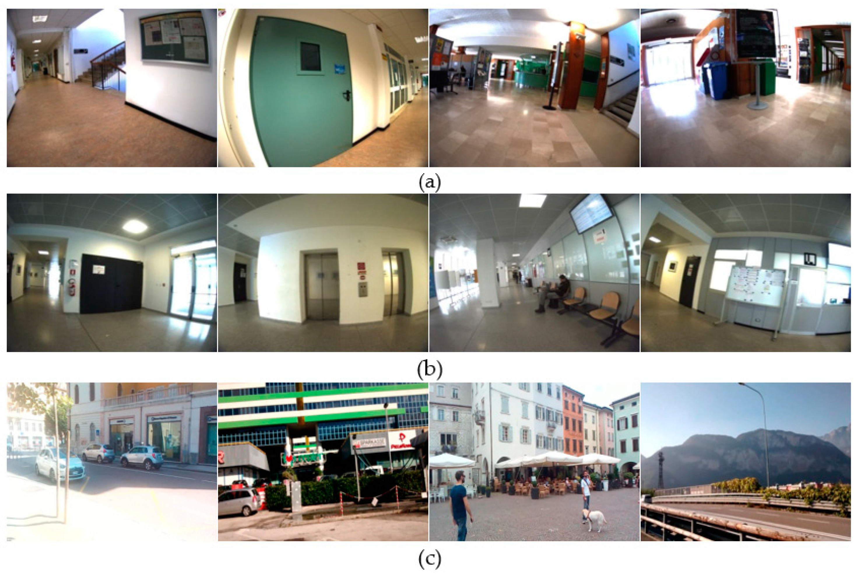
3.1. Dataset Description

In the experiments, we evaluate the proposed method on three datasets taken by a portable camera mounted on a lightweight shield worn by the user, and connected via a USB wire to a laptop processing unit. This system incorporates navigation and recognition modules. In a first step, the user runs the application to load the offline-stored information related to recognition and navigation. Then he can control this system using verbal commands as shown in Figure 5a. For the sake of clarity, we provide also a general view of the application, where the user asks to go to the ‘elevator’. Upon the arrival to the desired destination using a path planning module, the prototype notifies the user that the destination is reached. Figure 5b shows the current view of the camera, where the destination (elevators) is displayed. The system also features a virtual environment emulating the real movement of the user within the indoor space. As can be seen, the user is symbolized by the black top-silhouette, emitting two lines, the blue line refers to the user’s current frontal view; the green point refers to the destination estimated by the path planning module; while the red dot highlights the final destination. The interface displays also markers displayed as thick lines laying on the walls for helping in the localization. In our work, we have used this system to acquire different images used for developing the recognition module based on M-CSVM.
The first and second datasets acquired by this system are composed of images of size 320 × 240 pixels. Both datasets have been taken at two different indoor spaces of the faculty of science of University of Trento (Italy). The first dataset contains 58 training and 72 testing images, whereas the second dataset contains 61 training images and 70 testing images. On the other the side, the third dataset is related to outdoor environment and was acquired over different locations across the city of Trento. The locations were selected based on their importance as well as the density of people frequenting them. The dataset comprises two hundred (200) images of size 275 × 175 pixels, which were equally divided into 100 training and testing images, respectively. It is noteworthy that the training images for all datasets were selected in such a way as to cover all the predefined objects in the considered indoor and outdoor environments. To this end, we have selected the objects deemed to be the most important ones in the considered spaces. Regarding the first dataset, 15 objects were considered as follows: ‘External Window’, ‘Board’, ‘Table’, ‘External Door’, ‘Stair Door’, ‘Access Control Reader’, ‘Office’, ‘Pillar’, ‘Display Screen’, ‘People’, ‘ATM’, ‘Chairs’, ‘Bins’, ‘Internal Door’, and ‘Elevator’. Whereas, for the second set, the list was the following: ‘Stairs’, ‘Heater’, ‘Corridor’, ‘Board’, ‘Laboratories’, ‘Bins’, ‘Office’, ‘People’, ‘Pillar’, ‘Elevator’, ‘Reception’, ‘Chairs’, ‘Self Service’, ‘External Door’, and ‘Display Screen’. Finally, for the last dataset, a total of 26 objects were defined as follows: ‘People’, ‘Building’, ‘Bar(s)’, ‘Monument(s)’, ‘Chairs/Benches’, ‘Green ground’, ‘Vehicle(s)’, ‘Stairs’, ‘Walk path/Sidewalk’, ‘Fence/Wall’, ‘Tree(s)/Plant(s)’, ‘Garbage can(s)’, ‘Bus stop’, ‘Crosswalk’, ‘River’, ‘Roundabout’, ‘Pole(s)/Pillar(s)’, ‘Shop(s)’, ‘Supermarket(s)’, ‘Pound/Birds’, ‘Underpass’, ‘Bridge’, ‘Railroad’, ‘Admiration building’, ‘Church’, and ‘Traffic signs’. Figure 6 shows sample images from each dataset.
In the experiments, we assessed the performances of the method in terms of sensitivity (SEN) and specificity (SPE) measures:
SEN = True   Positive True   Positive + False   Negative
SPE = True   Negative True   Negative + False   Positive
The sensitivity expresses the classification rate of real positive cases, i.e., the efficiency of the algorithm towards detecting existing objects. The specificity, on the other hand, underlines the tendency of the algorithm to detect the true negatives, i.e., the non-existing objects. We also propose to compute the average of the two earlier measures as follows:
AVG = SEN + SPE 2

3.2. Results

The architecture of the proposed CSVM involves many parameters. To identify a suitable architecture, we propose to investigate three main parameters, which are: the number of layers of the network, number of feature maps generated by each convolution layer and the spatial sizes of the kernels. To compute the best parameter values, we use a cross-validation technique with a number of folds equal to 3. Due to the limited number of training samples and the large number of possible combinations, we set the maximum number of possible layers to 3, the maximum number of SVMs in each layer to 512 with step of 2 i (i = 0,…,9) and maximum kernel size for each layer is fixed to 10% of the size of the current map (we consider the minimum between the height and the width as the considered size) with step of 2. The obtained best values of the parameters by cross-validation are listed in Table 1. This table indicates that only one layer is enough for the first dataset, whereas the two other datasets require two layers to get the best performances. Concerning the number of SVMs and the related spatial size, dataset 3 presents the simplest architecture with just one SVM at the first layer and two SVMs at the second one with spatial size of 3. It is worth recalling that in the experiments.
In order to evaluate our method, we compare it with results obtained using three different pre-trained CNNs, which are ResNet [23], GoogLeNet [24] and VGG16 [33]. All the results in terms of accuracies are reported in Table 2.
From these tables, it can be seen that in eight cases out of nine, our proposed method by far outperforms the different pre-trained CNNs. In seven cases the improvement is clearly important (more than 2%). Only in one case (ResNet, dataset 2) does a CNN method give a slightly better result than our method (92.96% compared to 92.90%).

4. Discussion

Besides the classification accuracies, another important performance parameter is the runtime. Table 3 shows the training time of the proposed method for the three datasets. It can be seen clearly that the training of M-CSVM is fast and needs just few seconds to few minutes in the worse case. In details, dataset 1 presents the highest runtime (76 s) which is due to the high number of filters used for this dataset (512), while training of dataset 3 is much faster (just 8 s) due to the simplicity of the related network (see Table 1).
Regarding runtime at the prediction phase, which includes the feature extraction and classification, the M-CSVM method presents different runtime for the three datasets depending on the complexity of the adopted architecture. For instance, as we can see in Table 4, the highest runtime is with the first dataset 1 with 0.200 s per image, which is due to the high number of filters adopted for it (512). In contrast, the third dataset requires only 0.002 s to extract features and estimate the classes for each image. This short time is due to the small number of SVMs used in this network for this dataset. It is also important to mention that the runtime provided by our method outperforms the three pre-trained CNNs on two datasets (datasets 2 and 3), especially for the dataset 3 where the difference is significant. Except for dataset 1, where GoogLeNet is slightly faster due to complexity of the related network.

5. Conclusions

In this paper, we have presented a novel M-CSVM method for describing the image content for VI people. This method has the following important proprieties: (1) it allows SVMs to act as convolutional filters; (2) it uses a forward supervised learning strategy for computing the weights of the filters; and (3) it estimates each layer locally, which reduces the complexity of the network. The experimental results obtained on the three datasets with limited training samples confirm the promising capability of the proposed method with respect to state-of-the-art methods based on pre-trained CNNs. For future developments, we plan to investigate architectures based on residual connections such as in modern networks, and to explore uses of advanced strategies based on reinforcement learning for finding an optimized M-CVSM architecture. Additionally, we plan to extend this method to act as a detector by localizing the detected object in the image.

Author Contributions

Y.B. implemented the method and wrote the paper. H.A., N.A., and F.M. contributed to the analysis of the experimental results and paper writing.

Funding

This work was supported by NSTIP Strategic Technologies Programs, number 13-MED-1343-02 in the Kingdom of Saudi Arabia.

Acknowledgments

This work was supported by NSTIP Strategic Technologies Programs number: 13-MED-1343-02 in the Kingdom of Saudi Arabia.

Conflicts of Interest

The authors declare no conflict of interest.

References

  1. Blindness and Vision Impairment. Available online: https://www.who.int/news-room/fact-sheets/detail/blindness-and-visual-impairment (accessed on 12 September 2019).
  2. Ulrich, I.; Borenstein, J. The GuideCane-applying mobile robot technologies to assist the visually impaired. IEEE Trans. Syst. Man Cybern. Part A Syst. Hum. 2001, 31, 131–136. [Google Scholar] [CrossRef]
  3. Shoval, S.; Borenstein, J.; Koren, Y. The NavBelt-a computerized travel aid for the blind based on mobile robotics technology. IEEE Trans. Biomed. Eng. 1998, 45, 1376–1386. [Google Scholar] [CrossRef]
  4. Bahadir, S.K.; Koncar, V.; Kalaoglu, F. Wearable obstacle detection system fully integrated to textile structures for visually impaired people. Sens. Actuators A Phys. 2012, 179, 297–311. [Google Scholar] [CrossRef]
  5. Shin, B.-S.; Lim, C.-S. Obstacle Detection and Avoidance System for Visually Impaired People. In Proceedings of the Haptic and Audio Interaction Design, Seoul, Korea, 29–30 November 2007; Oakley, I., Brewster, S., Eds.; Springer: Berlin/Heidelberg, Germany, 2007; pp. 78–85. [Google Scholar]
  6. Bousbia-Salah, M.; Bettayeb, M.; Larbi, A. A Navigation Aid for Blind People. J. Intell. Robot. Syst. 2011, 64, 387–400. [Google Scholar] [CrossRef]
  7. Brilhault, A.; Kammoun, S.; Gutierrez, O.; Truillet, P.; Jouffrais, C. Fusion of Artificial Vision and GPS to Improve Blind Pedestrian Positioning. In Proceedings of the 2011 4th IFIP International Conference on New Technologies, Mobility and Security, Paris, France, 7–10 February 2011; pp. 1–5. [Google Scholar]
  8. Hasanuzzaman, F.M.; Yang, X.; Tian, Y. Robust and Effective Component-Based Banknote Recognition for the Blind. IEEE Trans. Syst. Man Cybern. Part C (Appl. Rev.) 2012, 42, 1021–1030. [Google Scholar] [CrossRef]
  9. López-de-Ipiña, D.; Lorido, T.; López, U. BlindShopping: Enabling Accessible Shopping for Visually Impaired People through Mobile Technologies. In Proceedings of the Toward Useful Services for Elderly and People with Disabilities, Montreal, QC, Canada, 20–22 June 2011; Abdulrazak, B., Giroux, S., Bouchard, B., Pigot, H., Mokhtari, M., Eds.; Springer: Berlin/Heidelberg, Germany, 2011; pp. 266–270. [Google Scholar]
  10. Tekin, E.; Coughlan, J.M. An Algorithm Enabling Blind Users to Find and Read Barcodes. Proc. IEEE Workshop Appl. Comput. Vis. 2009, 2009, 1–8. [Google Scholar]
  11. Pan, H.; Yi, C.; Tian, Y. A primary travelling assistant system of bus detection and recognition for visually impaired people. In Proceedings of the 2013 IEEE International Conference on Multimedia and Expo Workshops (ICMEW), San Jose, CA, USA, 15–19 July 2013; pp. 1–6. [Google Scholar]
  12. Jia, T.; Tang, J.; Lik, W.; Lui, D.; Li, W.H. Plane-based detection of staircases using inverse depth. In Proceedings of the Australasian Conference on Robotics and Automation (ACRA), Wellington, New Zealand, 3–5 December 2012. [Google Scholar]
  13. Chen, X.R.; Yuille, A.L. Detecting and reading text in natural scenes. In Proceedings of the 2004 IEEE Computer Society Conference on Computer Vision and Pattern Recognition (CVPR), Washington, DC, USA, 27 June–2 July 2004; Volume 2, p. II. [Google Scholar]
  14. Yang, X.; Tian, Y. Robust door detection in unfamiliar environments by combining edge and corner features. In Proceedings of the 2010 IEEE Computer Society Conference on Computer Vision and Pattern Recognition-Workshops, San Francisco, CA, USA, 13–18 June 2010; pp. 57–64. [Google Scholar]
  15. Wang, S.; Tian, Y. Camera-Based Signage Detection and Recognition for Blind Persons. In Proceedings of the Computers Helping People with Special Needs, Linz, Austria, 11–13 July 2012; Miesenberger, K., Karshmer, A., Penaz, P., Zagler, W., Eds.; Springer: Berlin/Heidelberg, Germany, 2012; pp. 17–24. [Google Scholar]
  16. Fernandes, H.; Costa, P.; Paredes, H.; Filipe, V.; Barroso, J. Integrating Computer Vision Object Recognition with Location Based Services for the Blind. In Proceedings of the Universal Access in Human-Computer Interaction. Aging and Assistive Environments, Heraklion, Greece, 22–27 June 2014; Stephanidis, C., Antona, M., Eds.; Springer International Publishing: Cham, Switzerland, 2014; pp. 493–500. [Google Scholar]
  17. Tian, Y.; Yang, X.; Yi, C.; Arditi, A. Toward a computer vision-based wayfinding aid for blind persons to access unfamiliar indoor environments. Mach. Vis. Appl. 2013, 24, 521–535. [Google Scholar] [CrossRef]
  18. Malek, S.; Melgani, F.; Mekhalfi, M.L.; Bazi, Y. Real-Time Indoor Scene Description for the Visually Impaired Using Autoencoder Fusion Strategies with Visible Cameras. Sensors 2017, 17, 2641. [Google Scholar] [CrossRef]
  19. Mekhalfi, M.L.; Melgani, F.; Bazi, Y.; Alajlan, N. Fast indoor scene description for blind people with multiresolution random projections. J. Vis. Commun. Image Represent. 2017, 44, 95–105. [Google Scholar] [CrossRef]
  20. Moranduzzo, T.; Mekhalfi, M.L.; Melgani, F. LBP-based multiclass classification method for UAV imagery. In Proceedings of the 2015 IEEE International Geoscience and Remote Sensing Symposium (IGARSS), Milan, Italy, 26–31 July 2015; pp. 2362–2365. [Google Scholar]
  21. Mariolis, I.; Peleka, G.; Kargakos, A.; Malassiotis, S. Pose and category recognition of highly deformable objects using deep learning. In Proceedings of the 2015 International Conference on Advanced Robotics (ICAR), Istanbul, Turkey, 27–31 July 2015; pp. 655–662. [Google Scholar]
  22. He, K.; Zhang, X.; Ren, S.; Sun, J. Spatial Pyramid Pooling in Deep Convolutional Networks for Visual Recognition. In Proceedings of the Computer Vision–ECCV 2014, Zurich, Switzerland, 6–12 September 2014; Springer: Cham, Switzerland, 2014; pp. 346–361. [Google Scholar]
  23. He, K.; Zhang, X.; Ren, S.; Sun, J. Deep Residual Learning for Image Recognition. In Proceedings of the 2016 IEEE Conference on Computer Vision and Pattern Recognition (CVPR), Las Vegas, NV, USA, 27–30 June 2016; pp. 770–778. [Google Scholar]
  24. Szegedy, C.; Liu, W.; Jia, Y.; Sermanet, P.; Reed, S.; Anguelov, D.; Erhan, D.; Vanhoucke, V.; Rabinovich, A. Going deeper with convolutions. In Proceedings of the 2015 IEEE Conference on Computer Vision and Pattern Recognition (CVPR), Boston, MA, USA, 7–12 June 2015; pp. 1–9. [Google Scholar]
  25. Krizhevsky, A.; Sutskever, I.; Hinton, G.E. ImageNet Classification with Deep Convolutional Neural Networks. In Proceedings of the 25th International Conference on Neural Information Processing Systems-Volume 1, Lake Tahoe, Nevada, 3–6 December 2012; Curran Associates Inc.: Brooklyn, NY, USA, 2012; pp. 1097–1105. [Google Scholar]
  26. Ren, S.; He, K.; Girshick, R.; Zhang, X.; Sun, J. Object Detection Networks on Convolutional Feature Maps. IEEE Trans. Pattern Anal. Mach. Intell. 2017, 39, 1476–1481. [Google Scholar] [CrossRef] [PubMed]
  27. Girshick, R.; Donahue, J.; Darrell, T.; Malik, J. Region-Based Convolutional Networks for Accurate Object Detection and Segmentation. IEEE Trans. Pattern Anal. Mach. Intell. 2016, 38, 142–158. [Google Scholar] [CrossRef] [PubMed]
  28. Ren, S.; He, K.; Girshick, R.; Sun, J. Faster R-CNN: Towards Real-Time Object Detection with Region Proposal Networks. IEEE Trans. Pattern Anal. Mach. Intell. 2017, 39, 1137–1149. [Google Scholar] [CrossRef] [PubMed]
  29. Ouyang, W.; Zeng, X.; Wang, X.; Qiu, S.; Luo, P.; Tian, Y.; Li, H.; Yang, S.; Wang, Z.; Li, H.; et al. DeepID-Net: Object Detection with Deformable Part Based Convolutional Neural Networks. IEEE Trans. Pattern Anal. Mach. Intell. 2017, 39, 1320–1334. [Google Scholar] [CrossRef] [PubMed]
  30. Farabet, C.; Couprie, C.; Najman, L.; LeCun, Y. Learning Hierarchical Features for Scene Labeling. IEEE Trans. Pattern Anal. Mach. Intell. 2013, 35, 1915–1929. [Google Scholar] [CrossRef] [PubMed]
  31. Sun, W.; Wang, R. Fully Convolutional Networks for Semantic Segmentation of Very High Resolution Remotely Sensed Images Combined With DSM. IEEE Geosci. Remote Sens. Lett. 2018, 15, 474–478. [Google Scholar] [CrossRef]
  32. Srivastava, N.; Hinton, G.; Krizhevsky, A.; Sutskever, I.; Salakhutdinov, R. Dropout: A Simple Way to Prevent Neural Networks from Overfitting. J. Mach. Learn. Res. 2014, 15, 1929–1958. [Google Scholar]
  33. Simonyan, K.; Zisserman, A. Very Deep Convolutional Networks for Large-Scale Image Recognition. arXiv 2014, arXiv:1409.1556. [Google Scholar]
  34. Chatfield, K.; Simonyan, K.; Vedaldi, A.; Zisserman, A. Return of the Devil in the Details: Delving Deep into Convolutional Nets. arXiv 2014, arXiv:1405.3531. [Google Scholar]
  35. Azizpour, H.; Razavian, A.S.; Sullivan, J.; Maki, A.; Carlsson, S. Factors of Transferability for a Generic ConvNet Representation. IEEE Trans. Pattern Anal. Mach. Intell. 2016, 38, 1790–1802. [Google Scholar] [CrossRef]
  36. Nogueira, R.F.; de Alencar Lotufo, R.; Machado, R.C. Fingerprint Liveness Detection Using Convolutional Neural Networks. IEEE Trans. Inf. Forensics Secur. 2016, 11, 1206–1213. [Google Scholar] [CrossRef]
  37. Gao, C.; Li, P.; Zhang, Y.; Liu, J.; Wang, L. People counting based on head detection combining Adaboost and CNN in crowded surveillance environment. Neurocomputing 2016, 208, 108–116. [Google Scholar] [CrossRef]
  38. Bazi, Y.; Melgani, F. Convolutional SVM Networks for Object Detection in UAV Imagery. IEEE Trans. Geosci. Remote Sens. 2018, 56, 3107–3118. [Google Scholar] [CrossRef]
  39. Fan, R.-E.; Chang, K.-W.; Hsieh, C.-J.; Wang, X.-R.; Lin, C.-J. Liblinear: A Library for Large Linear Classification. J. Mach. Learn. Res. 2008, 9, 1871–1874. [Google Scholar]
  40. Chang, K.; Lin, C. Coordinate Descent Method for Large-scale L2-loss Linear Support Vector Machines. J. Mach. Learn. Res. 2008, 9, 1369–1398. [Google Scholar]
Figure 1. Proposed multi-label convolutional support vector machine (M-CSVM) architecture for detecting the presence of multiple objects in the image.
Applsci 09 05062 g001
Figure 2. Training set generation for the first convolution layer.
Applsci 09 05062 g002
Figure 3. Supervised feature map generation.
Applsci 09 05062 g003
Figure 4. Example of fusion of output maps of two convolutional neural networks (CNNs).
Applsci 09 05062 g004
Figure 5. Overview of the system developed for visually impaired (VI) people. (a) Camera mounted on the chest, tablet, and headphones for voice communication; and (b) graphical interface.
Applsci 09 05062 g005
Figure 6. Example of images taken by a portable camera: (a) dataset 1, (b) dataset 2, and (c) dataset 3.
Applsci 09 05062 g006
Table 1. Best parameter values of the convolutional support vector machine (CSVM) for each dataset.
DatasetLayer 1Layer 2
Number of SVMsSpatial SizeNumber of SVMsSpatial Size
Dataset 15127//
Dataset 23272563
Dataset 31323
Table 2. Classification obtained by M-CSVM compared to CNNs for: (a) dataset 1, (b) dataset 2, and (c) dataset 3.
(a)
MethodSEN (%)SPE (%)AVG (%)
ResNet71.1693.8482.50
GoogLeNet78.6594.3486.49
VGG1674.5394.5884.55
Ours89.1484.2686.70
(b)
MethodsSEN (%)SPE (%)AVG (%)
ResNet89.5496.3892.96
GoogLeNet83.6396.8690.25
VGG1681.8196.1488.98
Ours93.6492.1792.90
(c)
MethodsSEN (%)SPE (%)AVG (%)
ResNet64.1792.4078.29
GoogLeNet62.5093.2777.88
VGG1664.3293.9879.15
Ours80.7982.2781.53
Table 3. Training time of the proposed M-CSVM.
DatasetRuntime (s)
Dataset 176
Dataset 242
Dataset 38
Table 4. Comparison of average runtime per image for: (a) dataset 1, (b) dataset 2, and (c) dataset 3.
(a)
MethodRuntime (s)
ResNet0.207
GoogLeNet0.141
VGG160.291
Ours0.206
(b)
MethodRuntime (s)
ResNet0.208
GoogLeNet0.144
VGG160.291
Ours0.115
(c)
MethodRuntime (s)
ResNet0.207
GoogLeNet0.145
VGG160.300
Ours0.002

