Precise Photon Correlation Measurement of a Chaotic Laser

Featured Application

This technique of improving the accuracy of g⁽²⁾(τ) measurement is useful to extract higher order coherence and achieve desired laser source for quantum imaging and secure communication.

Abstract

The second order photon correlation g⁽²⁾(τ) of a chaotic optical-feedback semiconductor laser is precisely measured using a Hanbury Brown–Twiss interferometer. The accurate g⁽²⁾(τ) with non-zero delay time is obtained experimentally from the photon pair time interval distribution through a ninth-order self-convolution correction. The experimental results agree well with the theoretical analysis. The relative error of g⁽²⁾(τ) is no more than 5‰ within 50 ns delay time. The bunching effect and coherence time of the chaotic laser are measured via the precise photon correlation technique. This technique provides a new tool to improve the accuracy of g⁽²⁾(τ) measurement and boost applications of quantum statistics and correlation.

1. Introduction

Semiconductor lasers subject to external optical feedback exhibit a rich variety of nonlinear dynamical behaviors and are used to generate high-dimensional chaotic lasers [1,2]. This configuration has attracted great interest for a wide range of applications, like optical chaos communication [3,4,5,6,7], secure key distribution [8], high-speed physical random number generation [9,10,11,12], chaos-based optical computing [13] and sensing [14,15,16]. It is fundamentally important to understand the underlying physical mechanisms of the chaotic laser, and practically useful to improve the laser performance and motivate its applications. Previous research mainly focused on clarifying intensity statistics and autocorrelation (AC) of chaotic lasers to characterize chaotic processes [17,18,19,20,21]. Intensity statistics are closely relevant to the extractable rate of random numbers [9,10,22] and the AC is a good indicator of a chaotic modulating bandwidth in optical chaos communications [4,19]. However, the macro-scale intensity statistics and AC are not sufficient to reveal all properties of a given chaotic laser, and there is also a significant discrepancy between experimental and theoretical probability density distributions of the laser intensity [19]. Recent research reveals that quantum correlation is more accurate in assessing statistical properties and more sensitive to control parameters compared to the AC function [23,24]. However, the previous research is concentrated on the properties of the quantum dot laser in the low-intensity (low-gain) situation, and the bunching effect of the chaotic laser, i.e., g⁽²⁾(0) > 1 at τ = 0, is only revealed in the fully developed chaotic (high-gain) regime. Studies on high order photon correlation of high-dimensional chaotic lasers are sparse, especially second order photon correlation g⁽²⁾(τ) at non-zero delay time.

The landmark experiment on photon correlation was first conducted by Hanbury Brown and Twiss (HBT), demonstrating spatial second order photon correlation g⁽²⁾ of a thermal light [25]. Soon afterwards, this experiment inspired Glauber’s seminal work on quantum optics theory, which described the photon correlation of different light fields by correlation functions of quantum statistics [26,27,28]. The photon correlation g⁽²⁾ is fundamentally different from the first order correlation and is harnessed in many applications, such as photon bunching and anti-bunching measurement [29,30,31,32], spatial interference [33,34], ghost imaging [35,36,37], the azimuthal HBT effect [38], single photon detection [39], etc. The g⁽²⁾(τ) also carries a wealth of information on the statistical probability of different photons arriving at time delay τ [40]. Up until now, there are many approaches to obtain photon correlation g⁽²⁾(τ), typically including two-photon absorption (TPA) measurement [41,42], photon coincidence counting [43], time interval measurement of photon pairs [44]. Recently, the HBT experiment was explored to observe chaos from quantum dot lasers with external feedback [23]. However, research on photon correlation g⁽²⁾(τ) of high-dimensional chaotic waveforms is rare and there is still an obvious disagreement between experimental and theoretical g⁽²⁾(τ). The calculation of g⁽²⁾(τ) from the photon pair time interval distribution provides a good way to measure the photon correlation of pseudo-thermal light with microsecond coherence time [44]. But for a chaotic laser, the coherence time is much shorter than that of pseudo-thermal light, and the resolution time must be shorter than the coherence time of the laser in the measurement. Although the shorter coherence time does not affect the bunching effect or g⁽²⁾(0) of the chaotic laser [24], that makes the measurement of g⁽²⁾(τ) (τ ≠ 0) at very short timescales using the HBT technique more difficult, owing to the limited response time of single-photon detectors [45]. It remains an important challenge to ravel the g⁽²⁾(τ) (τ ≠ 0) of the chaotic laser at high precision, whose coherence time is below 1 ns. Accordingly, high precision and ultrashort resolution time are required to acquire an accurate g⁽²⁾(τ) of the chaotic laser. That is, it is potentially useful to extract higher order coherence and achieve a desired laser source for quantum imaging and secure communication.

In this paper, we theoretically and experimentally investigate the second order photon correlation g⁽²⁾(τ) of a chaotic optical-feedback semiconductor laser. The g⁽²⁾(τ) is precisely measured using self-convolution HBT detection at tens of picoseconds resolution time. A different high order correction of g⁽²⁾(τ) is analyzed and confirmed experimentally, which has a low relative error in wide range of delay time. It shows a good agreement between experimental results and theoretical analysis. We also measure the bunching effect and coherence time of the chaotic laser using the precise photon correlation technique. This technique, avoiding the photon overlapping, can give a g⁽²⁾(τ) with a high accuracy. To the best of our knowledge, the accurate measurement of g⁽²⁾(τ) for the chaotic laser has not been investigated and reported. In view of this demonstration, we present first some highlights of precise photon correlation measurement that are necessary for a better understanding of quantum statistics of the chaotic laser. The demonstration well reveals photon correlation g⁽²⁾(τ) of the chaotic laser and provide a way of studying chaos with quantum optics technique.

2. High Order Correction of g⁽²⁾(τ)

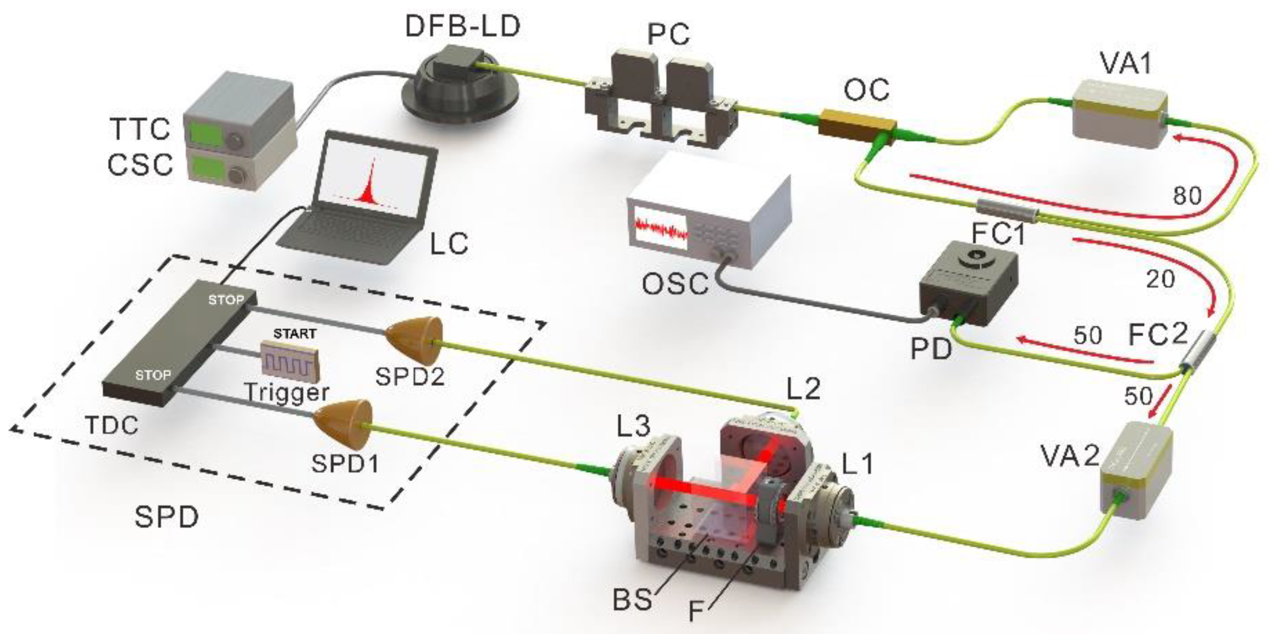
Theoretically, second order photon correlation of g⁽²⁾(τ) can be obtained from an ideal photon pair time interval distribution P₁(τ). Using the self-convolution method, one can obtain any desired high order n, and the higher n of $g_n^{\left(2\right)}$(τ) is, the more accurate $g_n^{\left(2\right)}$(τ) tends to the ideal g⁽²⁾(τ). But due to the actual operation capacity of data processing and the difficulty of convolving complex form to very high order, we reasonably convolve $g_n^{\left(2\right)}$(τ) to the ninth order so the relative error is small enough to obtain high accuracy.

In our experiment, photon pair time interval distribution is collected by single photon counters and the time distribution is D₁(τ). Furthermore, g⁽²⁾(τ) can be calculated from the self-convolution of D₁(τ).

The second order photon correlation g⁽²⁾(τ) has a proportional relation to G(τ), as follows:

$$G(\tau )=\overline{I}{g}^{(2)}(\tau ),$$

(1)

where $\overline{I}$ is the average photon counting rate per time bin of the light field. G(τ) is the histogram of photons at delay time τ between two photon detection events. The relation between G(τ) and P₁(τ) is given by:

$$G(\tau )=P_1(\tau )+P_1(\tau )\ast P_1(\tau )+\dots \dots ={\displaystyle \sum _{n=1}^{\infty }{P}_n(\tau )},$$

(2)

where P₁(τ) is an ideal photon pair time interval distribution of light field which can be obtained based on HBT experiment, and P_n(τ) is nth order self-convolution of P₁(τ). When P₁(τ) is less than one, the sum of P_n(τ) is convergence [40], then we can obtain:

$$P_1(\tau )=L^{-1}(\frac{L(G(\tau ))}{1+L(G(\tau ))}),$$

(3)

where L denotes the Laplace transformation, and L⁻¹ denotes the inverse Laplace transformation.

When the above theory is applied to a Lorentzian chaotic laser field, we can get the relation between G(τ) and P_n(τ) of a chaotic laser. The first order correlation of a Lorentzian chaotic laser is as follows:

$$g^{(1)}(\tau )=e^{-\frac{\left|\tau \right|}{{\tau }_c}}.$$

(4)

The relation between g⁽²⁾(τ) and g⁽¹⁾(τ) for a Lorentzian chaotic laser is:

$$g^{(2)}(\tau )=1+{\left|g^{(1)}(\tau )\right|}^2.$$

(5)

Using Equations (4) and (5), we obtain:

$$g^{(2)}(\tau )=1+{\left|e^{-\left|\tau \right|/{\tau }_c}\right|}^2.$$

(6)

According to Equations (1) and (6), we obtain:

$$G(\tau )=\overline{I}(1+{\left|e^{-\left|\tau \right|/{\tau }_c}\right|}^2).$$

(7)

The relation between g⁽²⁾(τ) and P_n(τ) is shown as follows.

P₂(τ) is the self-convolution of P₁(τ):

$$P_2(\tau )={\displaystyle {\int }_0^{+\infty }{P}_1(\tau )}{P}_1(t-\tau )dt=P_1(\tau )\ast P_1(\tau ).$$

(8)

P₃(τ) is the convolution of P₁(τ) and P₂(τ):

$$P_3(\tau )={\displaystyle {\int }_0^{+\infty }{P}_2(\tau )}{P}_1(t-\tau )dt=P_2(\tau )\ast P_1(\tau ).$$

(9)

P_n(τ) is the convolution of P₁(τ) and P_n−1(τ):

$$P_n(\tau )={\displaystyle {\int }_0^{+\infty }{P}_{n-1}(\tau )}{P}_1(t-\tau )dt=P_{n-1}(\tau )\ast P_1(\tau ).$$

(10)

The integration upper bound of Equation (10) should be replaced by the maximum time interval τ practically. Now the new equation is:

$$P_n(\tau )={\displaystyle {\int }_0^{\tau }{P}_{n-1}(\tau -t)}{P}_1(\tau )dt=P_{n-1}(\tau )\ast P_1(\tau ).$$

(11)

Using Equations (3), (8), (9), (10), and (11), we obtain all of the self-convolution of P₁(τ)

Then we obtain the following equations:

$$P_2(\tau )=L^{-1}(\frac{L(G(\tau ))}{1+L(G(\tau ))})\ast L^{-1}(\frac{L(G(\tau ))}{1+L(G(\tau ))})$$

(12)

$$P_n(\tau )=\stackrel{N}{\overbrace{L^{-1}(\frac{L(G(\tau ))}{1+L(G(\tau ))})\ast \cdots \ast L^{-1}(\frac{L(G(\tau ))}{1+L(G(\tau ))})}}$$

(13)

$$\begin{array}{l}{g}_n^{(2)}(\tau )=(L^{-1}(\frac{L(\overline{I}{g}^{(2)}(\tau ))}{1+L(\overline{I}{g}^{(2)}(\tau ))})\\ +L^{-1}(\frac{L(\overline{I}{g}^{(2)}(\tau ))}{1+L(\overline{I}{g}^{(2)}(\tau ))})\ast L^{-1}(\frac{L(\overline{I}{g}^{(2)}(\tau ))}{1+L(\overline{I}{g}^{(2)}(\tau ))})+\cdots \\ +\stackrel{N}{\overbrace{L^{-1}(\frac{L(\overline{I}{g}^{(2)}(\tau ))}{1+L(\overline{I}{g}^{(2)}(\tau ))})\ast \cdots \ast L^{-1}(\frac{L(\overline{I}{g}^{(2)}(\tau ))}{1+L(\overline{I}{g}^{(2)}(\tau ))})}})/\overline{I}\end{array}$$

(14)

Inserting Equation (7) to Equation (13) we can get different P_n(τ). The form of P_n(τ) can be obtained by numerical self-convolution. The sum of P_n(τ) is G(τ), and in theory $g_n^{\left(2\right)}$(τ) is comparable to g⁽²⁾(τ) for sufficiently high n. In fact, with the increase of n, $g_n^{\left(2\right)}$(τ) is closer to ideal g⁽²⁾(τ). Using Equation (14) and increasing the order of n, we can obtain high order $g_n^{\left(2\right)}$(τ). Considering the realistic experiment condition and the data-processing ability, the maximum order of n we take is nine. The theoretical high order correction of g⁽²⁾(τ) is given above, which can help us to know the influences of the experimental parameters. Here, the direct self-convolution method is used to get $g_n^{\left(2\right)}$(τ) from experimental data. In that case, P₁(τ) is related to the experimentally measured photon pair time interval distribution D₁(τ). D_n(τ) is nth order self-convolution of D₁(τ). Experimental results of $g_n^{\left(2\right)}$(τ) can be obtained from D₁(τ) [44]:

$$D_1(\tau )={\displaystyle \sum _{n=1}^{\infty }\frac{1}{2^n}}{P}_n(\tau ),$$

(15)

and the relation between G(τ) and D_n(τ) is:

$$G(\tau )=2{\displaystyle \sum _{n=1}^{\infty }{D}_n(\tau )}.$$

(16)

Thus, when we obtain the D₁(τ), the high order correction $g_n^{\left(2\right)}$(τ) can be deduced from the experimental photon pair time interval distribution as follows:

$$g_n^{(2)}(\tau )=\frac{1}{\overline{I}}\cdot 2{\displaystyle \sum _{n=1}^{\infty }{D}_n(\tau )}.$$

(17)

The above analysis basically solves the high order correction $g_n^{\left(2\right)}$(τ) of the chaotic laser in theory and experiment. One can also use this method to analyze the error caused by the variations of the mean photon intensity and the coherence time of the laser. In addition, high order correction of g⁽²⁾(τ) for coherent light can be achieved and the g⁽²⁾(τ) is perfectly equal to one.

Using Equation (14), $g_n^{\left(2\right)}$(τ) is calculated to ninth order, and higher order terms than ninth can be omitted. Relative error δ varying with the delay time τ at the correction order of nine is calculated as:

$$\delta =\frac{\left|g_n^{(2)}(\tau )-g^{(2)}(\tau )\right|}{g^{(2)}(\tau )}\times 100\text{\%}.$$

(18)

3. Experiment Setup

The experimental setup is shown in Figure 1, which can be used to determine time and frequency domain of the laser characteristics and measure photon pair time interval distribution. A 1550 nm laser was generated by a distributed feedback laser diode (DFB-LD), and a thermoelectric temperature controller (TTC, ILX-Lightwave LDT-5412) was used to stabilize the temperature with an accuracy of 0.01 K. A precision current source controller (CSC, ILX-Lightwave LDC-3412) controlled the output intensity of the DFB-LD laser nearly 1.5 times the threshold current with a value of 15.9 mA. The output laser passed through a polarization controller (PC) which maintained the polarization of the feedback beam paralleling to that of the output laser. With the help of an optical circulator (OC), the optical feedback loop was realized. The output of the OC was connected to a 20:80 fiber coupler (FC). A total of 80% of the output light passed through the variable optical fiber attenuator (VA1) and went back to the OC. Another output was connected with a 50:50 FC, and one port of output was detected by a high-speed photodetector (PD, FINISAR XPDV2120RA). Signal time series were recorded by an oscilloscope (OSC, Lecroy LabMaster10-36Zi) and the frequency spectrum was obtained by a frequency spectrum analyzer (Agilent N9020A). On the same output port of the 50:50 FC, the optical spectrum was also measured by an optical spectrum analyzer (Yokogawa AQ6370C). The other output port of this 50:50 FC was connected with another attenuator (VA2) followed by an HBT system, which was based on a 50:50 beam splitter (BS) with a dual channel single photon detector (SPD, Aurea Technology LYNXEA. NTR. M2). When the photons impinged on the SPD, the SPD delivered pulses to a time to digital converter (TDC). An internal clock triggered two channel gates simultaneously. Then precise time information (i.e., the time between photons arrival at different channels) was extracted via a subtractor and an integrator. Each photon pair time interval was placed in the one-time bin. The histogram of the photon pair time interval distribution was obtained through cumulative measurement. The data were read out to a laptop computer (LC) via universal serial bus (USB) connection. When the laser beam passed from the fiber to space or space to fiber, the fiber lens collimators were required. In Figure 1, L1, L2, L3 represents the aspheric lens collimators, and F is an optical filter used to filter out the background noise. The chaotic laser was divided into two equal intensity beams whose intensity were measured by the detectors SPD1 and SPD2. One could adjust the mean photon intensity of the light through the VA2. After the above steps, the photon pair time interval distribution was attained.

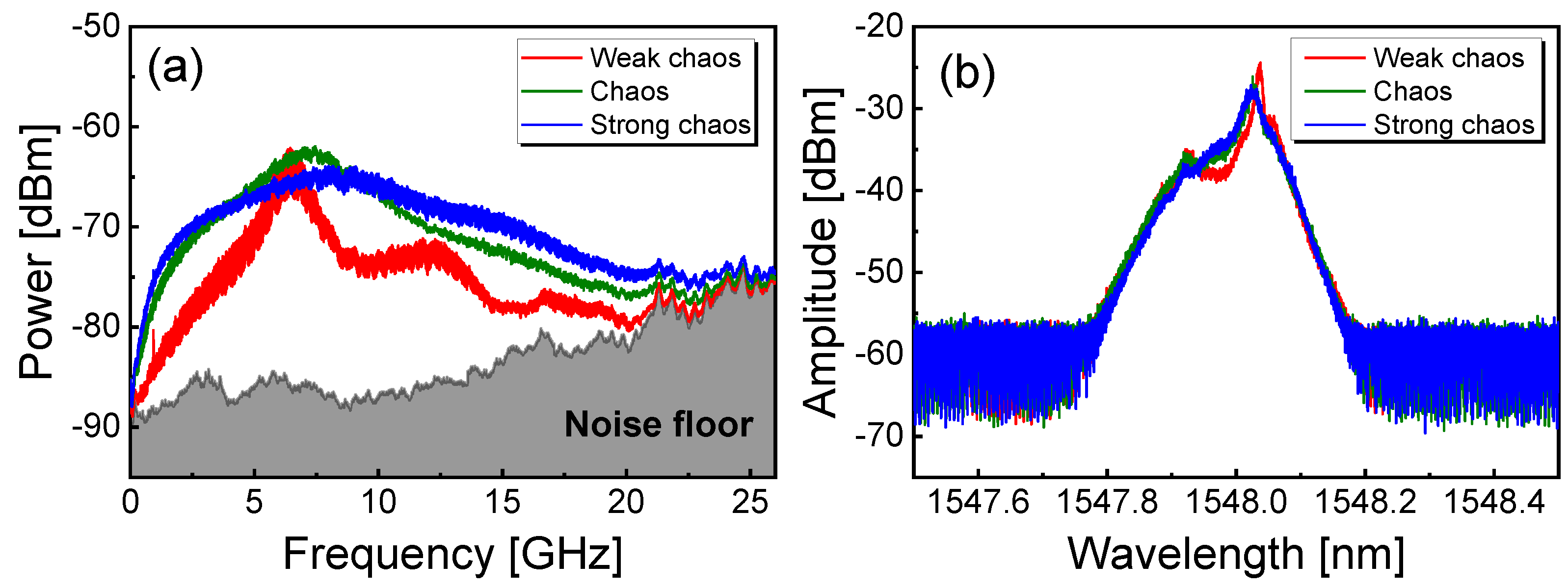
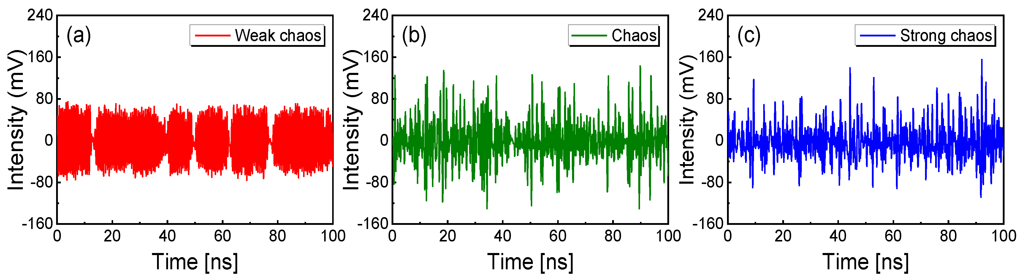
4. Experimental Results

The chaotic laser was firstly attenuated by a variable attenuator and then passed through the HBT setup. In the photon detection system, an internal clock triggered two channel gates simultaneously. When a photon was detected on one channel, the arriving time was recorded. During the same clock period, a subsequent photon was received from another channel and then the time interval was measured. The desired distribution was obtained with many records, and if the detection quantum efficiency was higher, the better the photon pair distribution was close to the real light source distribution. Otherwise, the single photon detector would mistake dark noise for photon signals. Moreover, as the incident photon number increased, the noise level would be higher due to the after pulsing effect. In that case, the time interval distribution of photon pairs was also affected by noise. When the coherence time of light source was short, high resolution time was required in the detection. Besides, the unbalance of the two light intensities after the BS had an adverse effect on the acquired distribution. It was difficult to obtain an accurate time interval distribution of photon pairs with a very low quantum efficiency. In our experiment, the detection quantum efficiency was 25%. We investigated how different average photon intensity and coherence time affected the accuracy of different order corrections. We used the relative error to compare different high order corrections with the ideal second order photon correlation. According to Equation (2), we calculated P₉(τ) with high order terms and omitted the terms higher than ninth order. Likewise, we took the photon pair time interval distribution D₁(τ) and then convolved D₁(τ) to D₉(τ). The terms higher than ninth order were also omitted. Using Equation (17) we obtained a different high order correction of g⁽²⁾(τ) with experimental data. The influences of different average photon intensity and the coherence time were investigated theoretically.

At 1.5 times the threshold current (J = 1.5J_th) and 25 °C temperature (T = 25 °C), central wavelength was stabilized near 1548 nm. We adjusted the attenuator VA1 and polarization controller to accurately control the optical feedback strength. The feedback strength η was obtained as the ratio of the feedback power to the output power of the laser. With the increase of the feedback strength, the laser experienced a transition from period-1 and period-2, to the steady chaos oscillation. Among them, we selected three typical states, including period-2 (weak chaos) with the feedback strength η of 2.66%, the intermediate chaotic state (chaos) with η of 8.87%, and steady chaotic oscillation state (strong chaos) with η of 30.31%. Figure 2a shows the three typical frequency spectrums of the chaotic laser. To quantify the bandwidth of the chaotic laser, we used the definition that is expounded as the frequency spectrum region the DC and the frequency where 80% of the energy is contained within [46]. According to the 80% bandwidth definition, the bandwidth of the chaotic laser was 4.98 GHz, 9.84 GHz, and 11.71GHz, respectively. Figure 2b is the optical spectrum of the chaotic laser. Environmental changes slightly influenced the optical feedback strength and the coherence length [47]. Based on the repeated measurements we obtained the range of coherent time variation. Figure 3 is the three corresponding time series of the chaotic laser.

The bandwidth of the chaotic laser was in the order of GHz and we obtained the coherence time of chaotic laser through 3dB linewidth spectrum. Considering that the ninth order correction of the second order photon correlation g⁽²⁾(τ) was close enough to the theoretical limit, we experimentally took the ninth order correction within 10 ns and theoretically employed the same order fitting. The experimental photon correlations g⁽²⁾(τ) were fitted by ideal expressions, as shown in Figure 4. For photon-bunching chaotic light, the g⁽²⁾(τ) can be written as g⁽²⁾(τ) = 1 + bexp(−2τ/τ_c) (b: bunching amplitude, τ_c: coherence time) [23]. Figure 4 shows the experimental and theoretical fitting results for weak chaos (b = 0.479, τ_c = 0.768 ns), chaos (b = 0.524, τ_c = 0.651 ns), and strong chaos (b = 0.626, τ_c = 0.535 ns).

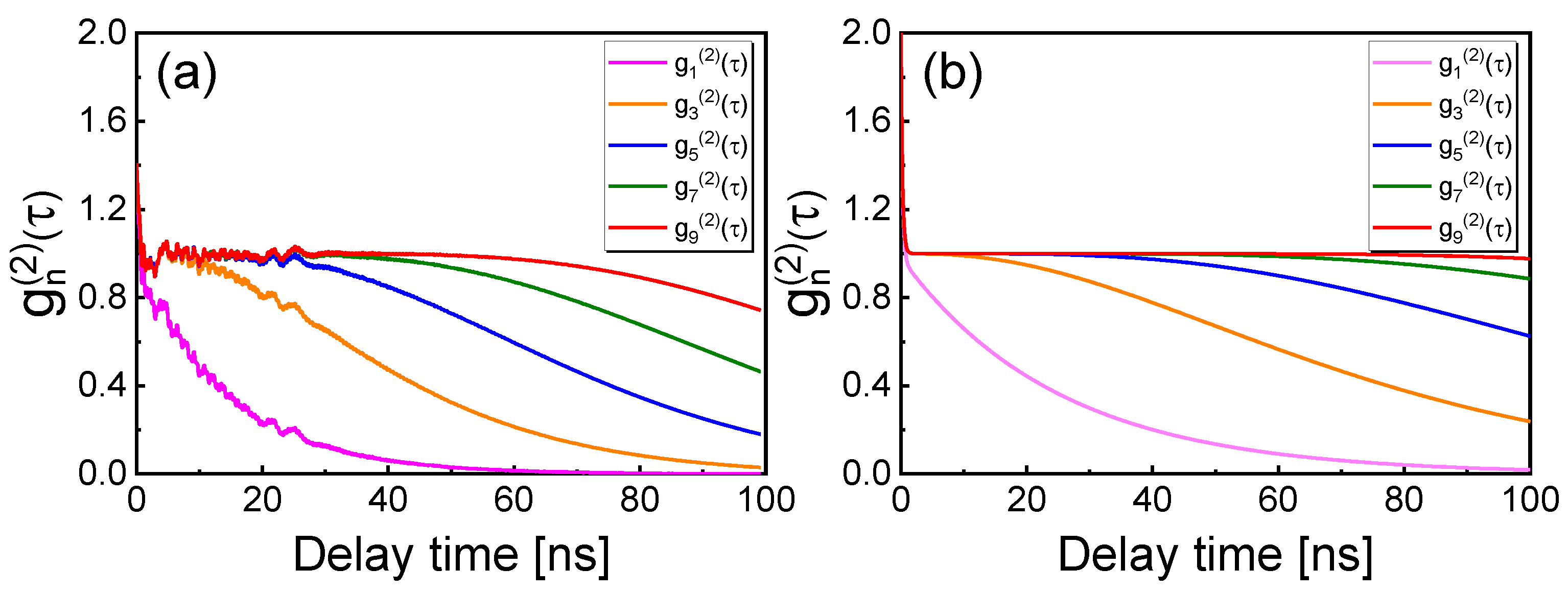
5. Influences of Detector Time Resolution and High Order Omitted Terms

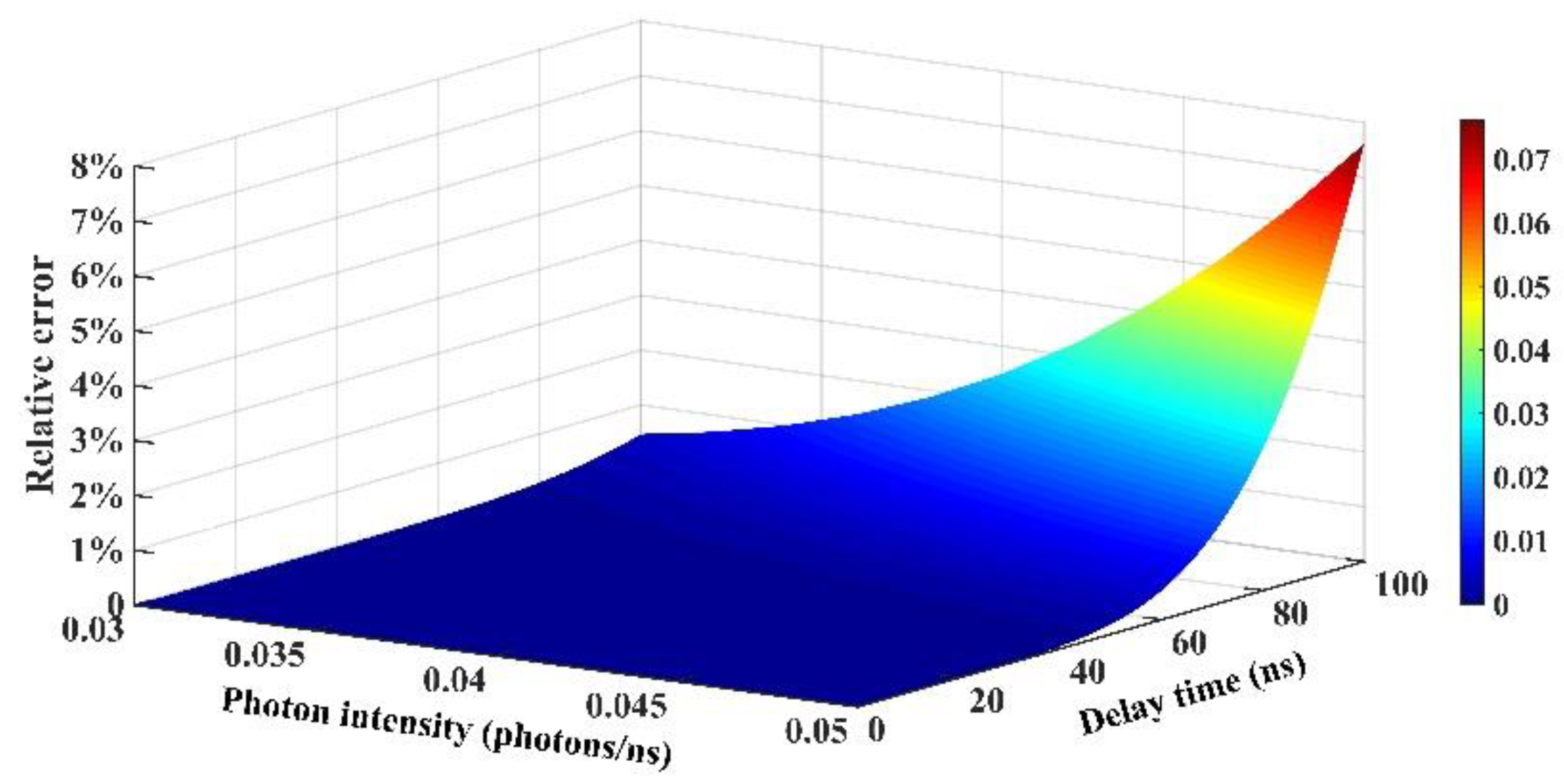
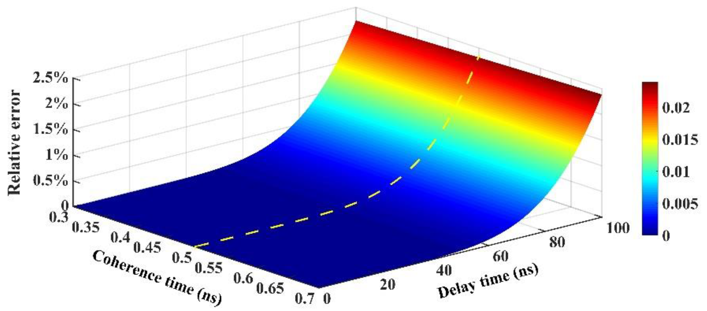
In our experiment, the resolution time of the detection (65 ps) was not significantly small compared to the coherence time (~0.5 ns) of the chaotic laser, resulting in a little fluctuation of measured g⁽²⁾(τ). In Figure 5a, the experimental results of $g_n^{\left(2\right)}$(τ) within 100 ns delay time is shown and the magenta curve represents the original photon pair time interval distribution. The original experimental data is the same as those used in Figure 4b. The bottom-up colored curves indicate the increasing order corrections of second order photon correlation. The orange curve is the third order correction of g⁽²⁾(τ), and the others are fifth, seventh, and ninth order corrections of g⁽²⁾(τ). For an accurate measurement of photon correlation, a very low photon flux rate $\overline{I}$ was required to ensure $\overline{I}{\tau }_c$ < 1 [39]. The counting rate of the SPD was controlled below 0.3 Mcounts/s by using the VA2 and the overall detection efficiency was 25%. In Figure 5a, the counting rate was 270 kcounts/s and the dead time of the SPD was 4 μs. Within 100 ns sampling time (i.e., τ = 100 ns), the incident light intensity was estimated to be about 4 × 10⁷ photons/s. Figure 5b shows the theoretical results when τ_c was 0.5 ns and the incident light intensity was 4 × 10⁷ photons/s. The experimental results are in good agreement with the theory.

6. Relative Error of ${\mathit{g}}_{\mathit{n}}^{\mathbf{\left(}\mathbf{2}\mathbf{\right)}}$(τ) With Mean Photon Intensity and Coherence Time of the Chaotic Laser

The coherence time of our experiment was below 1 ns and we can set the maximum coherence time in the theoretical analysis. Following this, g⁽²⁾(τ) was obtained by using Equation (6), which is independent on the mean photon intensity. Furthermore, according to Equation (18), it is found that the mean photon intensity and coherence time have effects on the relative error. The maximum photon intensity in our experiment did not exceed 0.05 photons/ns. Given this finding, we changed the mean photon intensity from 0.03 photons/ns to 0.05 photons/ns. For the low order correction of g⁽²⁾(τ), it cannot provide sufficient information and accuracy according to Equation (2). For the ninth order correction, there was almost no difference between $g_9^{\left(2\right)}$(τ) and g⁽²⁾(τ) and the loss information can be ignored. Figure 6 shows the relative error of $g_9^{\left(2\right)}$(τ) for photon intensity changes from 0.03 photons/ns to 0.05 photons/ns and different delay times with the ninth order correction. The relative error varied with the photon intensity and delay time. When the delay time is shorter than 40 ns the relative error can be ignored, while the relative error is increased when the delay time is close to 100 ns. It should be noted that higher order correction can reduce the relative error for longer delay time. In Figure 6, it is also indicated that larger photon intensity brings bigger error. But when the photon intensity is too low, the photon pair time interval distribution contains a lot of dark noise that deteriorates the detection performance.

Following this, we theoretically analyzed the coherence time from 0.3 ns to 0.7 ns under the condition that the photon intensity was near 4 × 10⁷ photons/s. Figure 7 shows the relative error as functions of the coherence time τ_c and the delay time τ. The coherence time τ_c varied from 0.3 ns to 0.7 ns and the delay time τ was within 100 ns. In this case, corresponding to our experimental condition, the relative error did not exceed 5‰ within 50 ns delay time. It is worth noting that a long τ_c leads to big relative error, but the change of relative error was subtle. The relative error caused by the coherence time was smaller than that of the photon intensity.

We compared the relative error caused by the above two factors (photon intensity and coherence time). The yellow dashed line in Figure 7 indicates the case that the coherence time was 0.5 ns, which corresponds to the experiment condition. For the same delay time, the relative error caused by coherence time was lower than that caused by photon intensity. Thus, high accuracy g⁽²⁾(τ) requires well controlling the photon intensity [24].

From the above discussion, the high order correction of second order photon correlation was affected by the variations of the mean photon intensity and coherence time of the laser, and we analyzed the relative error caused by the two factors respectively. The relative error from incident photon intensity was larger than that from coherence time. In Figure 7, the dashed line on the error surface was under the condition that the intensity was 0.04 photons/ns and τ_c was 0.5 ns, which corresponds to the experimental condition. In our experiment, the maximum relative error in ninth order correction of g⁽²⁾(τ) did not exceed 5‰ within 50 ns delay time. The relative errors caused by the photon intensity and coherence time retained the uncertainty ±0.01 photon/ns and ±0.2 ns respectively, and the overall error within 50 ns delay time did not exceed 1% in our condition.

7. Conclusions

In conclusion, we precisely measured the second order photon correlation g⁽²⁾(τ) of a chaotic semiconductor laser using self-convolution HBT interferometer. Based on the theoretical analysis, the ninth order self-convolution correction was sufficient to obtain experimentally the accurate g⁽²⁾(τ) from the photon pair time interval distribution. The experimental results were in good agreement with the theory. The relative error caused by coherence time and mean photon intensity was analyzed, which was no more than 5‰ within 50 ns delay time. As the order of convolution increased, the accuracy improved within a long delay time. In comparison with the traditional HBT measurement, this technique, which does not require high intensity and long optical or electric delay, is more useful for a weak light source, such as atomic fluorescence and single photon emission, whose quantum correlation is difficult to be detected. It is demonstrated that this technique provides a new way to measure high order quantum coherence precisely and will bridge the gap between nonlinear optics of chaotic lasers and quantum physics.

References

1. Soriano, M.C.; García-Ojalvo, J.; Mirasso, C.R.; Fischer, I. Complex photonics: Dynamics and applications of delay-coupled semiconductors lasers. Rev. Mod. Phys. 2013, 85, 421–470. [Google Scholar] [CrossRef]
2. Sciamanna, M.; Shore, K.A. Physics and applications of laser diode chaos. Nat. Photonics. 2015, 9, 151–162. [Google Scholar] [CrossRef]
3. VanWiggeren, G.D.; Roy, R. Communication with chaotic lasers. Science 1998, 279, 1198–1200. [Google Scholar] [CrossRef] [PubMed]
4. Argyris, A.; Syvridis, D.; Larger, L.; Annovazzi-Lodi, V.; Colet, P.; Fischer, I.; García-Ojalvo, J.; Mirasso, C.R.; Pesquera, L.; Shore, K.A. Chaos-based communications at high bit rates using commercial fibre-optic links. Nature 2005, 438, 343–346. [Google Scholar] [CrossRef] [PubMed]
5. Hong, Y.; Lee, M.W.; Paul, J.; Spencer, P.S.; Shore, K.A. Enhanced chaos synchronization in unidirectionally coupled vertical-cavity surface-emitting semiconductor lasers with polarization-preserved injection. Opt. Lett. 2008, 33, 587–589. [Google Scholar] [CrossRef] [PubMed]
6. Wu, J.G.; Wu, Z.M.; Xia, G.Q.; Deng, T.; Lin, X.D.; Tang, X.; Feng, G.Y. Isochronous synchronization between chaotic semiconductor lasers over 40-km fiber links. IEEE Photon. Technol. Lett. 2011, 23, 1854–1856. [Google Scholar] [CrossRef]
7. Lavrov, R.; Jacquot, M.; Larger, L. Nonlocal nonlinear electro-optic phase dynamics demonstrating 10 Gb/s chaos communications. IEEE J. Quantum Electron. 2010, 46, 1430–1435. [Google Scholar] [CrossRef]
8. Yoshimura, K.; Davis, J.P.; Harayama, T.; Okumura, H.; Morikatsu, S.; Aida, H.; Uchida, A. Secure key distribution using correlated randomness in lasers driven by common random light. Phys. Rev. Lett. 2012, 108, 070602. [Google Scholar] [CrossRef]
9. Uchida, A.; Amano, K.; Inoue, M.; Hirano, K.; Naito, S.; Someya, H.; Oowada, I.; Kurashige, T.; Shiki, M.; Yoshimori, S.; et al. Fast physical random bit generation with chaotic semiconductor lasers. Nat. Photonics 2008, 2, 728–732. [Google Scholar] [CrossRef]
10. Reidler, I.; Aviad, Y.; Rosenbluh, M.; Kanter, I. Ultrahigh-speed random number generation based on a chaotic semiconductor laser. Phys. Rev. Lett. 2009, 103, 024102. [Google Scholar] [CrossRef]
11. Kanter, I.; Aviad, Y.; Reidler, I.; Cohen, E.; Rosenbluh, M. An optical ultrafast random bit generator. Nat. Photonics 2010, 4, 58–61. [Google Scholar] [CrossRef]
12. Wang, A.B.; Li, P.; Zhang, J.G.; Zhang, J.Z.; Li, L.; Wang, Y.C. 4.5 Gbps high-speed real-time physical random bit generator. Opt. Express 2013, 21, 20452–20462. [Google Scholar] [CrossRef] [PubMed]
13. Brunner, D.; Soriano, M.C.; Mirasso, C.R.; Fischer, I. Parallel photonic information processing at gigabyte per second data rates using transient states. Nat. Commun. 2013, 4, 1364. [Google Scholar] [CrossRef] [PubMed]
14. Lin, F.Y.; Liu, J.M. Chaotic radar using nonlinear laser dynamics. IEEE J. Quantum Electron. 2004, 40, 815–820. [Google Scholar] [CrossRef]
15. Wang, Y.C.; Wang, B.J.; Wang, A.B. Chaotic correlation optical time domain reflectometer utilizing laser diode. IEEE Photon. Technol. Lett. 2008, 20, 1636–1638. [Google Scholar] [CrossRef]
16. Xia, L.; Huang, D.; Xu, J.; Liu, D. Simultaneous and precise fault locating in WDM-PON by the generation of optical wideband chaos. Opt. Lett. 2013, 38, 3762–3764. [Google Scholar] [CrossRef]
17. Heil, T.; Fischer, I.; Elsässer, W.; Mulet, J.; Mirasso, C.R. Statistical properties of low-frequency fluctuations during single-mode operation in distributed-feedback lasers: experiments and modeling. Opt. Lett. 1999, 24, 1275–1277. [Google Scholar] [CrossRef]
18. Sukow, D.W.; Heil, T.; Fischer, I.; Gavrielides, A.; Hohl-AbiChedia, A.; Elsässer, W. Picosecond intensity statistics of semiconductor lasers operating in the low-frequency fluctuation regime. Phys. Rev. A. 1999, 60, 667–673. [Google Scholar] [CrossRef]
19. Li, N.; Kim, B.; Locquet, A.; Choi, D.; Pan, W.; Citrin, D.S. Statistics of the optical intensity of a chaotic external-cavity DFB laser. Opt. Lett. 2014, 39, 5949–5952. [Google Scholar] [CrossRef]
20. Heiligenthal, S.; Dahms, T.; Yanchuk, S.; Jüngling, T.; Flunkert, V.; Kanter, I.; Schöll, E.; Kinzel, W. Strong and Weak Chaos in Nonlinear Networks with Time-Delayed Couplings. Phys. Rev. Lett. 2011, 107, 234102. [Google Scholar] [CrossRef]
21. Porte, X.; Soriano, M.C.; Fischer, I. Similarity properties in the dynamics of delayed-feedback semiconductor lasers. Phys. Rev. A. 2014, 89, 023822. [Google Scholar] [CrossRef]
22. Oliver, N.; Soriano, M.C.; Sukow, D.W.; Fischer, I. Dynamics of a semiconductor laser with polarization-rotated feedback and its utilization for random bit generation. Opt. Lett. 2011, 36, 4632–4634. [Google Scholar] [CrossRef] [PubMed]
23. Albert, F.; Hopfmann, C.; Reitzenstein, S.; Schneider, C.; Höfling, S.; Worschech, L.; Kamp, M.; Kinzel, W.; Forchel, A.; Kanter, I. Observing chaos for quantum-dot microlasers with external feedback. Nat. Commun. 2011, 2, 366. [Google Scholar] [CrossRef] [PubMed]
24. Guo, Y.Q.; Peng, C.S.; Ji, Y.L.; Li, P.; Guo, Y.Y; Guo, X.M. Photon statistics and bunching of a chaotic semiconductor laser. Opt. Express 2018, 26, 5991–6000. [Google Scholar] [CrossRef]
25. Hanbury Brown, R.; Twiss, R.Q. Correlation between photons in two coherent beams of light. Nature 1956, 177, 27–29. [Google Scholar] [CrossRef]
26. Glauber, R.J. Photon Correlations. Phys. Rev. Lett. 1963, 10, 84–86. [Google Scholar] [CrossRef]
27. Glauber, R.J. The Quantum Theory of Optical Coherence. Phys. Rev. 1963, 130, 2529–2539. [Google Scholar] [CrossRef]
28. Glauber, R.J. Coherent and Incoherent States of the Radiation Field. Phys. Rev. 1963, 131, 2766–2788. [Google Scholar] [CrossRef]
29. Arecchi, F.T. Measurement of the statistical distribution of Gaussian and laser sources. Phys. Rev. Lett. 1965, 15, 912–916. [Google Scholar] [CrossRef]
30. Kimble, H.; Dagenais, J.M.; Mandel, L. Photon antibunching in resonance fluorescence. Phys. Rev. Lett. 1977, 39, 691–695. [Google Scholar] [CrossRef]
31. Oberreiter, L.; Gerhardt, I. Light on a beam splitter: More randomness with single photons. Laser Photonics Rev. 2016, 10, 108–115. [Google Scholar] [CrossRef] [Green Version]
32. Sun, F.-W.; Shen, A.; Dong, Y.; Chen, X.D.; Guo, G.C. Bunching effect and quantum statistics of partially indistinguishable photons. Phys. Rev. A. 2017, 96, 023823. [Google Scholar] [CrossRef] [Green Version]
33. Schultheiss, V.H.; Batz, S.; Peschel, U. Hanbury Brown and Twiss measurements in curved space. Nat. Photonics 2016, 10, 106–110. [Google Scholar] [CrossRef]
34. Smith, T.A.; Shih, Y. Turbulence-Free Double-slit Interferometer. Phys. Rev. Lett. 2018, 120, 063606. [Google Scholar] [CrossRef]
35. Chen, X.H.; Agafonov, I.N.; Luo, K.H.; Liu, Q.; Xian, R.; Chekhova, M.V.; Wu, L.A. High-visibility, high-order lensless ghost imaging with thermal light. Opt. Lett. 2010, 35, 1166–1168. [Google Scholar] [CrossRef] [Green Version]
36. Zhou, Y.; Simon, J.; Liu, J.; Shih, Y. Third-order correlation function and ghost imaging of chaotic thermal light in the photon counting regime. Phys. Rev. A. 2010, 81, 043831. [Google Scholar] [CrossRef]
37. Ryczkowski, P.; Barbier, M.; Friberg, A.T.; Dudley, J.M.; Genty, G. Ghost imaging in the time domain. Nat. Photonics 2016, 10, 167–170. [Google Scholar] [CrossRef]
38. Magaña-Loaiza, O.S.; Mirhosseini, M.; Cross, R.M.; Hashemi Rafsanjani, S.M.; Boyd, R.W. Hanbury Brown and Twiss interferometry with twisted light. Sci. Adv. 2016, 2, e1501143. [Google Scholar] [CrossRef] [Green Version]
39. Guo, Y.Q.; Li, G.; Zhang, Y.F.; Zhang, P.F.; Wang, J.M.; Zhang, T.C. Efficient fluorescence detection of a single neutral atom with low background in a microscopic optical dipole trap. Sci. China: Phys. Mech. Astron. 2012, 55, 1523–1528. [Google Scholar] [CrossRef]
40. Loudon, R. Quantum degrees of first and second-order coherence. In The Quantum Theory of Light, 3rd ed.; Oxford University Press: New York, NY, USA, 2000; pp. 176–178. [Google Scholar]
41. Boitier, F.; Godard, A.; Rosencher, E.; Fabre, C. Measuring photon bunching at ultrashort timescale by two-photon absorption in semiconductors. Nat. Phys. 2009, 5, 267–270. [Google Scholar] [CrossRef]
42. Nevet, A.; Hayat, A.; Ginzburg, P.; Orenstei, M. Indistinguishable photon pairs from independent true chaotic sources. Phys. Rev. Lett. 2011, 107, 253601. [Google Scholar] [CrossRef] [PubMed]
43. Bai, B.; Liu, J.; Zhou, Y.; Zheng, H.; Chen, H.; Zhang, S.; He, Y.; Li, F.; Xu, Z. Photon superbunching of classical light in the Hanbury Brown–Twiss interferometer. J. Opt. Soc. Am. B 2017, 34, 2081–2088. [Google Scholar] [CrossRef] [Green Version]
44. Huang, C.H.; Wen, Y.H.; Liu, Y.W. Measuring the second order correlation function and the coherence time using random phase modulation. Opt. Express 2016, 24, 4278–4288. [Google Scholar] [CrossRef] [PubMed] [Green Version]
45. Beck, M. Comparing measurements of g(2)(0) performed with different coincidence detection techniques. J. Opt. Soc. Am. B 2007, 24, 2972–2978. [Google Scholar] [CrossRef]
46. Lin, F.Y.; Liu, J.M. Nonlinear dynamical characteristics of an optically injected semiconductor laser subject to optoelectronic feedback. Optics Commun. 2003, 221, 173–180. [Google Scholar] [CrossRef]
47. Wang, Y.; Kong, L.; Wang, A.; Fan, L. Coherence length tunable semiconductor laser with optical feedback. Appl. Optics 2009, 48, 969–973. [Google Scholar] [CrossRef]
Figure 1. Schematic diagram of the experimental setup for measuring photon correlation g(2)(τ) of a chaotic optical-feedback laser. DFB-LD: distributed feedback 1550 nm laser diode; PC: polarization controller; OC: optical circulator; VA1 and VA2: variable optical fiber attenuator; FC1 and FC2: fiber coupler; PD: high-speed photodetector; L1, L2 and L3: aspheric lens collimator; BS: beam splitter; F: optical filter; SPD: single photon detector; TDC: time to digital converter; LC: laptop computer; OSC: oscilloscope; TTC: thermoelectric temperature controller; CSC: current source controller.
Applsci 09 04907 g001
Figure 2. (a) Measured frequency spectrum and (b) optical spectrum of the chaotic laser, when J = 1.5Jth and η = 2.66% (weak chaos), 8.87% (chaos), 30.31% (strong chaos).
Applsci 09 04907 g002
Figure 3. Measured three corresponding time series of the chaotic laser. The bias current J = 1.5Jth and feedback strength (a) η = 2.66%, (b) 8.87%, (c) 30.31% are the same as those used in Figure 2.
Applsci 09 04907 g003
Figure 4. The ninth order correction of second order photon correlation and the theoretical fitting. The bias current J = 1.5Jth and feedback strength (a) η = 2.66%, (b) 8.87%, (c) 30.31% are the same as those used in Figure 2.
Applsci 09 04907 g004
Figure 5. The (a) experimental and (b) theoretical results of g n ( 2 ) ( τ ) within the delay time 100 ns.
Applsci 09 04907 g005
Figure 6. The relative error varying with the photon intensity and delay time. The coherence time is set as one ns.
Applsci 09 04907 g006
Figure 7. Relative error as functions of coherence time and delay time. The photon intensity was 0.04 photons/s and the yellow dashed line corresponds to the experimental condition.
Applsci 09 04907 g007