Enhancing Decision Making through Combined Classification Techniques and Probabilistic Data Analysis for Ubiquitous Healthcare Anomaly Monitoring

Abstract

A multi-agent data-analytics-based approach to ubiquitous healthcare monitoring is presented in this paper. The proposed architecture gathers a patient’s vital data using wireless body area networks, and the transmitted information is separated into binary component parts and divided into related dataset categories using several classification techniques. A probabilistic procedure is then used that applies a normal (Gaussian) distribution to the analysis of new medical entries in order to assess the gravity of the anomalies detected. Finally, a data examination is carried out to gain insight. The results of the model and simulation show that the proposed architecture is highly efficient in applying smart technologies to a healthcare system, as an example of a research direction involving the Internet of Things, and offers a data platform that can be used for both medical decision making and the patient’s wellbeing and satisfaction with their medical treatment.

1. Introduction

Recent innovative works and research progress in the area of integrated circuits, wireless communications and sensors have allowed the creation of smart devices. Many fields now use a number of these devices, for example ubiquitous healthcare systems. The omnipresence of heterogeneous technologies has opened the way for better approaches to solving many current issues related to connected devices, and has highlighted the importance of the Internet of Things. Smart connected sensors are principal components of wireless body area networks (WBANs) and biosensors, and are fast becoming a key aspect of the Internet of Things. A WBAN is an emerging technology consisting of tiny sensors and medical devices placed on the bodies of humans or animals. It connects wirelessly to sense vital signs, and allows the remote, real-time diagnosis of health issues. Technologies used in association with wireless sensor networks and the Internet of Things are closely linked to many fields, such as e-health [1], gaming, sports [2], military [3] and many applications are built in protected agriculture [4]. A recent medical study reports that the average age of the populations of developing countries is increasing [5]. Healthcare organizations are faced with the issue of a significantly larger elderly populace [6,7], which is becoming a major worldwide health problem. Ubiquitous systems offer the possibility of simplifying and easing access to health services [8], especially at the end of intensive care. Through collaboration between these smart systems, WBANs offer a number of medical sensors that are capable of gathering vital physiological information such as blood pressure, heart rate, oxygen saturation, etc. and then transmitting these data wirelessly to be analyzed for a given process and task. In order to ensure the wellbeing of patients with chronic diseases, hospitals, smart homes and medical centers need to be equipped with a wide assortment of e-health solutions and connected medical devices. Hypertension as an example is a frequent health issue that has no evident symptoms; It is therefore important to monitor blood pressure regularly, as the only way to control its changes is to be on medications. The classification of medical abnormalities such as hypertension involves detecting and classifying data samples that present a problem or a danger to a patient’s health. The use of multi-agent systems is a research trend that can help to solve problems that are difficult for a monolithic system to deal with. The aim of our approach is to help medical staff to diagnose health disorders, and to detect or predict anomalies and seizures. The system proposed in this paper uses a specific classification model for each patient, meaning that decision making is specific, and on a case-by-case basis. The Gaussian distribution applied in this work takes into account various detected anomalies in order to analyze them. This facilitates learning of the behavior and habits of a patient while guiding the medical treatments that can alleviate any medical conditions. Statistics is used in many everyday applications, and many machine learning and data mining systems assume that data fed to these models follow a normal (Gaussian) distribution, allowing inferences to be made from a sample to a parent population. To support the results obtained, a comparative study between different classification techniques is illustrated in the results section.

Despite continuous research and improvement efforts from industry, wireless sensor networks face many issues associated with network topologies, energy usage and restricted resources. These sensors are placed in, on or around a patient’s body in order to gather and transmit medical information such as electrocardiograms (ECGs), blood pressure (BP), movement and so on [9]. Figure 1 illustrates a WBAN architecture applied to healthcare detailing different communications types. The applications of WBANs are diverse, and range from e-health and ambient assisted living to mobile health and sports training.

Wireless sensor networks provide a communication framework that enables the sensing, gathering and forwarding of data to a central destination for further data analysis and decision making [10]. One of the main concerns in these networks is to guarantee their energy efficiency for as long as possible. This collection of sensors can be linked with the Internet of Things to provide innovative applications for scientific research purposes. In order to develop our smart system, we combine many fields of computer science such as wireless sensor networks, classification techniques and probabilistic approaches. The proposed architecture consists of a smart connected system for ubiquitous healthcare applications. The aim is to use WBAN devices as a real-time medical data source and to provide an autonomous intelligent system that is capable of monitoring patients in a medical setting.

Table 1. Most used medical sensors and their technical information.

Sensors	Nomenclature	Technical Specificities
ECG	Electrocardiogram	-
EMG	Electromyography	10 Mb/s
EEG	Electroencephalography	5–10 m
B.P	Blood Pressure	~50 mW

summarizes the nomenclature and the technical specificities of the main used sensors in a single or multiple-WBAN environment. It is important to note that this research work focuses on the BP-related sensor. The other sensors such as ECG, EMG and EEG are shown for information purposes only. In this paper, we examine only on-body area networks; blood pressure sensors belong to this group, since these devices are attached to a patient.

Currently, one of the top challenges that every country is facing is healthcare [11]. Numerous ubiquitous healthcare structures are outlined here and various different perspectives are taken into consideration, such as the reliability of the vital patient information to be transmitted, and the lifetime and monitoring of battery utilization based on optimized routing protocols [12]. There is a rapidly growing body of literature on ubiquitous healthcare systems, which highlights its value and contains many examples of research in this field. The objective is to propose a healthcare solution that is capable of monitoring a patient’s vital signs and notifying physicians and/or technicians wirelessly when these metrics exceed certain limits. In this section, we give a brief overview of the state-of-the-art of ubiquitous systems and several examples that are related to our work. In [13,14,15], a ubiquitous healthcare system consisting of physiological data-gathering devices using medical sensors offers monitoring and managing solutions for a patient’s health condition. Several works propose interesting solutions applied to e-health and ubiquitous systems; for example, Kang et al. [16] used EEG sensors in order to classify stress status based on brain signals, while Kim et al. [17] designed a mobile healthcare application based on an image representation of the tongue, a vital muscular organ. A summary of the energy requirements of a WBAN-based real-time healthcare monitoring architecture can be found in Kumar et al. [18]. Hanen et al. [19] implemented a multi-agent system based mobile medical service using the framework for modeling and simulation of cloud computing infrastructures and services (CloudSim). Hamdi et al. [20] created a software system that improved the maintenance management of medical technology by sorting medical maintenance requests. O’Donoghue and Herbert [21] presented a data management system (DMS) architecture, an agent-based middleware that utilizes both hardware/software resources within a pervasive environment and provides data quality management. Lee et al. [22] proposed a management system for diabetes patients based on generated rules and a K-nearest neighbors (KNN) classification technique. Ketan et al. [23] developed a healthcare system for diabetes patients that makes it easier to obtain a rapid diagnosis.

A ubiquitous healthcare system generally comprises of three components:

• A portable bio-signal data-gathering device, represented by wired/wireless connected sensors;
• A device for transmitting previously collected data by communicating with a remote server;
• A server used to investigate the patient’s medical information.

Despite several contributions to significant advances in the world of ubiquitous services, these studies did not provide a data analysis support that can help medical staff to interpret correctly the various changes in a patient’s medical metrics. In addition to medical data classification, our approach fills this need by offering anomaly detection based on the learning model, as well as a probabilistic study that can illustrate in depth the physiological behavior of the patient by comparing the distributions at different critical points throughout the data-recording period.

Our approach therefore meets two key needs:

• Provide a solution adapted to each patient on a case-by-case basis. This therefore implies a single-use learning model for any subject in this analysis and responds to the challenge of generalizing the interpretation of the various medical data in order to provide as accurate a diagnosis as possible (age, environment, habits, etc.)
• Once an anomaly is detected, another classification method has been introduced to assess the severity of the situation. This perfectly meets an immediate need that can regularize medical intervention in the event of a patient’s critical situation.

The remainder of this paper is organized as follows: following this introduction, Section 2 moves on to discuss the methodologies used to implement the proposed architecture. Section 3 carries out an analysis in which the results are interpreted and explained. Section 4 describes the significance of the findings based on the achieved results. Finally, Section 5 presents the conclusion and open areas for research, and proposes potential solutions to issues that are currently faced in this study.

2. Materials and Methods

2.1. System Modeling Process

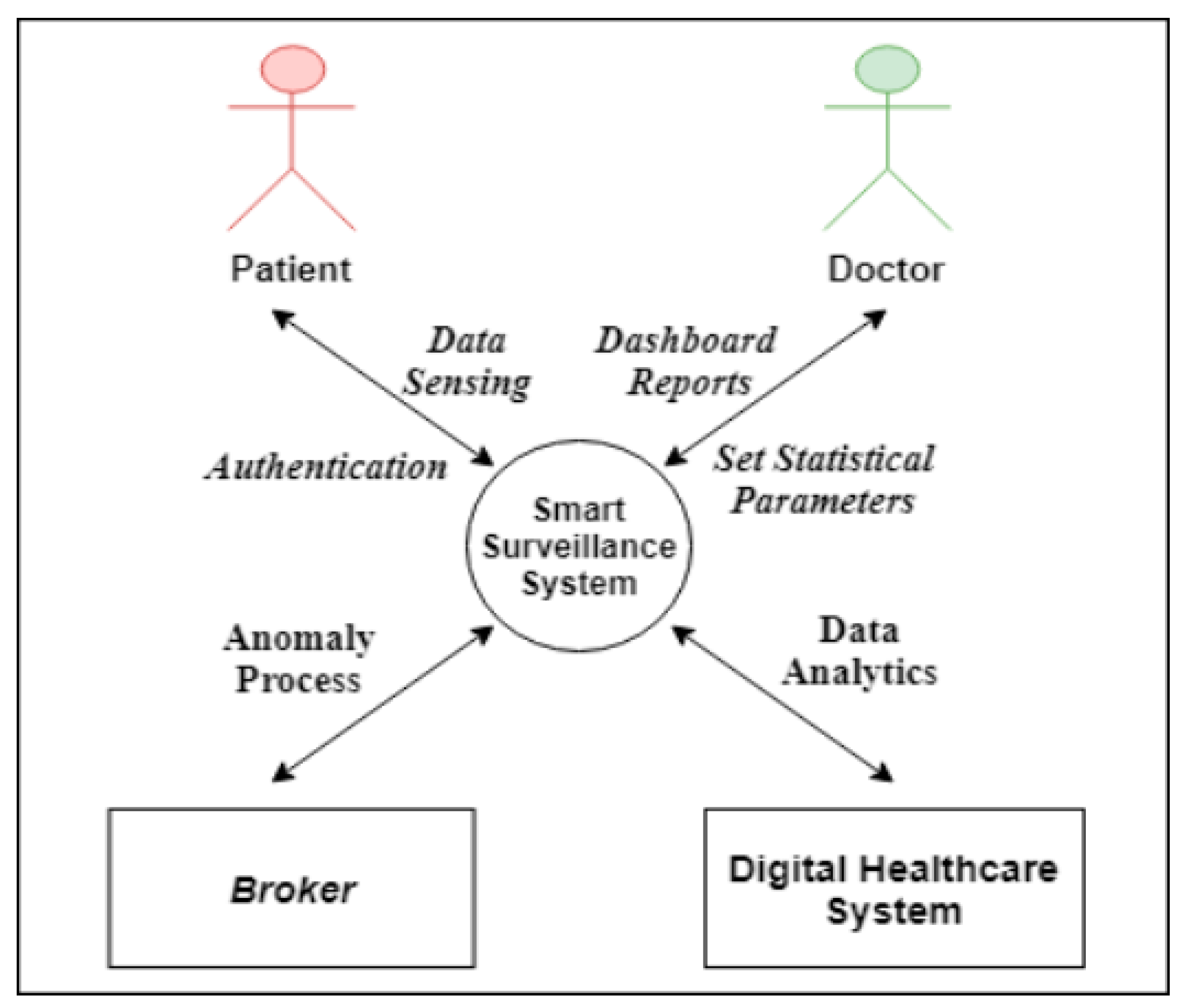
This step consisted of modeling the system using unified modeling language (UML). This helped in an understanding of the static structure and dynamic behavior of our architecture, and allowed us to embed its description techniques into the system model. It conceptualizes the software requirements using a collection of diagrams, and its capability is demonstrated by its easily convertible modeling base, which is applied in many scientific areas such as in describing brain-computer interface (BCI) systems [24] or providing logistic services to ensure smooth and secure transportation [25]. We divided the principal system into two fully connected subsystems, and defined several agents that collaborate to achieve various tasks. The different types of actors in our system included the doctor, the patient and the calculation resources. In this section, the methodology behind this architecture was described using diagrams, and we defined the actors that interacted within our system. Six independent agents worked together to carry out the most critical tasks. This paper highlighted the two major aspects of our system modeling process (SMP): the classification and analytical processes.

• Patient (actor agent);
• Doctor (actor agent);
• Digital health system (DHS; sub-system and system agent);
• Broker (system agent);
• Patient data store (PDS; system agent);
• Data analytics (DA; system agent).

2.1.1. Smart Surveillance System

The principal roles of a smart surveillance system (SSS) are as follows:

• Requesting analytical operations;
• Gathering real-time sensed data;
• Providing dashboard reports for the doctor;

Issuing alerts.

Figure 2 shows a context diagram for the relationship between the system and the other external entities (systems, agents, data stores, etc.).

2.1.2. Digital Health System

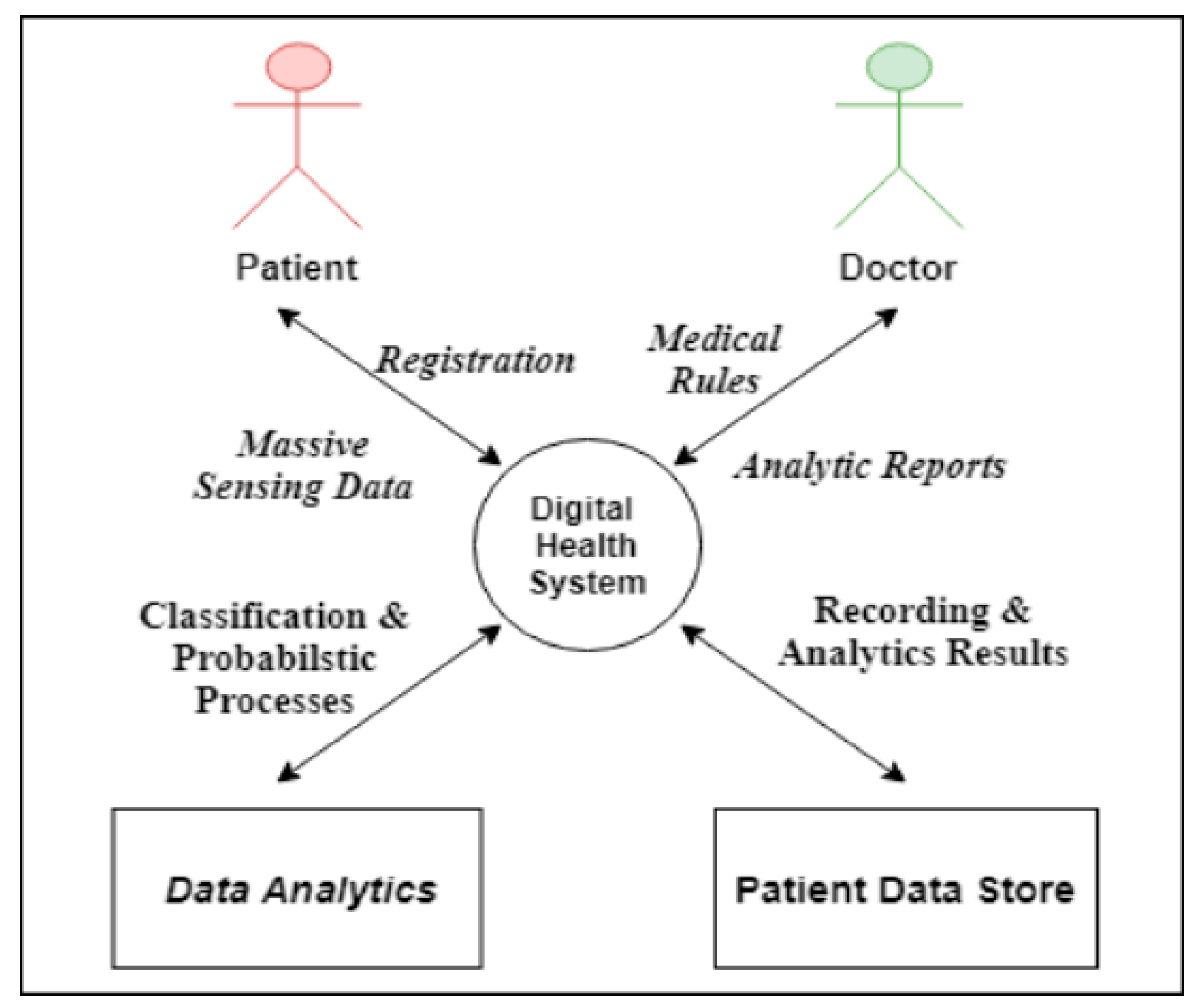
Figure 3 presents a context diagram for the DHS sub-system. Its main functions are as follows:

• Patient authentication;
• Reporting/updating data;
• Classifying vital signs;
• Providing statistical information.

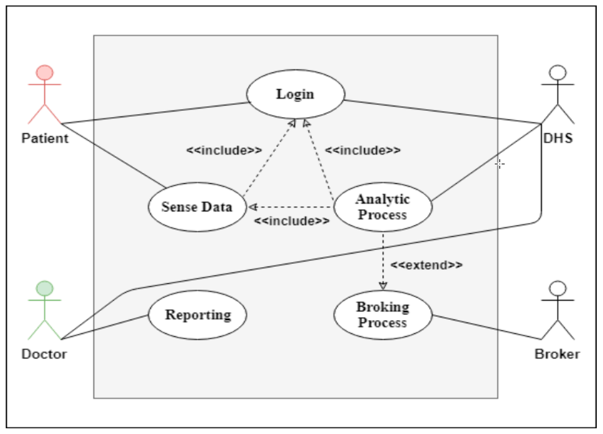
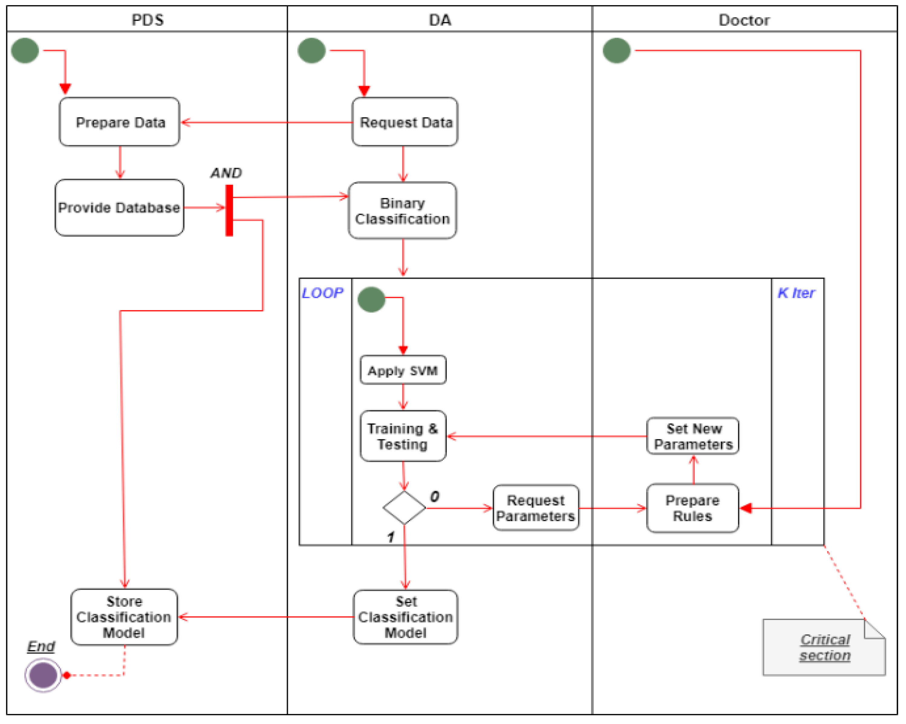
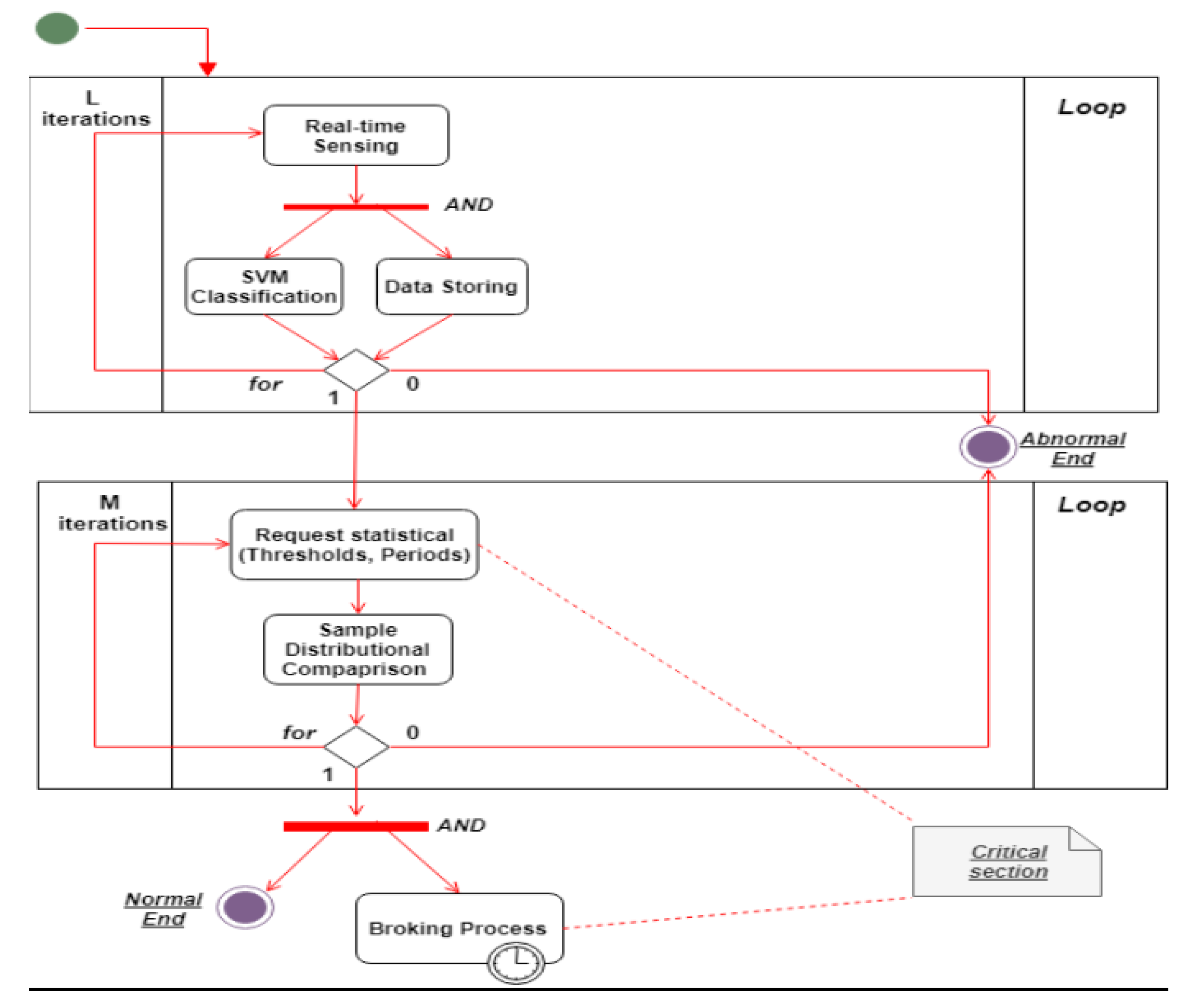
The SSS is illustrated in detail in Figure 2, Figure 4, Figure 5. Figure 4 shows a use case diagram for the SSS that summarizes the goals and the scope of each actor/agent in the system and their interactions via explicit scenarios, while Figure 5 shows the activity diagram for the analytical process use case in the SSS. Its aim was to shape the functional aspect of the system by illustrating the flow from one activity to another. A functional view is presented in this diagram to explain the behavior of each actor throughout the process. The goal was therefore to model the flow of control and data flows. It graphically represents the behavior of the DHS use case. The communication between the patient, PDS, DA and doctor allowed both to process data and save it in the classification model. Between the two processes we applied support vector machine (SVM) to be able to prepare our learning model. Then came the validation phase of the obtained model. This process is therefore vital to the development of a reliable medical model that can be used later when an anomaly is detected.

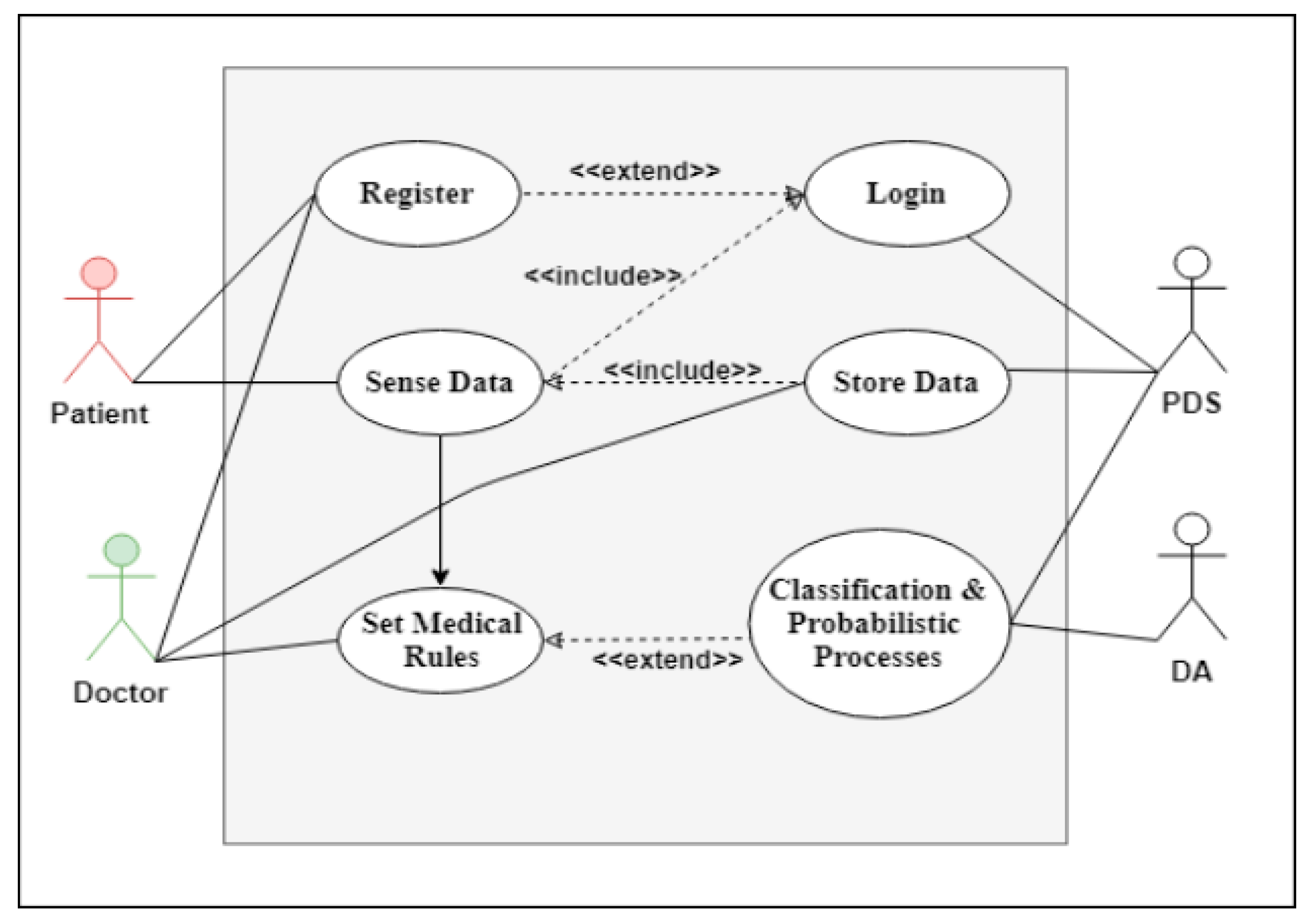
Taken together, these two sub-systems can collaborate to provide a solid platform where data examination is fluid. Four external agents collaborate in the use case diagram shown in Figure 6 and its analogous restricted activity diagram for the classification process in Figure 7. This figure illustrates the relationship between PDS and DA. Since the learning model was ready, it would be used for real-time data classification. If an anomaly was detected, it would be analyzed using the normal distribution. If our model considered the anomaly to be dangerous, then a broking process would be triggered to disseminate the patient’s information and health status.

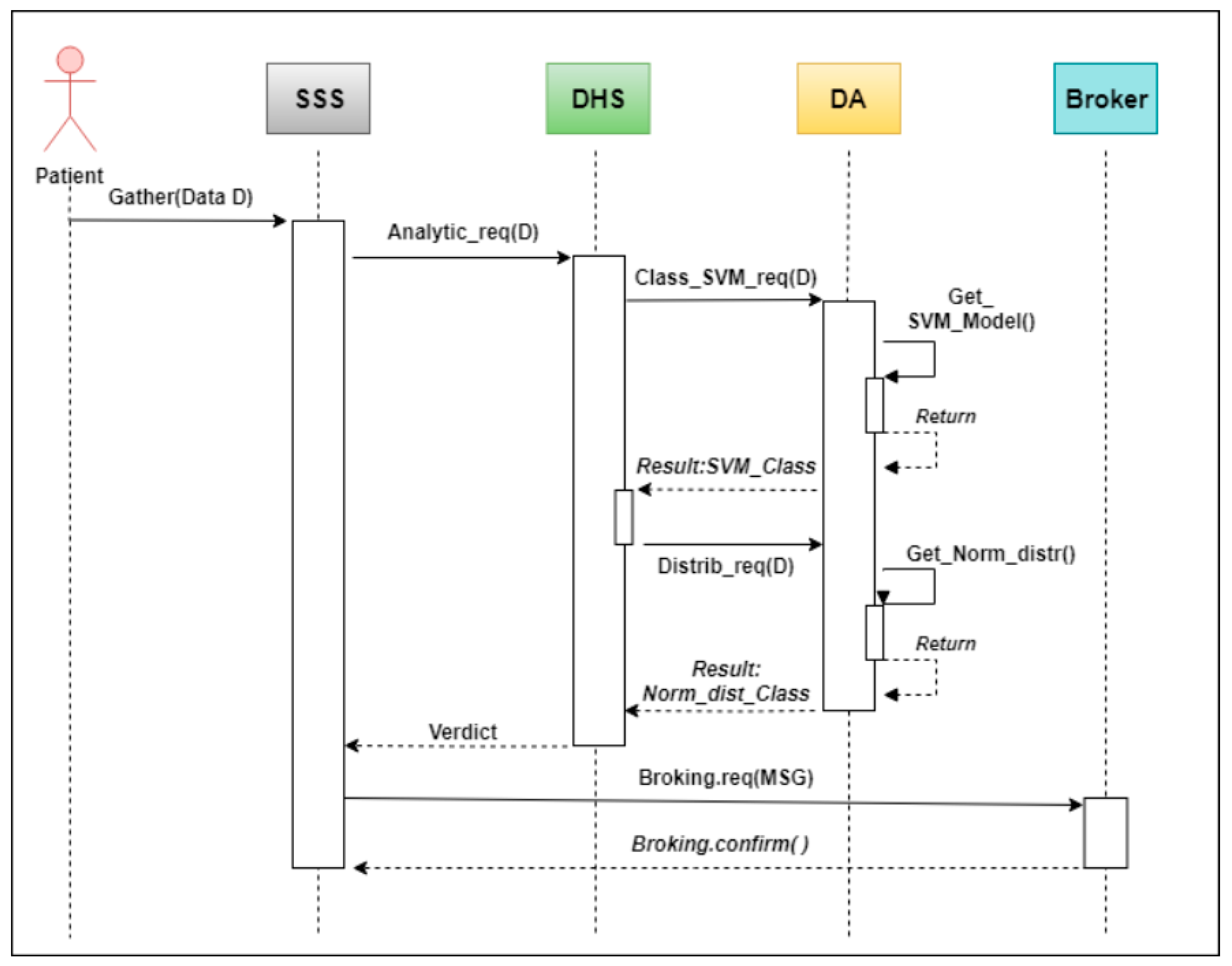
Figure 8 summarizes how medical data are transferred from the patient after being sensed using a WBAN device, through the double classification process mentioned in the next section, and finally to an agent broker, which is responsible for generating an alert of a given severity. An interaction diagram was used for this purpose.

2.1.3. Classification Techniques

As the patient’s sensed vital information was gathered (on a large scale) using WBAN sensors, the DHS periodically stored these data in a transactional database (the PDS) for analysis. The massive scale of data involved made it possible to increase the efficiency of the classification techniques during this process. When a large amount of data is collected, a classification process can be used based on the SVM classifier, which is one of the most widely used algorithms in the medical sciences regarding its satisfactory results in terms of accuracy, precision and recall. The SVM was therefore used to classify blood pressure values as safe (normal) and risky (abnormal). This process requires the application of medical rules that are predefined by the medical staff and/or a binary-based classification that can detect and report the presence of potential anomalies. Our learning model was based during the training process on the following blood pressure references: ideal blood pressure, which is considered as safe and pre-high blood pressure, high blood pressure and low blood pressure that are risky. Once our model was well trained, it would be able to classify any BP value based on the learned knowledge. The generated model could therefore be applied at the SSS level, which uses two different classification techniques in order to assess the degree of danger of the anomalies previously detected. The work in this paper made it possible to initially classify the medical information of a patient in binary mode based on relational criteria. Following this, a second classifier based on a probabilistic approach was used to notify the broker agent. The aim of this was to reconsider the problem in order to quantify it to extract the maximum amount of useful knowledge. This involved switching from a binary mode (safe (0)/risky (1)) to a probabilistic based model. For example, if a B.P reading represents a high value of a blood pressure, which is classified as risky, the probability of its impact relative to a reference value (mean and standard deviation of the same sample) can quantify this anomaly compared to the remaining medical information in order to assess its risk to the patient’s health. This was fully explained in the section entitled “Probabilistic Approach”.

(a)  Data classification using support vector machines:

SVMs are a set of supervised learning techniques that are used for classification, regression and outlier detection [26]. Unlike other classifiers, a SVM finds the optimum line separating the closest points of different classes, called support vectors, and draws this by carrying out vector subtraction.

Table A1. Variables used in the SVM classification process.

Symbol	Variable	Definition Domain
$w$	Weight (unit) vector	-
$\parallel w\parallel$	Norm of $w$	-
x	Feature vector	$\mathrm{x}\in {ℝ}^n$
n	Dimension of x	n ≥ 1
$y_i$	Class of sample	$y_i\in \left\{-1,1\right\}$
$x_i,y_i$	Dataset sample	1≥ i ≥ N
N	Training set	-
K	Kernel function	-
α	Lagrange multiplier	-
b	Scalar value	-
${\mathsf{\epsilon }}_i$	Slack variables	${\mathsf{\epsilon }}_i$≥ 0; i= {1,…..,L}
C	Penalty factor	0 ≥ α ≥ C
$\mathsf{\phi }$	Mapping function	-
$N_{sv}$	Number of support vectors	-

in Appendix A contains a table that defines the variables used during the classification procedure. We obtained the hyper plane separation equation using the following formulae:

$$\mathrm{w}.{\mathrm{x}}_{\mathrm{i}}+\mathrm{b}=0.$$

(1)

Once the linear separation and support vector were obtained, this equation changed to:

$$\mathrm{w}.{\mathrm{x}}_{\mathrm{i}}+\mathrm{b}=\pm 1.$$

(2)

For nonlinear problems, finding the optimal hyper plane depends on solving this minimization problem by introducing penalty parameter and slack variables an introducing the scoring function formula:

$$\mathrm{Min}\frac{1}{2}\parallel \mathrm{w}{\parallel }^2+\mathrm{C}.{{\displaystyle \sum }}_{\mathrm{i}=1}^{\mathrm{n}}{\mathsf{\epsilon }}_{\mathrm{i}};{{\displaystyle \sum }}_{\mathrm{i}=1}^{\mathrm{m}}({\mathsf{\alpha }}_{\mathrm{i}}{\mathrm{y}}_{\mathrm{i}}.\mathrm{K}({\mathrm{x}}_{\mathrm{i}},\mathrm{x})+\mathrm{b}).$$

(3)

The classification decision function is as follows:

$$\mathrm{f}(\mathrm{x})=\mathrm{sign}({{\displaystyle \sum }}_{\mathrm{i}=1}^{\mathrm{N}}({\mathsf{\alpha }}_{\mathrm{i}}{\mathrm{y}}_{\mathrm{i}}.\mathrm{K}({\mathrm{x}}_{\mathrm{i}},\mathrm{x})+\mathrm{b})).$$

(4)

Finally, w and b can be obtained by mapping data points into the higher-dimensional feature space using a transformation $\phi$ where $w$ and $b$ are expressed as:

$$\mathrm{w}={{\displaystyle \sum }}_{\mathrm{i}=1}^{\mathrm{L}}({\mathsf{\alpha }}_{\mathrm{i}}{\mathrm{y}}_{\mathrm{i}}.\mathsf{\phi }({\mathrm{x}}_{\mathrm{i}}));\mathrm{b}=\frac{1}{{\mathrm{N}}_{\mathrm{sv}}}{{\displaystyle \sum }}_{\mathrm{i}}^{{\mathrm{N}}_{\mathrm{sv}}}({\mathrm{y}}_{\mathrm{i}}-{{\displaystyle \sum }}_{\mathrm{j}}^{{\mathrm{N}}_{\mathrm{sv}}}({\mathsf{\alpha }}_{\mathrm{j}}{\mathrm{y}}_{\mathrm{j}}.\mathrm{K}({\mathrm{x}}_{\mathrm{j}},\mathrm{x}))).$$

(5)

Once this process is ready, it will therefore provide a learning model that can separate data into different classes. We simulated the classification process using different kernels, as shown in

Table A2. Most used support vector machine (SVM) kernels.

Kernel	Associated Function k(x,y)
Linear	$x.y+1$
RBF (Gaussian)	$e^{(-\frac{\left|\left|x-y\right|\right|}{2.{\sigma }^2})}$
Polynomial	${((x.y+1))}^{\sigma }$

of Appendix A. In general, a decision has to be made as to whether to use a linear, polynomial or radial basis function (RBF) (aka Gaussian) kernel. The RBF is by far the most popular choice of kernel type used in SVMs, mainly due to its localized and finite response over the entire feature-vector axis. RBF is typically used when the number of observations is larger than the number of features (which is our case), and the best predictive performance is seen for a nonlinear kernel (as demonstrated in this study). Another major reason for choosing this kernel is its method of scaling the data. During the training phase, the search for optimal parameters (c and gamma) requires us to first normalize the feature in order to select the support vectors. Rescaling all features to the range [0, 1] optimizes the maximum margin calculation between classes. This process is based on the principles of the second classification layer based on the probabilistic approach that was used to perform the broking process explained in the next section. This makes the transition between the two classification methods very encouraging given the homogeneous nature of data values. We therefore expected that this scaling data method would produce better results.

(b)  Probabilistic based approach:

Many machine learning and data mining systems assume that data fed to these models follow a normal (Gaussian) distribution, allowing us to making inferences from a sample to a parent population. We defined some terminology below.

Numerous parameters or numbers, such as the mean and variance, can be used to describe a population. Let $x$ represent the blood pressure (BP) of a patient in a hospital; the population consists of the history of the patient-specific BP records. The mean ${\mathsf{\mu }}_x$ and the variance ${\sigma }_x{}^2$ are two parameters associated with this population that are constant and do not fluctuate. We could find ${\mathsf{\mu }}_x$ and ${\mathsf{\sigma }}_x{}^2$ by summing the BPs of the patients and calculating the mean and variance. A sample $\mathrm{n}$ represents a random selection from the parent population. If we measured the values (x) of a variable such as an item of medical information (heart rate, oxygen saturation, etc.), then the distribution of this variable (BP in our case) was based on the following equation:

$$\mathrm{f}(\mathrm{x})=\frac{1}{\mathsf{\sigma }\sqrt{2\mathsf{\pi }}}{\mathrm{e}}^{\frac{-(\mathrm{x}-\mathsf{\mu }){}^2}{2\mathsf{\sigma }{}^2}},$$

(6)

where σ and μ are expressed as:

$$\mathsf{\mu }=\frac{{{\displaystyle \sum }}_{\mathrm{i}=1}^{\mathrm{n}}{\mathrm{x}}_{\mathrm{i}}}{\mathrm{n}};\mathsf{\sigma }=\sqrt{\frac{1}{\mathrm{n}}{{\displaystyle \sum }}_{\mathrm{i}=1}^{\mathrm{n}}({\mathrm{x}}_{\mathrm{i}}-\mathsf{\mu }){}^2}.$$

(7)

Table A3. Overview of the variables used in the probabilistic approach.

Symbol	Variable	Definition Domain
x	Feature vector	$\mathrm{x}\in {ℝ}^{\mathrm{n}}$
$\mathrm{n}$	Dimension of x	n ≥ 1
$\mathsf{\mu }$	Mean	$\mathsf{\mu }$≥ 0
$\mathsf{\sigma }$	Standard deviation	$\mathsf{\sigma }$≥ 1
$\mathrm{f}$	Density function	$ℝ\to ℝ$
$\mathrm{P}$	Probability	$\mathrm{P}(\mathrm{x})\in \left[0,1\right]$
$\mathsf{\phi }$	Density function (SND)	$ℝ\to ℝ$

of Appendix A groups and defines the variables used in the probabilistic approach. The value of the mean $\mathsf{\mu }$ is established as the point at which the curve is centered, with a symmetrical shape. The standard deviation cannot be negative, as its value determines the spread of the graph; the more spread out the data distribution, the greater its standard deviation $\mathsf{\sigma }$. At the same time, the area under the density curve is equal to 100% of all probabilities. A random variable X is distributed with mean µ and variance σ² is noted:

$$\mathrm{X}~\mathrm{N}(\mathsf{\mu },{\mathsf{\sigma }}^2).$$

(8)

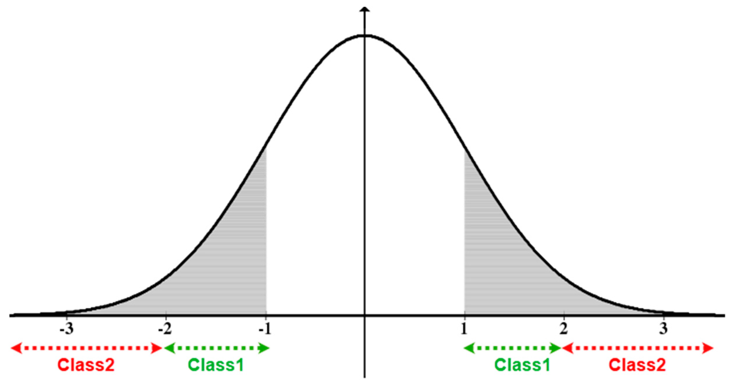
The central limit theorem defines both the parameters of the sampling distribution and the distribution of the sample means, based on the parameters of the initial population and the sample size. According to this, the means of independent samples from the same population $(\mathsf{\mu },\mathsf{\sigma }{}^2)$ follow a normal distribution of parameters $(\mathsf{\mu },\frac{{\mathsf{\sigma }}^2}{\mathrm{n}})$. A random variable Z follows the standard normal distribution (SND), denoted as $\mathrm{X}~\mathrm{N}(\mathsf{\mu },{\mathsf{\sigma }}^2)$ such that $\mathsf{\mu }=0\mathrm{and}\mathsf{\sigma }=1$. Then $\mathrm{Z}=\frac{\mathrm{X}-\mathsf{\mu }}{\mathsf{\sigma }}~\mathrm{N}(0,1).$ These formulas allow us to propose an alert classification system using an SND-based approach. Usually, medical samples from different people (patients) are used to create general medical rules (e.g., if x > y and t < mean => z is high). This probabilistic technique relies on the use of a sample that makes it possible to generate rules and therefore quantify common knowledge about all the patients. Our aim here was to use only patient-specific data and the behavior of vital variables to draw conclusions. We assumed that there were three classes of anomalies according to the severity of the observation. Therefore, the first class named Class 0 did not represent any health concern since it was squarely in a very close range to the normal and even ideal state of the mean values collected. The other two classes of generated alerts were Class 1 and Class 2 as:

• Class 0: with probability density $\mathrm{P}0\in \left[\mathsf{\mu }-\mathsf{\sigma },\mathsf{\mu }]\cup [\mathsf{\mu },\mathsf{\mu }+\mathsf{\sigma }\right]$;
• Class 1: with probability density $\mathrm{P}1\in \left[\mathsf{\mu }-2\mathsf{\sigma },\mathsf{\mu }-\mathsf{\sigma }]\cup [\mathsf{\mu }+\mathsf{\sigma },\mathsf{\mu }+2\mathsf{\sigma }\right]$;
• Class 2: with probability density $\mathrm{P}2\in \left[\mathsf{\mu }-4\mathsf{\sigma },\mathsf{\mu }-2\mathsf{\sigma }]\cup [\mathsf{\mu }+2\mathsf{\sigma },\mathsf{\mu }+4\mathsf{\sigma }\right]$.

These intervals were chosen based on the intrinsic nature of the normal distribution, namely the “68–95–99.7” rule. If the observation belongs to Class 1, an alert of Type 1 (Risky) is generated. Only the patient is therefore warned that these vital data are abnormal. Generally, observations of Class 1 were not critical, since the normal values were not far distant from the mean μ. If the observation belongs to Class 2 (critical), the system generates a Type 2 alert. Both the patient and the medical staff are thus warned that the patient is in an immediate danger, and requires an emergency intervention before its condition worsens, which can be fatal or have irreversible consequences for the patient’s health condition. Since this approach classifies the anomalies, it is essential to reiterate that observations that range in [μ − σ, μ + σ] do not represent a potential risk and are therefore not subject to this classification layer nor the previous classification layer using SVM. Figure 9 illustrates the generated classes (Class 1 and Class 2) of the standard normal distribution graph of a given data set. The x-axis represents the standard score of blood pressure values and the y-axis represents the corresponding probability density. As explained in this section, the generation of the Class 0 would not be taken into consideration throughout this work.

3. Results and Reports

3.1. Case Study: Blood Pressure

We distinguished between two different readings of BP, the systolic (S) and diastolic (D) values. We could also use the mean arterial pressure (MAP) as an intermediate value that represents S and D. In each simulation process, we generated multiple datasets representing different realistic medical cases.

Table 2. Overview of the international blood pressure standards.

Blood Pressure	Systolic (S)	Diastolic (D)	(MAP)
HBP (High Blood Pressure)	141 ≤ S	91 ≤ D	107 ≤ M
PHBP (Pre-High Blood Pressure)	121 ≤ S ≤ 140	81 ≤ D ≤ 90	94 ≤ M ≤ 106
IBP (Ideal Blood Pressure)	91 ≤ S ≤ 120	61 ≤ D ≤ 80	71 ≤ M93
LBP (Low Blood Pressure)	S ≤ 90	D ≤ 60	M 70

shows related medical rules and acronyms on which our study was based.

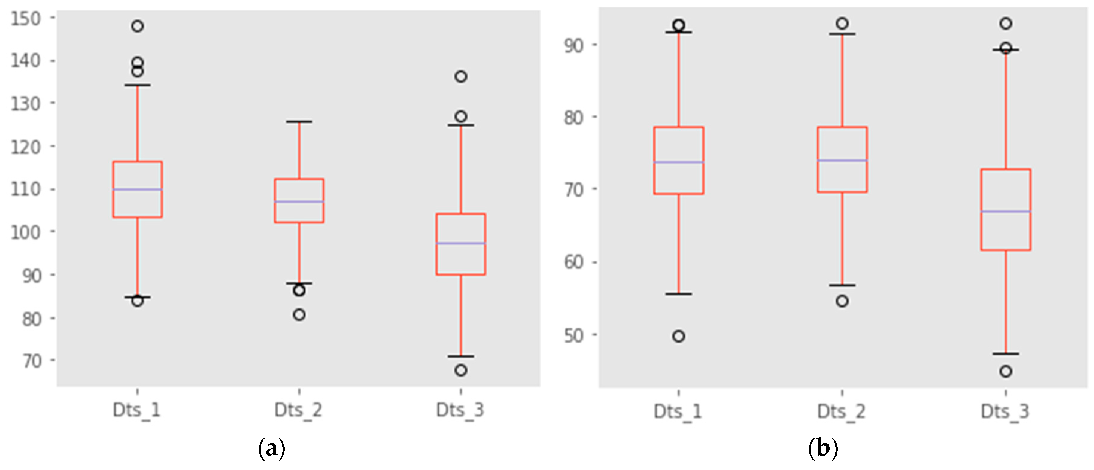
In order to apply the data processing described in this paper, three datasets for three different patients were generated, where μ_Sys, σ_Sys, μ_Dias and σ_Dias represent the mean of Systolic measures, standard deviation of Sys measures, mean of Diastolic measures and standard deviation of Dias measures respectively, as shown in

Table 3. Statistical summary of the generated datasets (Dts_i).

Datasets	$\mathsf{\mu }\_\mathbf{S}\mathbf{y}\mathbf{s}$	$\mathsf{\sigma }\_\mathbf{S}\mathbf{y}\mathbf{s}$	$\mathsf{\mu }\_\mathbf{D}\mathbf{i}\mathbf{a}\mathbf{s}$	$\mathsf{\sigma }\_\mathbf{D}\mathbf{i}\mathbf{a}\mathbf{s}$
Dts_1	110	10	73	6
Dts_2	107	7	74	7
Dts_3	98	11	67	8

. Since our data source structure was a transactional database, each Dts_i belonged to a time interval varying from ${\mathrm{T}}_{\mathrm{i}0}{\mathrm{to}\mathrm{T}}_{\mathrm{if}}$, where ‘i0′ and ‘if’ were the initial and final time entries of each dataset respectively.

These datasets were as follows:

• Dataset1 (Dts_1) corresponding to (Patient1): suffering from high blood pressure (HBP);
• Dataset1 (Dts_2) corresponding to (Patient2): suffering from pre-high blood pressure (PHBP);
• Dataset1 (Dts_3) corresponding to (Patient3): suffering from low blood pressure (LBP).

Figure 10 shows two box-plot representations of generated BP values. It gives a detailed view of the different values contained in our datasets.

3.2. Anomaly Detection Results

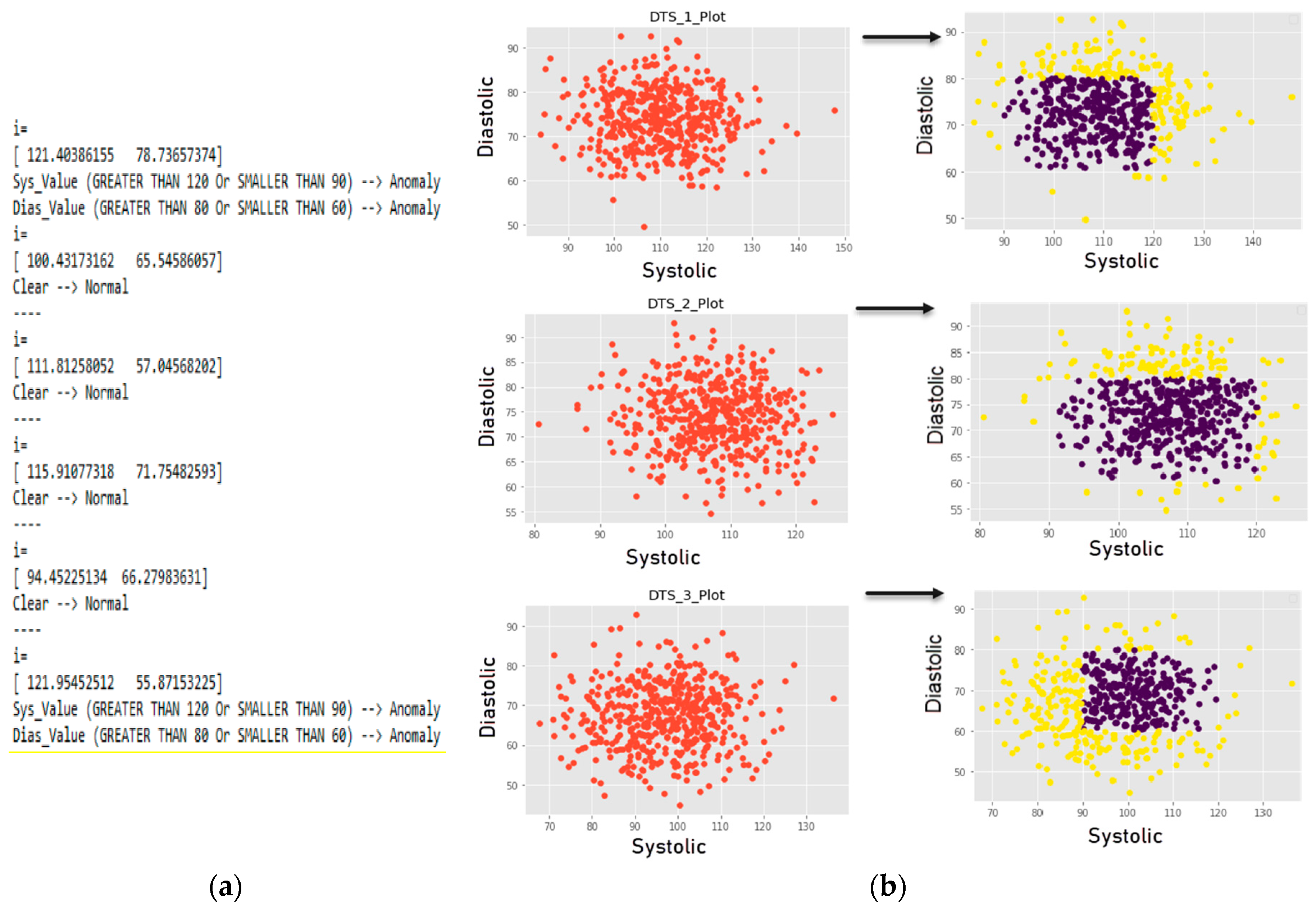
In this section, we applied the SVM classification algorithm. After obtaining a reliable classification model with adequate accuracy using SVM kernels, the algorithm was used to classify the sensed medical data from the WBAN device. We first randomly generated multiple datasets based on the rules presented above. For visualization of the decision function, we retained only two classes, making this a ‘binary classification problem’. The training datasets used ‘1′ as a decisional value for the ideal blood pressure (IBP) interval and ‘0′ for the HBP, PHBP and LBP intervals. This means that any value of systolic or diastolic BP that fell within the ideal BP range was a normal value; otherwise, the decisional value was considered as abnormal. The SVM model was using first the default values for the hyper parameters c and gamma. Then we tried different combinations to enhance the performance of the proposed classification model. Figure 11 shows the numerical method to classify the data according to medical rules, as well as the plot obtained for the different datasets. Blue and yellow colors represent normal and abnormal entries respectively. The datasets were sorted vertically from Dts_1 to Dts_3.

3.3. Classification Metrics

In order to validate a given model, it is required to estimate its performance using several metrics. In ML applications, learning from testing data is an essential step in approving the results obtained in the validation process. Overcoming unsatisfactory performance requires special attention to the detection of possible weaknesses related to overfitting and underfitting [27]. Throughout the rest of this paper, and in order to evaluate and then validate the performance of our approach, we would use several metrics as well as a confusion matrix that summarizes the rate of correct and incorrect predictions for our binary classification problem. The metrics were TP, FN, FP, TN and represent the number of true positives, false negatives, false positives and true negatives, respectively.

These four variables were defined as follows based on the confusion matrix:

• True positives (TP), where Class 1 is correctly predicted;
• True negatives (TN), where Class 1 is incorrectly predicted;
• False positives (FP), where Class 2 is incorrectly predicted;
• False negatives (FN), where Class 2 is correctly predicted.

These metrics would therefore allow us to calculate some common used standard performance measures such as accuracy, precision, F1-score and recall. The meaning of each measure was explained as follows:

• Accuracy—the overall performance of our model;
• Precision—the accuracy of the positive predictions;
• Recall—the coverage of the positive sample;
• F1-score—the harmonic average of the precision and recall.

Table 4. Confusion matrix.

	Class 0	Class 1
Class 0	TP	FP
Class 1	FP	FN

and

Table 5. Performance of classification model assessors.

Performance Measures	Formula
Accuracy	$\frac{\mathrm{TP}+\mathrm{TN}}{\mathrm{TP}+\mathrm{TN}+\mathrm{FP}+\mathrm{FN}}$
Precision	$\frac{\mathrm{TP}}{\mathrm{TP}+\mathrm{FP}}$
Recall	$\frac{\mathrm{TP}}{\mathrm{TP}+\mathrm{FN}}$
F1-score	$\frac{2\ast \mathrm{TP}}{2\ast \mathrm{TP}+\mathrm{FP}+\mathrm{FN}}$

show the detailed calculations of confusion matrix and standard performance as well as measures respectively for scores cited below.

3.4. Classification Performances

3.4.1. Initial Classification Results

In order to validate the results obtained, it is necessary to compare the classification results using SVM with other classification algorithms. Therefore, four of the most commonly used classifiers in the field of learning were chosen, namely: linear discriminant analysis, k-nearest neighbors, XGBoost and random forest. Precision, recall, f1-score and accuracy were the standard metrics (scores) provided to judge the performance of our approach. We mainly chose the K-nearest neighbors (KNN) because of its non-parametric nature since it allowed the classifier to react promptly to input changes in real time, noting that it did not rely on data from a particular domain or a particular distribution (normal distribution in our case). Since we also were working on a binary class model, the point clouds might be linearly separable in the representation space, choosing a linear separator such as the linear discriminant analysis (LDA) seemed to be adequate to our purpose. Based on a gradient boosting framework, XGBoost is a decision-tree-based classification algorithm that tends to outperform all machine learning algorithms when it comes to small and medium data. It uses several techniques such as parallel processing, tree-pruning and regularization to avoid overfitting. Another tree-based algorithm, named random forest (RF), was used during this comparison. RF can handle binary and numerical features with very low pre-processing, which needs to be done since data does not need to be rescaled or transformed. Therefore, comparing the results of our approach with those of XGBoost and RF would provide an excellent benchmark for the obtained performance. A set of experiments was conducted to provide a comparative study between these algorithms regarding their standard performances. This is shown in

Table 6. Comparative classification results using the standards performance.

Systolic	Classifier	Classes	Precision (%)	Recall (%)	F1-Score (%)
Dts_1	SVM (RBF)	Class 0	0.97	1	0.98
		Class 1	1	0.92	0.96
	LDA	Class 0	0.83	0.93	0.88
		Class 1	0.78	0.57	0.66
	KNN	Class 0	0.93	1	0.97
		Class 1	1	0.84	0.91
	XGBoost	Class 0	1	1	1
		Class 1	1	1	1
	RF	Class 0	1	1	1
		Class 1	1	1	1
Dts_2	SVM (RBF)	Class 0	0.97	0.99	0.98
		Class 1	0.97	0.9	0.93
	LDA	Class 0	0.88	1	0.94
		Class 1	1	0.56	0.72
	KNN	Class 0	0.96	0.99	0.98
		Class 1	0.97	0.87	0.92
	XGBoost	Class 0	1	1	1
		Class 1	1	1	1
	RF	Class 0	1	1	1
		Class 1	1	1	1
Dts_3	SVM (RBF)	Class 0	0.98	0.97	0.97
		Class 1	0.96	0.97	0.97
	LDA	Class 0	0.82	0.86	0.84
		Class 1	0.8	0.75	0.77
	KNN	Class 0	0.95	0.99	0.97
		Class 1	0.99	0.93	0.96
	XGBoost	Class 0	1	1	1
		Class 1	1	1	1
	RF	Class 0	1	1	1
		Class 1	1	1	1

.

The scores corresponding to classes 0 and 1 show the achieved results in classifying the data points in that particular class compared to the other one. The accuracy of the SVM (with RBF kernel) shows that the result obtained was very satisfactory given its values between 0.92 and 1 for all the standards. We could therefore conclude that our approach achieved the best performance for each dataset. In order to present a communicative result of our approach, it is also important to represent the calculations obtained during training and testing phases of learning.

Table 7. Training and testing results for the generated classifier.

Datasets	Classifier	Learning	Accuracy (%)
Dts_1	SVM (RBF)	Train	0.979
		Test	0.951
	LDA	Train	0.838
		Test	0.818
	KNN	Train	0.978
		Test	0.975
	XGBoost	Train	1
		Test	1
	RF	Train	1
		Test	1
Dts_2	SVM (RBF)	Train	0.991
		Test	0.969
	LDA	Train	0.898
		Test	0.896
	KNN	Train	0.985
		Test	0.963
	XGBoost	Train	1
		Test	1
	RF	Train	1
		Test	1
Dts_3	SVM (RBF)	Train	0.979
		Test	0.969
	LDA	Train	0.794
		Test	0.812
	KNN	Train	0.979
		Test	0.963
	XGBoost	Train	1
		Test	1
	RF	Train	1
		Test	1

illustrates the calculated accuracies of the three datasets. The related confusion matrices are represented in

Table 8. Confusion matrices of generated results using all classifiers.

Datasets		SVM (RBF)		LDA		KNN		XGBoost		RF
Dts_1		Class 0	Class 1	Class 0	Class 1	Class 0	Class 0	Class 1	Class 1	Class 1	Class 1
	Class 0	114	0	106	8	114	114	114	0	114	0
	Class 1	4	47	22	29	8	8	0	51	0	51
Dts_1		Class 0	Class 1	Class 0	Class 1	Class 0	Class 0	Class 1	Class 1	Class 1	Class 1
	Class 0	125	1	126	0	125	125	126	0	126	0
	Class 1	4	35	17	22	5	5	0	39	0	39
Dts_1		Class 0	Class 1	Class 0	Class 1	Class 0	Class 0	Class 1	Class 1	Class 1	Class 1
	Class 0	91	3	81	13	93	93	94	0	94	0
	Class 1	2	69	18	53	5	5	0	71	0	71

to support the results achieved.

3.4.2. Optimizing Results Using the Cross Validation Technique

Evaluating hyper-parameter (C and Gamma) requires special attention to detect potential ‘overfitting’ and ‘underfitting’ problems while gradually eliminating candidate learning models and finally ending up with a single optimal one. Otherwise, the obtained evaluation metrics will not reflect the performance of the generalization. Dividing each dataset into two sets (training/testing) or three sets (training/testing/validation) reduces significantly the number of samples that can be used to learn the model, and this will involve obtaining results depending on the sampling used during the training phase. To avoid this random data-related dependency, applying the cross-validation technique was proven to be the solution. In order to reduce to a minimum, the low efficiency associated with randomly splitting training and testing data set, scientists are likely to use the K-fold approach. In this technique, each of the datasets was randomly divided into k subsets of the same scale. Then we tested the shaped classification models k times. The final representative accuracy was calculated as the average of the k precision measurements. Finally, the overall accuracy was calculated as the average of the k accuracies. As detailed in Section 3.3, it was essential to apply a cross validation on our model in order to overcome the problems associated with learning to finally obtain a reliable and generalized model for the entire sample. We had chosen to divide each dataset into five (k = 5) components, and then calculated the accuracy of each part to finally return their average score.

Table 9. Cross validation accuracies calculations.

	A1	A2	A3	A4	A5	Average (%)
Dts_1	1.00	1.00	1.00	1.00	1.00	1.00 ± (0.00)
Dts_2	1.00	0.99	1.00	1.00	1.00	0.99 ± (0.01)
Dts_3	1.00	1.00	1.00	0.98	1.00	0.99 ± (0.01)

summarizes the obtained calculations as well as their average. This value was representative of the dataset and would be retained for later usage. A1, A2, A3, A4 and A5 represented the calculated accuracies of each cross validation split.

These scores were done using the optimal C and Gamma parameters, which values are represented in

Table 10. Optimized C and Gamma parameters for the radial basis function (RBF)-kernel.

Datasets	C	Gamma (γ)
Dts_1	10.1	0.01
Dts_2	20.2	0.01
Dts_3	40.4	0.01

. Accuracies A1, A3 and A5 of the SVM classifier applied to all datasets with optimized parameters (C and Gamma) were therefore equal to 1 (100%). So, our model was as efficient as those XGBoost and RF, which accuracies were also equal to 1.

3.5. Testing to Assess the Normality of Distribution

Before applying the proposed probabilistic approach to the generated samples, we first needed to test whether our datasets fitted a normal distribution. We, therefore, needed to determine that there were no grounds to reject the null hypothesis, which stated that the data was normally distributed. To do so, several statistical tests could be applied. If the results were positive (greater than 0.05 for some and less than 0.05 for others), a probability graph was plotted to validate the hypothesis; otherwise, the use of a distributive approach could not be justified and must be rejected.

3.5.1. Normality Test Using Statistical Metrics

It is worth recalling that this process focused on data that fit the normal distribution. Otherwise, the first layer classification using SVM is sufficient to detect whether a medical entry is safe or considered as an anomaly. Therefore, in this case, the conclusions drawn during the 2nd classification layer did not hold.

The statistical algorithms listed below are efficient testing methods that return two measures: numerical values representing decision results called the p-value and s-value, which is equivalent to the critical statistical value of our distributions.

• Anderson–Darling (AD);
• Shapiro–Wilk (SW);
• Kolmogorov–Smirnov (KS);
• D’Agostino and Pearson (DP);

We applied all four of these algorithms in order to rule out the possibility that our data does not follow a normal distribution.

Table 11. Results of normality tests using statistical metrics.

Systolic	Normality Test	S-Value	p-Value	Result
Dts_1	AD	0.299	0.781	√
	SW	0.996	0.284	√
	KS	1.0	0.0	√
	DP	2.653	0.26	√
Dts_2	AD	0.221	0.781	√
	SW	0.996	0.274	√
	KS	1.0	0.0	√
	DP	3.324	0.19	√
Dts_3	AD	0.492	0.781	√
	SW	0.996	0.339	√
	KS	1.0	0.0	√
	DP	0.035	0.983	√
Diastolic	Normality Test	S-Value	p-Value	Result
Dts_1	AD	0.274	0.781	√
	SW	0.998	0.676	√
	KS	1.0	0.0	√
	DP	0.056	0.972	√
Dts_2	AD	0.166	0.781	√
	SW	0.998	0.923	√
	KS	1.0	0.0	√
	DP	0.835	0.659	√
Dts_3	AD	0.29	0.781	√
	SW	0.998	0.668	√
	KS	1.0	0.0	√
	DP	0.818	0.664	√

shows the results of testing of the patient samples.

The results obtained from the normality test using AD, KS, SW and DP showed that there were no grounds to reject the null hypothesis that the data were normally distributed. The p-values returned by each statistical test could be interpreted as follows: Anderson–Darling (AD), Shapiro–Wilk (SW) and D’Agostino and Pearson (DP) must return a p-value greater than 0.05, while Kolmogorov–Smirnov (KS) must return a p-value smaller than 0.05. These were the standards that the p-value of each test must meet in order to validate our hypothesis.

As can be seen from the table above, all four of the normality tests results show that our datasets fitted a normal distribution; the s-values and p-values indicate statistical significance and met the confirmation intervals

3.5.2. Normality Test Using a Quantile–Quantile Probability Plot

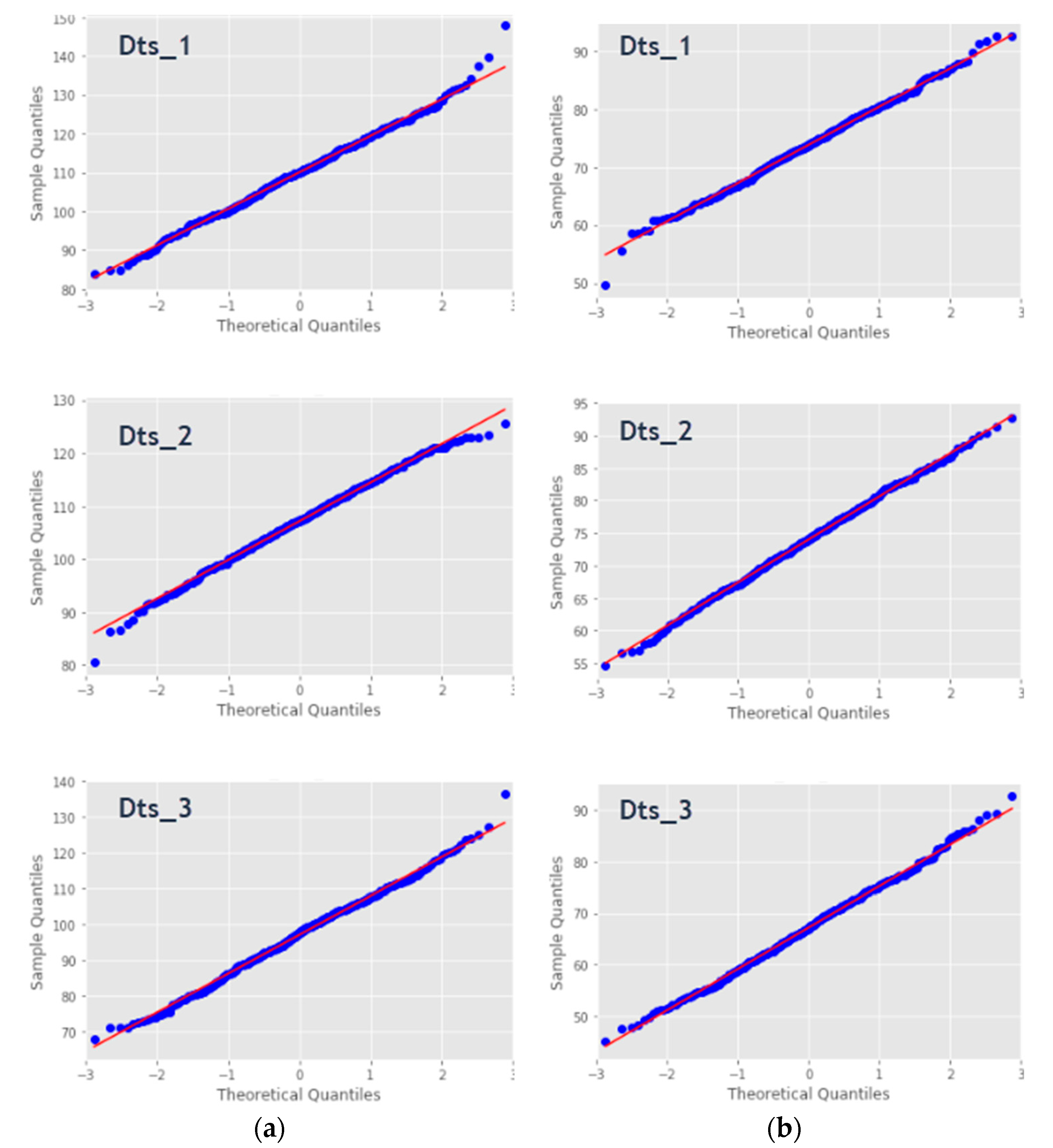
A Quantile–Quantile (Q–Q) is a graphical probability plot method that compares two probability distributions by plotting their quantiles against each other. This approach displays the observed values against normally distributed data, represented by the red line. Normally distributed data are represented by blue dots and fall along this line. Figure 12 illustrates the Q–Q plots applied to the sample used in the statistical test. It can explicitly show the closeness of the data points, thus describing the linearity of the normally distributed sample. We could also see the outliers that could probably be represented during the second classification phase. The theoretical distribution is the normal distribution with mean 0 and standard deviation 1.

The results obtained from the normality test using the Q–Q plot show that there were no grounds to reject the null hypothesis that the data were normally distributed, a conclusion that agreed with that obtained using the AD, KS, SW and DP statistical tests.

3.6. Applying the Normal Distribution to the Generated Samples

The section entitled “Testing to assess the normality of distribution” demonstrated the possibility of applying the normal distribution, which led us to illustrate our approach in the following paragraphs. We could calculate the probabilities that a variable has a value that is less than, equal to or greater than a specific critical value with respect to outliers, means or other thresholds. To do this, we transformed data from a normal distribution, where X~N(μ, σ), to a standard normal distribution, where X~N(0, 1). This allowed us to use the SND probabilistic approach. These calculations could help medical staff (doctors) to generate information and diagnoses as well as enriching and enhancing the medical history of a patient. It could also help to measure the efficiency and progress of an applied treatment. Using the same sample as in the previous sections, the following results could represent the evolution of a patient’s state of health. Figure 13 provides an explanation of the idea behind this process by illustrating all the Sys and Dias measures of our datasets in the box-plot form, side by side with the representation of their respective normal distributions. The orange-colored area is the one covered by this classification, which represents a real danger to our patients. The present readings were not normalized X~N(μ, σ) for a meaningful illustration of the BP actual values.

Table 12. Results of anomalies calculations.

Probabilistic Analysis	Class_1_Sys	Class_2_Sys	Class_1_Dias	Class_2_Dias
Patient 1 (Pre-high BP)	62	20	59	31
Patient 2 (high BP)	8	18	71	17
Patient 3 (Low BP)	73	26	88	19

summarizes the achieved results during this phase. The reduction in the number of anomalies clearly demonstrated the effectiveness of our classification approach after the first process using SVM. Note that Class 1 had a probability P1 ∈ [μ – 2σ, μ – σ] ∪ [μ + σ, μ + 2σ] and Class 2 a probability P2 ∈ [μ – k*σ, μ – 2σ] ∪ [μ + 2σ, μ + k*σ]/k $\ge$ 3, which means that the more an anomaly was distant from the mean of the sample, the riskier it was deemed to be.

3.6.1. Integrating Knowledge Based on the Normal Distribution

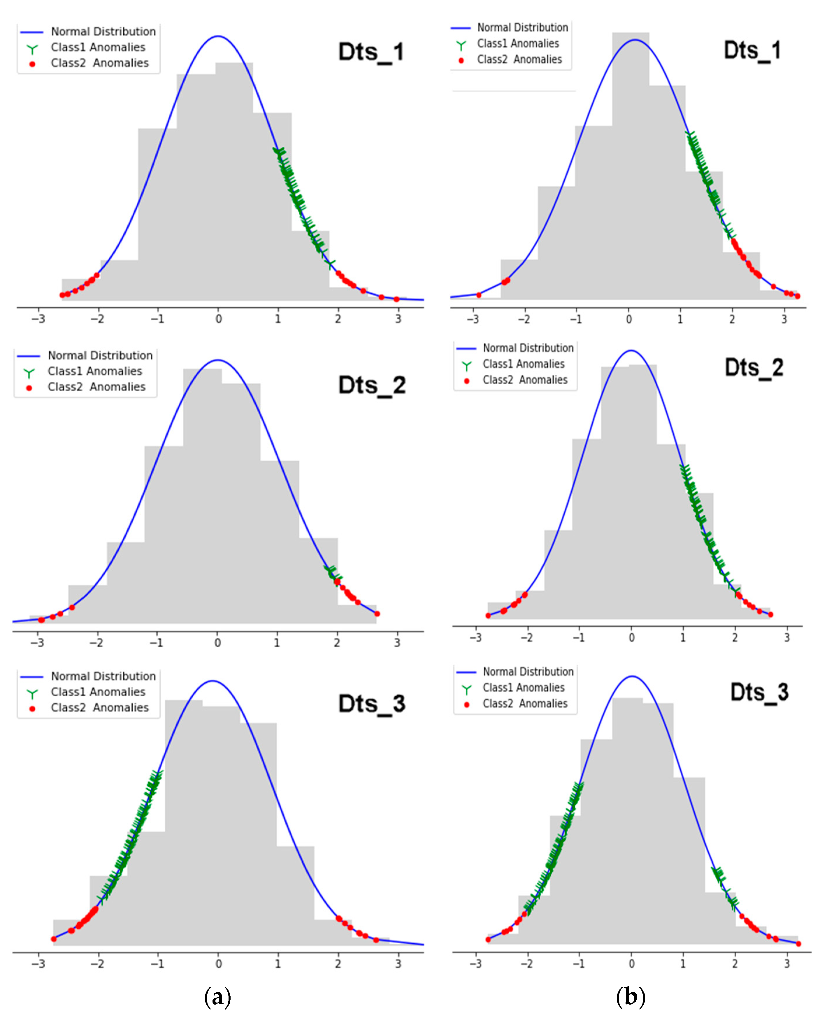
According to the results shown in Figure 14, we clearly distinguished the different metrics that represent the abnormal values. The green (Y) and the red crosses (dots) represent the detected values belonging to Class 1 and Class 2 respectively. Thus, given a new entry, the system would automatically issue alerts according to the classifications model made of the recorded values. Since this approach classified the anomalies, it was essential to reiterate that observations with probabilities that ranged in [μ − σ, μ + σ] did not show any threat and were therefore subject to neither this classification process nor the previous process using SVM.

As explained in this paper, values belonging to Class 1 did not represent an immediate danger. This involves detecting several anomalies by using SVM first, then classifying the returned abnormal values and issuing the corresponding alerts according to their dangerousness. The third plot of Figure 14 corresponding to panel (b), unlike all other plots in which we noticed the presence of Class 1 anomalies either to the right or to the left of the mean, represents an interesting case, since most of its parameters and statistical values belonged to the abnormal blood pressure that ranged in [–3, –1] and some measures belonging to both classes that ranged in [1, 3] for diastolic records. This is due to the fluctuation of data around the corresponding means. The approach supported by these representations therefore returned a very satisfactory result since we had chosen datasets from which patients suffered from BPH, PHBP and LBP respectively for Dts_1, Dts_2 and Dts_3. As explained in Table 2, HBP and PHBP measures generally represented anomalies that were strongly present to the right of the mean, unlike LBP where anomalies were displayed to the right of the mean. This enabled us to pinpoint the areas that were a threat to the patient’s health.

3.6.2. Final Learning Model Results

This process took as an input the data that had already underwent a first classification of anomalies according to the rules presented in Table 2. Then came the step where we applied our normal distribution based approach to distinguish the anomalies detected according to their severity. This allowed us to retain only the data representing an abnormal measurement and thus keeping the same properties of our classifier (which parameters were optimized to achieve the best results in term of accuracy in the previous processes). We also re-trained our classifier so that it could learn to picture new entries in order to generate alerts according to their dangerousness (‘Risky’ for Class 1 and ‘Critical’ for Class 2). The results of this final classification are depicted in

Table 13. Cross validation accuracies calculations using the final classifier.

Datasets	A1	A2	A3	A4	A5	Average (%)
Dts_1	1.00	1.00	1.00	0.98	0.99	0.99 ± (0.01)
Dts_2	1.00	0.98	0.98	1.00	1.00	0.99 ± (0.01)
Dts_3	1.00	1.00	1.00	1.00	1.00	1.00 ± (0.00)

and

Table 14. Optimized C and Gamma parameters for the RBF-kernel.

Datasets	C	Gamma (γ)
Dts_1	20.2	0.01
Dts_2	20.2	0.02
Dts_3	50.5	0.01

.

4. Discussion

The initial number of collected values was 500 for each dataset. During the first phase of classification using SVM, an anomaly detection ratio of 68.2%, 75.4% and 55.2% was observed correspondingly for Dts_1, Dts_2 and Dts_3. Comparing these results with the other two classifiers, namely linear discrimination (LD) and k-nearest neighbors (KNN), it could be seen that SVM achieved the best scores. We considered an anomaly, the Tuple {Sys,Dias}, one or both metrics presenting a value not belonging to the IBP standard mentioned in Table 2. As a result, critical values were further penalized, providing a very realistic reading that did not neglect any data that could represent a danger.

Table 15. Summary of the achieved results and ratios associated to initial data.

Results	Dts_1	Dts_2	Dts_3
Initial Length	500 (100%)	500 (100%)	500 (100%)
Normal Measures	159 (31.8%)	123 (24.6%)	224 (44.8%)
Anomalies (SVM)	341 (68.2%)	377 (75.4%)	276 (55.2%)
Anomalies (Normal Distribution)	149 (29.8%)	120 (24%)	224 (44.8%)

epitomizes the results obtained and the calculated ratios.

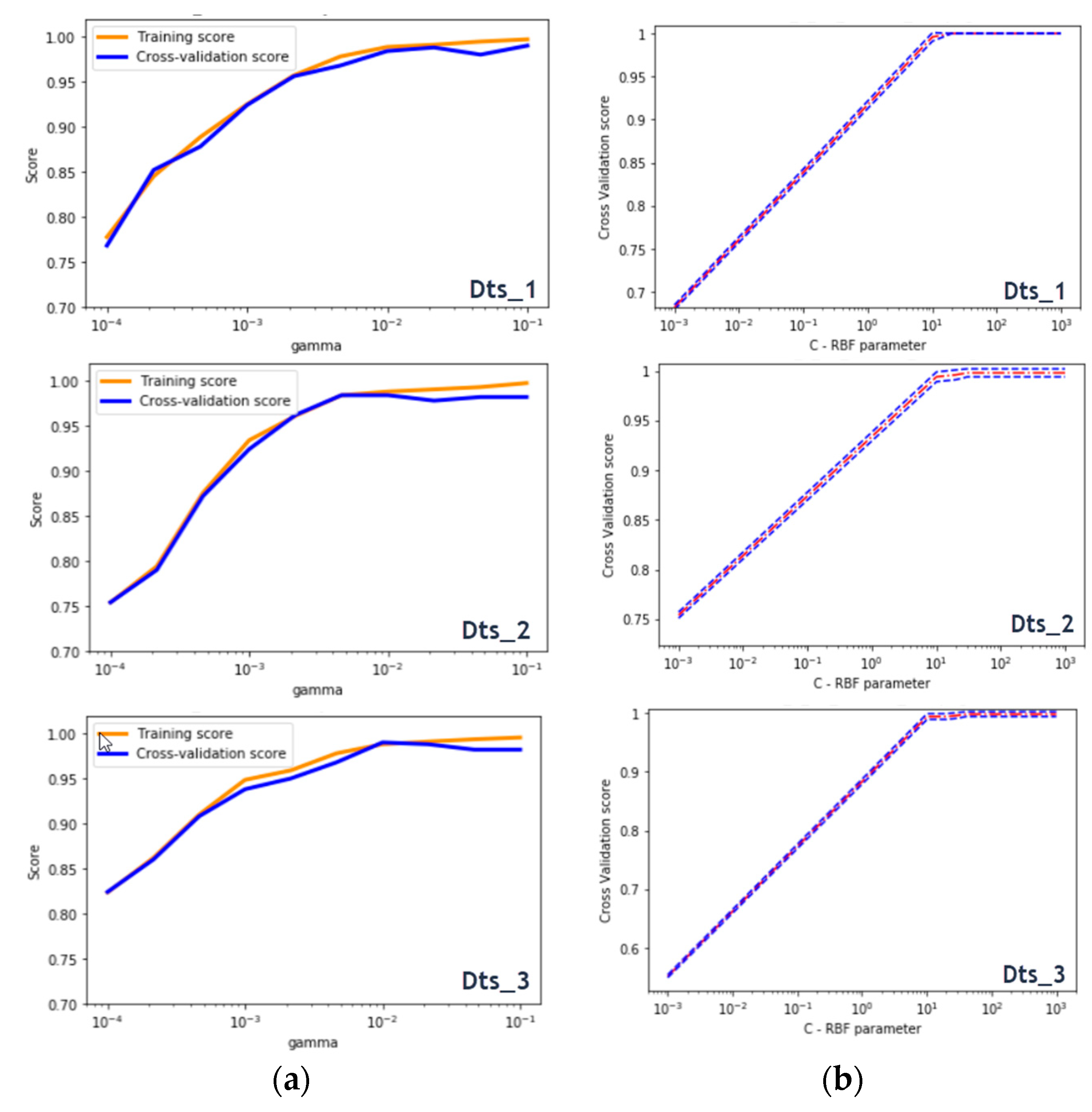
During the optimization phase of the SVM classifier parameters, the representative curves of the different data sets appeared to have the same behavior. The higher the C-axis value, the better the cross-validation score was, up to a certain constant value when it reached a steady-state score. It is worth noting that a large C resulted in a low bias and a high variance. This explained why the system significantly penalized the cost of misclassification by allowing the model to freely select more samples as support vectors. Otherwise, a small C led to a higher bias and a lower variance, this affected the decision surface to be smoother. For the three datasets, the C values ranged in [10.1, 40.4]. Initially, the gamma parameter specified the scale of influence of a single learning example. The higher the gamma value was, the more it tried to adjust accurately to the training data set. For the three datasets, γ = 0.01. Mainly, increasing the values of C and γ might lead to overfitting the training data. During this critical learning process, both parameters were used to evaluate the performance of our system by comparing the training results with those of the cross validation scores. As mentioned above, the RBF-kernel based support vector machine returned the best results. This was illustrated using the confusion matrix as well as some metrics such as precision, recall, f1-score and accuracy. The plots in Figure 15 show that the training and validation scores increased to a certain point of stability with recorded slight differences. It was a sign of under-fitting. Then, the classifier operated properly for medium and high gamma levels.

Note that before the optimization phase, accuracies ranged in [0.95, 0.99] (for SVM). Thus, it was effective in preserving our analysis from overfitting or/and underfitting to divide our test learning data into k = 5 folds. Using this process, the three datasets responded positively by returning results that far exceeded the decision thresholds and that we believed were ideal. In this study, we set a minimum accuracy threshold of 80%. Therefore, metric scores above this value were retained. This collection was largely exceeded since it sometimes reached a perfect score of 1 (100%) essentially when the k-fold based cross-validation was used to validate our study.

Before being able to apply our normal distribution approach, it was essential to justify this step by testing whether our data allowed the use of this probabilistic solution. This was proven by using two different and complementary techniques, the Q–Q plot and the statistical test. In the Q–Q plot case, and by considering the sorted sample values on the y-axis as well as the expected quantiles on the x-axis, we could identify from the way in which the values in some sections of the graph did not approach the linear representation locally, whether they were more or less correlated than the theoretical distribution. The technique yielded quite similar representations since the distribution was the same (normal), but the observations took a symmetrical form so that no bias was observed (the mean was equal to or close to the median). Almost all the points fell into the straight line, with some observations that curved slightly in the extremities. This could be a sign of a light-tailed behavior since the sample grew slower than the normal distribution, approximately from (–3,–2) and reached its highest quantile before the standard normal distribution from (2,3). Thus, all the achieved results in this regard had proven our approach to be right. For the second test, it was required to use different statistical algorithms to support our assessment. This was done using four methods, namely: Anderson–Darling (AD), Shapiro–Wilk (SW), Kolmogorov–Smirnov (KS) and D’Agostino and Pearson (DP). The obtained results fit perfectly the standards depicted in Table 11, as all the p-values were higher than 0.05 for AD, KS and DP, and were lower than 0.05 for KS. By demonstrating in two different ways that our data provided an ideal basis for normal distribution enforcement, this process was successfully achieved.

In order to clearly define our approach, an explanatory graphic representation was developed. This concerns Figure 13, where the most important data form was illustrated, namely: boxplot, histogram as well as the plotted normal distribution. In the latter we represented exactly the area likely to be dangerous to our patient, and whose metrics (highlighted in orange) exceeded the set threshold. During binary classification of the dangerousness of these anomalies using the normal distribution, the following ratios were noted: 43.7%, 31.8% and 81.1% respectively for Dts_1, Dts_2 and Dts_3.

Table 16. Summary of the achieved results and ratios associated to the abnormal data.

Results	Dts_1	Dts_2	Dts_3
Anomalies	341 (100%)	377 (100%)	276 (100%)
Anomalies (Normal Distribution)	149 (43.7%)	120 (31.8%)	224 (81.1%)

summarizes the obtained calculations and ratios.

As indicated in this process, two classes were taken into account. This number might vary according to the distance σ separating a value at the average μ from the sample of anomalies. This considerably reduced the number of anomalies to keep only those most likely to cause a more or less life-threatening factor for the patient. Looking closely at the results obtained in Table 13, it could be seen that the number of Class 1 anomalies was greater than the one of class 2. This was due to the intrinsic nature of this distribution, since the more distant σ from the mean μ deviated, the more the number of values decreased. This justified the different results obtained. It should be mentioned that it was normal to produce results where no anomalies belonging to Class 1 were represented to the left of μ or/and to the right of μ. This was on the grounds that the values within this area did not represent a danger since they had previously been classified as normal and ranged in [90, 120] and [60, 80] for Sys and Dias measures respectively. With this in view, the number of data undergoing this classification was quite small compared to the original dataset since it was overlooked in this section, applying a classification of anomalies and then retaining only those that represent a real health risk for our patients. This considerably reduced the final number of readings we investigated. We also considered important and complementary to calculate the required time for this classification and for the previous one.

Table 17. Summary of the achieved time results for all binary classifiers.

Phases	Classifiers	Dts_1	Dts_2	Dts_3
Phase 1	SVM	0.001 s	0.003 s	0.003 s
	KNN	0.002 s	0.003 s	0.002 s
	LDA	0.004 s	0.004 s	0.003 s
	XGBoost	1.972 s	0.92 s	1.00 s
	Random Forest	0.013 s	0.011 s	0.011 s
Phase 2	SVM	0.0019 s	0.002 s	0.001 s
	KNN	0.0019 s	0.002 s	0.0019 s
	LDA	0.0049 s	0.002 s	0.002 s
	XGBoost	1.09 s	0.912 s	0.91 s
	Random Forest	0.011 s	0.011 s	0.011 s

shows the fit time for normalized parameters during the classification technique process. A time optimization was done for all the datasets by scaling data between 0 and 1.

In terms of time complexity, it was clear that the performance was rather favorable for the SVM, LDA and KNN algorithms since their processing times did not exceed 0.04 s, in contrast to XGBoost and random forest, which returned perfect results, but in a significant time, sometimes of around 1.97 and 0.01 s respectively. While using XGBoost, training data generally took longer because trees were built sequentially. We could therefore conclude that our SVM-based approach returned very satisfactory classification results, and this, in a very short processing time compared to the other algorithms. The accuracy was equal to or slightly less than 1 (100%) while the time did not exceed 0.003 s. This led us to conclude that these scores therefore validated the performance results of this approach. It was also important to introduce a comparison with a multi-class classifier (number of classes >2). This was done using SVM, but this time defining three classes instead of two, called safe (S), risky (R) and critical (C). The Class 0 data returned by the first classification layer using SVM were classified as S, while data that belonged to Class 1 and Class 2 when normal distribution was applied were classified as S and C respectively. The results obtained during this multi-classification process are illustrated in

Table 18. Training and testing results for multi-class SVM.

Datasets	Learning	Accuracy (%)
Dts_1	Train	0.743
	Test	0.757
Dts_2	Train	0.722
	Test	0.757
Dts_3	Train	0.871
	Test	0.878

while

Table 19. Training and testing results for multi-class SVM.

Classifier	Dts_1	Dts_2	Dts_3
Multi-class SVM	0.003 s	0.002 s	0.001 s

shows its time duration.

Based on the results of Table 18, we note that this method returned average training and testing accuracies that were less than 0.76 for the first two datasets. While it returned scores higher than 0.87 for Dts_3, which was acceptable based on our pre-set threshold of 80%. Regarding the processing time, it seemed clear that this approach did not exceed 0.003 s for each of the three datasets, which was still a very good time compared to those obtained using XGBoost and RF. These comparisons made between our 2-layer classification approach, using SVM as well as the normal distribution, and those using first, the powerful tree-based classifiers XGBoost and RF, and then the multi-class SVM classifier, have shown that our approach was getting near perfect scores while maintaining a very low processing time.

Table 20. Simulation of the manipulations carried out using several measurements.

Tuple	Values	Decision	Normalization	Mean	Std	Class	Alert
{123.19, 78.63}	123.19	Abnormal	1.67	110	10	1	{Sys,Dias} ∈ Class 1
	78.63	Normal	-	73	6	-	High risk
{93.02, 67.65}	93.02	Normal	-	110	10	-	No risk
	67.65	Normal	-	73	6	-
{107.87, 84.57}	107.87	Abnormal	-	107	7	-	{Sys,Dias} ∈ Class 1
	84.57	Normal	1.51	74	7	1	High risk
{108.77, 59.66}	108.77	Normal	-	107	7	-	{Sys,Dias} ∈ Class 2
	59.66	Abnormal	−2.04	74	7	2	High risk
{110.73, 67.70}	110.73	Normal	-	98	11	-	No risk
	67.70	Normal	-	67	8	-
{75.53, 55.49}	75.53	Abnormal	−2.04	98	11	2	{Sys,Dias} ∈ Class 2
	55.49	Abnormal	−1.43	67	8	1	Critical risk

illustrates a use example of this intelligent system. Several measurements of different values were taken as inputs in the tuple form {Sys, Dias}, then the treatments performed based on our approach were carried out.

As indicated in the description of our approach, if one of the measurements of the tuple {Sys, Dias} represented an anomaly, then the entire tuple was considered to be a danger to the patient. Mean and Std represent the mean and standard deviation of the sample from which the measurements were taken. The tuples {93.02, 67.65} and {110.73, 67.70} returned a negative risk alert since they both belonged to the IBP. So, there was no need to implement the process. The tuple {123.19, 78.63} returned a high risk alert because of its Sys value that belonged to Class 1. Finally, the tuple {75.53, 55.49} returned a critical risk alert given that both Sys and Dias values belonged to Class 2 and Class 1 respectively and therefore the tuple would be considered as a Class 2 alert according to the rules underlying our approach, which automatically classified the tuple in the highest class of the two child classes.

Table 21. Risk classification truth table.

Җ	S	R	C
S	-	C1	C2
R	C1	C1	C2
C	C2	C2	C2

depicts those rules based on our introduced logical operator Җ where S, R and C represent normal, Class 1 and Class 2 respectively.

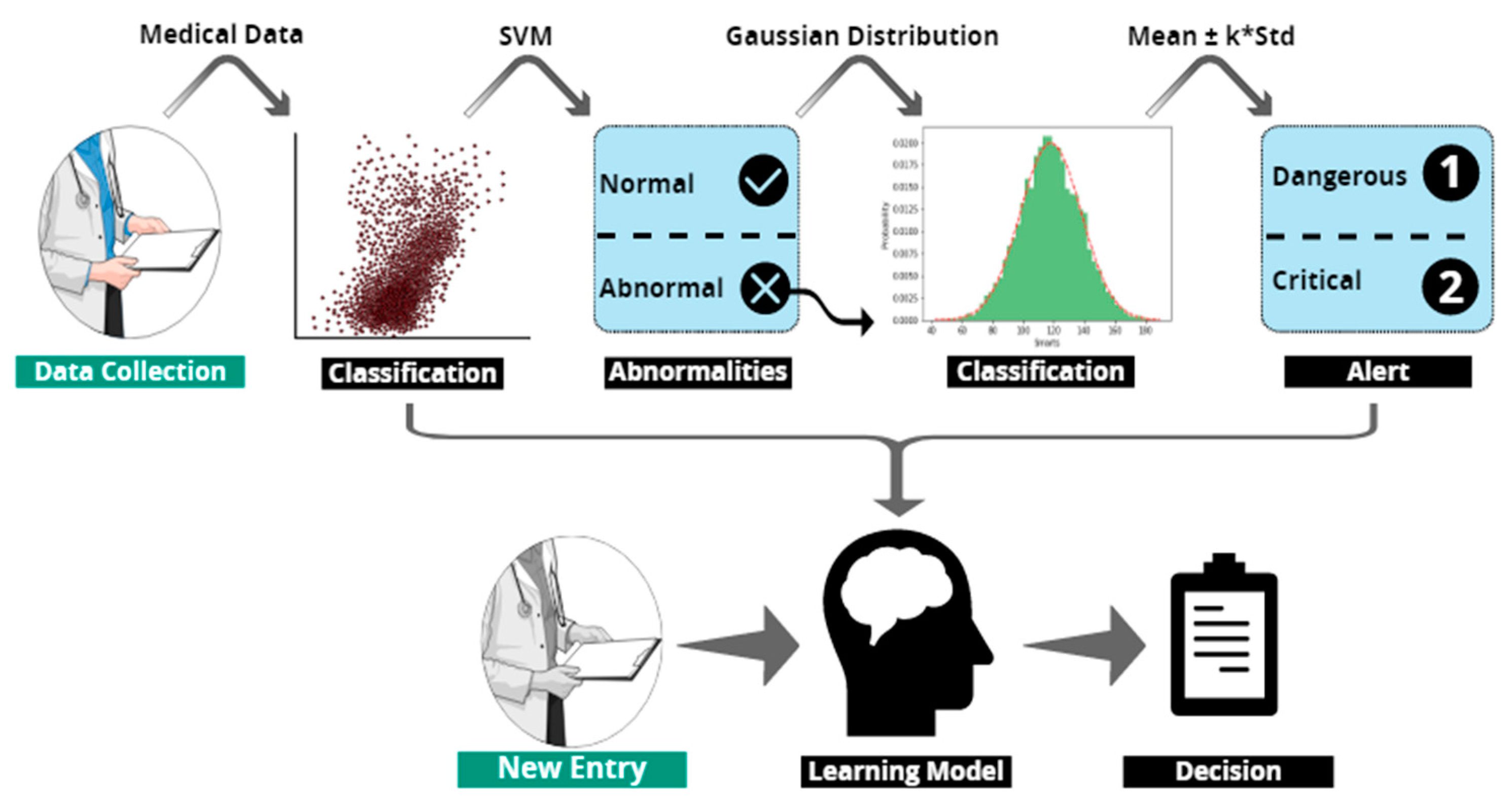
Figure 16 summarizes our approach from data collection, through the discovery of the learning model based on the two classification processes, to the final model used to precisely classify any abnormality that might present a high or a critical risk for the patient.

So, this research work responded perfectly to our concern about proposing an intelligent system that was specific to each patient and about avoiding knowledge based on generalized thresholds. That being said, our study offered a detection learning model adapted to a single patient on a case-by-case basis. Future works will focus on modeling processes using techniques to optimize the active search for intervals and boundary zones related to the achieved results using the normal distribution. This would allow a deeper learning of the patient’s habits and thus adapt a given medical treatment.

5. Conclusions

Ubiquitous healthcare systems have attracted a great deal of attention in recent years for their application in numerous fields such as e-health, telemedicine and home nursing. The enormous amount of research in this area motivates us to present this work. In this paper, a smart ubiquitous healthcare monitoring architecture was developed that was capable of handling the healthcare process from the gathering of bio-sensed data to the management of critical information for effective administration of healthcare monitoring in order to provide services. In this study, we used WBAN sensors to gather vital patient information, and then transmitted this information to be separated into different dataset categories. Statistical calculations were carried out with the aim of efficiently classifying abnormal physiological values (blood pressure application). Taken together, these results provided additional evidence that ubiquitous smart systems could be efficiently applied to the Internet of Things with the use of smart technologies that were capable of communicating medical data to be analyzed. The results of this work appeared to validate the proposed model. This study was not specifically designed to evaluate factors related to security or scalability, or to provide data that are missing due to gathering and communication issues. One of the major drawbacks of this work was that of finding medical data sources that naturally fit a probabilistic approach. Blood pressure readings are known to fit this hypothesis, and this was confirmed using various normality tests as described above. Future work will focus on combining learning techniques with a software-defined networking system while focusing on data behavior in critical boundaries related to the application of the normal distribution to generate new insights.

References

1. Qadri, S.F.; Awan, S.A.; Amjad, M.; Anwar, M.; Shehzad, S. Applications, challenges, security of wireless body area networks (WBANs) and functionality of IEEE 802.15. 4/ZIGBEE. Sci. Int. 2013, 25, 697–702. [Google Scholar]
2. Movassaghi, S.; Abolhasan, M.; Lipman, J.; Smith, D. Wireless body area networks: A survey. IEEE Commun. Surv. Tutor. 2014, 16, 1658–1686. [Google Scholar] [CrossRef]
3. Cesarini, D.; Calvaresi, D.; Marinoni, M.; Buonocunto, P.; Buttazzo, G. Simplifying tele-rehabilitation devices for their practical use in non-clinical environments. In Proceedings of the International Work-Conference on Bioinformatics and Biomedical Engineering, Granada, Spain, 15–17 April 2015; pp. 479–490. [Google Scholar] [CrossRef]
4. Shi, X.; An, X.; Zhao, Q.; Liu, H.; Xia, L.; Sun, X.; Guo, Y. State-of-the-Art Internet of Things in Protected Agriculture. Sensors 2019, 19, 1833. [Google Scholar] [CrossRef] [PubMed]
5. Ou, Y.Y.; Shih, P.Y.; Chin, Y.H.; Kuan, T.W.; Wang, J.F.; Shih, S.H. Framework of ubiquitous healthcare system based on cloud computing for elderly living. In Proceedings of the APSIPA Annual Summit and Conference, Kaohsiung, Taiwan, 29 October–1 November 2013; pp. 1–4. [Google Scholar] [CrossRef]
6. Calvaresi, D.; Cesarini, D.; Sernani, P.; Marinoni, M.; Dragoni, A.F.; Sturm, A. Exploring the ambient assisted living domain: A systematic review. J. Ambient Intell. Humaniz. Comput. 2017, 8, 239–257. [Google Scholar] [CrossRef]
7. McPake, B.; Mahal, A. Addressing the needs of an aging population in the health system: The Australian Case. Health Syst. Reform 2017, 3, 236–247. [Google Scholar] [CrossRef] [PubMed]
8. Wang, H.; Choi, H.S.; Agoulmine, N.; Deen, M.J.; Hong, J.W.K. Information-based sensor tasking wireless body area networks in U-health systems. In Proceedings of the 2010 International Conference on Network and Service Management (CNSM), Niagara Falls, ON, Canada, 25–29 October 2010; pp. 517–522. [Google Scholar] [CrossRef]
9. Saggio, G.; Cavallo, P.; Bianchi, L.; Quitadamo, L.R.; Giannini, F. UML model applied as a useful tool for Wireless Body Area Networks. In Proceedings of the International Conference on Wireless Communication, Vehicular Technology, Information Theory and Aerospace & Electronic Systems Technology, Aalborg, Denmark, 17–20 May 2009; pp. 679–683. [Google Scholar] [CrossRef]
10. Burges, C.J. A tutorial on support vector machines for pattern recognition. Data Min. Knowl. Discov. 1998, 2, 121–167. [Google Scholar] [CrossRef]
11. Islam, M.S.; Islam, M.T.; Almutairi, A.F.; Beng, G.K.; Misran, N.; Amin, N. Monitoring of the Human Body Signal through the Internet of Things (IoT) Based LoRa Wireless Network System. Appl. Sci. 2019, 9, 1884. [Google Scholar] [CrossRef]
12. Smail, O.; Kerrar, A.; Zetili, Y.; Cousin, B. ESR: Energy aware and Stable Routing protocol for WBAN networks. In Proceedings of the 12th International Wireless Communications & Mobile Computing Conference (IWCMC 2016), Paphos, Cyprus, 5–9 September 2016; pp. 452–457. [Google Scholar] [CrossRef]
13. Jung, J.; Ha, K.; Lee, J.; Kim, Y.; Kim, D. Wireless body area network in a ubiquitous healthcare system for physiological signal monitoring and health consulting. Int. J. Signal Process. Image Process. Pattern Recognit. 2008, 1, 47–54. [Google Scholar]
14. Jovanov, E.; Milenkovic, A.; Otto, C.; De Groen, P.C. A wireless body area network of intelligent motion sensors for computer assisted physical rehabilitation. J. Neuroeng. Rehabil. 2005, 2, 6. [Google Scholar] [CrossRef] [PubMed]
15. Chen, W.; Hu, J.; Bouwstra, S.; Oetomo, S.B.; Feijs, L. Sensor integration for perinatology research. Int. J. Sens. Netw. 2011, 9, 38–49. [Google Scholar] [CrossRef]
16. Kang, J.S.; Jang, G.; Lee, M. Stress status classification based on EEG signals. J. Inst. Internet Broadcast. Commun. 2016, 16, 103–108. [Google Scholar] [CrossRef]
17. Kim, J.; So, J.; Choi, W.; Kim, K.H. Development of a mobile healthcare application based on tongue diagnosis. J. Inst. Internet Broadcast. Commun. 2016, 16, 65–72. [Google Scholar]
18. Kumar, V.; Gupta, B.; Ramakuri, S.K. Wireless body area networks towards empowering real-time healthcare monitoring: A survey. Int. J. Sens. Netw. 2016, 22, 177–187. [Google Scholar] [CrossRef]
19. Hanen, J.; Kechaou, Z.; Ayed, M.B. An enhanced healthcare system in mobile cloud computing environment. Vietnam J. Comput. Sci. 2016, 3, 267–277. [Google Scholar] [CrossRef] [Green Version]
20. Hamdi, N.; Oweis, R.; Zraiq, H.A.; Sammour, D.A. An intelligent healthcare management system: A new approach in work-order prioritization for medical equipment maintenance requests. J. Med. Syst. 2012, 36, 557–567. [Google Scholar] [CrossRef] [PubMed]
21. O’donoghue, J.; Herbert, J. Data management within mHealth environments: Patient sensors, mobile devices, and databases. ACM J. Data Inf. Qual. 2012, 4, 5. [Google Scholar] [CrossRef]
22. Lee, M.; Gatton, T.M.; Lee, K.K. A monitoring and advisory system for diabetes patient management using a rule-based method and KNN. Sensors 2010, 10, 3934–3953. [Google Scholar] [CrossRef] [PubMed]
23. Bodhe, M.K.D.; Sawant, R.R.; Kazi, M.A. A proposed mobile based health care system for patient diagnosis using android OS. Int. J. Comput. Sci. Mob. Comput. 2014, 3, 422–427. [Google Scholar]
24. Stamps, K.; Hamam, Y. Towards inexpensive BCI control for wheelchair navigation in the enabled environment—A hardware survey. In Proceedings of the International Conference on Brain Informatics and Health, Toronto, ON, Canada, 28–30 August 2010; pp. 336–345. [Google Scholar] [CrossRef]
25. Abourraja, M.N.; Oudani, M.; Samiri, M.Y.; Boudebous, D.; El Fazziki, A.; Najib, M.; Bouain, A.; Rouky, N. A multi-agent based simulation model for rail–rail transshipment: An engineering approach for gantry crane scheduling. IEEE Access 2017, 5, 13142–13156. [Google Scholar] [CrossRef]
26. Chen, J.; Xing, Y.; Xi, G.; Chen, J.; Yi, J.; Zhao, D.; Wang, J. A comparison of four data mining models: Bayes, neural network, SVM and decision trees in identifying syndromes in coronary heart disease. In Proceedings of the International Symposium on Neural Networks, Dalian, China, 19–21 August 2004; pp. 1274–1279. [Google Scholar] [CrossRef]
27. Van der Aalst, W.M.; Rubin, V.; Verbeek, H.M.W.; van Dongen, B.F.; Kindler, E.; Günther, C.W. Process mining: A two-step approach to balance between underfitting and overfitting. Softw. Syst. Model. 2010, 9, 87. [Google Scholar] [CrossRef]
Figure 1. Wireless body area network (WBAN) architecture for e-health applications illustrating the existing types of communication.
Applsci 09 04802 g001
Figure 2. Smart surveillance system context.
Applsci 09 04802 g002
Figure 3. Digital healthcare system context.
Applsci 09 04802 g003
Figure 4. Use case diagram for the SSS.
Applsci 09 04802 g004
Figure 5. Activity diagram for the analytical process use case (SSS).
Applsci 09 04802 g005
Figure 6. Use case diagram for the digital health system (DHS).
Applsci 09 04802 g006
Figure 7. Activity diagram for the classification process use case (DHS).
Applsci 09 04802 g007
Figure 8. Interaction diagram of the alerts broking process.
Applsci 09 04802 g008
Figure 9. Proposed anomaly classification using the normal distribution.
Applsci 09 04802 g009
Figure 10. (a) Systolic box-plot representation and (b) diastolic box-plot representation.
Applsci 09 04802 g010
Figure 11. (a) Numerical example of used rules and (b) graphical representation of the classification.
Applsci 09 04802 g011
Figure 12. (a) Quantile–Quantile (Q–Q)-plot of Systolic measures and (b) Q–Q-plot of Diastolic measures.
Applsci 09 04802 g012
Figure 13. (a) Anomalies area within the normal distribution of the Sys measures and (b) anomalies area within the normal distribution of the Dias measures.
Applsci 09 04802 g013
Figure 14. (a) Anomaly classes 1 and 2 of the normalized Sys measures and (b) anomaly classes 1 and 2 of the normalized Dias measures.
Applsci 09 04802 g014
Figure 15. (a) Calculations of the best Gamma scores for cross validation and (b) calculations of the best C scores for cross validation.
Applsci 09 04802 g015
Figure 16. Illustration of the general process of designing our model.
Applsci 09 04802 g016